Constraints on Axion Models from $K^{+}\rightarrow\pi^{+}a$

Abstract

We explore a new class of axion models in which some, but not all, of the left-handed quarks have a Peccei-Quinn symmetry. These models are potentially afflicted by flavour changing neutral currents. We derive the bounds on the Peccei-Quinn symmetry-breaking scale from bounds on the $K^{+}\rightarrow\pi^{+}a$ branching ratio, showing that in some cases they are even stronger than the astrophysical ones, but still not strong enough to kill off the models.

I Introduction

One of the most persistent problems in particle physics is the so called strong CP problem. The CP invariance of the strong interactions can, in principle, be spoiled by the addition of the allowed ‘$\theta$-term’ [3]

$${\mathcal{L}}_{\theta}=\theta{g_{s}^{2}\over 32\pi^{2}}G_{b}^{\mu\nu}{\tilde{G}_{b\mu\nu}}.$$ (1)

However, experimental limits on the neutron dipole moment imply that $\theta<10^{-9}$ [4, 5]. This unnatural smallness of the $\theta$-parameter is precisely the strong CP problem.

Over the years many solutions have been proposed for resolving this puzzle. A most appealing idea is the one brought forward by Peccei & Quinn [6]. They postulated the existence of an extra global anomalous $U(1)$ symmetry. The accomodation of the new charges requires, at least, one extra Higgs doublet. With the help of the PQ-symmetry $\theta$ becomes dynamical and is driven to zero. However, since the new symmetry is not manifest in our world, it has to be spontaneously broken. As a result of the Goldstone theorem, a pseudoscalar particle appears [7], called the axion. Although one would expect the axion to be massless, since it is the Nambu-Goldstone (NG) boson of a global symmetry, it is actually not. The reason is that, as mentioned before, the PQ-symmetry is an anomalous one, spoiled by instanton effects, a fact that forces the axion to pick up a small mass through the axion-gluon-gluon anomaly.

In principle, there is a plethora of axion models as there are many ways of assigning the PQ charges to the quark fields, and a lot of freedom to introduce extra Higgs fields. The original model [7], where all quarks were assigned the same charge and where two Higgs doublets were used, was experimentally ruled out. In order for the Peccei-Quinn solution to survive, another class of axion models was invented, called the invisible axion models, where a Higgs singlet was added [8, 9]. As a result, the axion decay constant $v_{a}$ became much higher than the electroweak scale and this enabled the axion coupling to matter to become much smaller than those of the original model. However, the value of $v_{a}$ cannot be arbitrary. It is constrained from below by astrophysical observations and from above by cosmological considerations. The current values on these limits are $10^{10}<v_{a}<10^{11-12}\mathrm{GeV}$ [10, 11, 12] leaving a small window for the axion to exist. The value of the upper limit depends on the cosmological scenario one favours, that is either inflation or cosmic strings, the latter being the most restrictive.

The two mostly talked about axion models are the KSVZ [8] and the DFSZ [9]. This does not mean that they are the only ones allowed, as we have demonstrated in a recent paper [14], in which we explored the consequences of assigning different PQ charges to different right-handed quarks. In this paper we allow the left-handed quark doublets to have different PQ charges, which forces us to confront the problem of flavour changing neutral currents (FCNCs). Drawing on the work of Feng et al [13], we find that FCNCs constrain the axion scale even more strongly than the astrophysical arguments (with one exception). The most stringent limit comes from the decay $K^{+}\rightarrow\pi^{+}a$ [17]. There are of course other bounds on the axion scale, for example $\mu\rightarrow ea$ [13]. However, these turn out not to be as strong as the $K^{+}\rightarrow\pi^{+}a$ constraints, so we do not consider them here.

The class of models we consider represent a minimal digression from the DFSZ model, in that instead of all the left-handed quarks having the same PQ charge, only two of them do. That requires further extension to the Higgs sector, by adding at least one (two in the supersymmetric case) new Higgs doublet(s). As a consequence there are up to four other neutral scalars and up to three other pseudoscalars in our theories, which could contribute to CP-violating processes, in particular neutral meson mixing (a fifth scalar coming from the singlet is irrelevant for low energy applications). Limits on the mixing translate to limits on the masses of these pseudoscalars of about a few hundred GeV to a few TeV, which in turn bound parameters in a complicated three or four-Higgs potential. Such potentials are somewhat problematic in general, as there is a severe hierarchy problem to solve in order to separate the electroweak and Peccei-Quinn breaking scales.

II Description of the models

The main idea in this paper is to assign appropriate PQ charges to the Higgs fields and consequently to quarks, so that FCNCs can be present at the tree level of the axion-quark couplings. Then, it will be possible to derive constraints on the axion decay constant based on recent experimental data from the absence of such processes. In order to take advantage of FCNCs, we give different charges to the left-handed sectors of some of the quarks also (unlike the DFSZ where all left and all right handed quarks have the same PQ charges). This is a special case of a minimal change from the DFSZ. The general consistency rules that govern such digressions are the topic of future work [15]. For constructing these models one needs at least three doublets $\phi_{n}$ and one singlet $\phi$. If we allow four Higgs doublets, we have the possibility of making the model supersymmetric, as discussed below. The general structure of the Yukawa couplings is

$${\mathcal{L}}_{Y}=f^{n_{u}}_{ij}(\bar{q}^{\prime}_{Li}\phi_{n_{u}}u^{\prime}_{Rj})+f^{n_{d}}_{ij}(\bar{q}^{\prime}_{Li}\phi_{n_{d}}d^{\prime}_{Rj})+h.c$$ (2)

where $n_{u}=1,3$, $n_{d}=2,4$ and $i,j=1,2,3$ are flavour indices. This will result in six different models depending on which quarks have PQ charges. Following the notation of our previous paper [14], in the first three the ‘special’ doublets are either the $(u{,}d)_{L}$, or $(c{,}s)_{L}$, or $(t{,}b)_{L}$, labeled by I, IV, II, and in the last three ones either $(u{,}d)_{L}$ and $(c{,}s)_{L}$, or $(u{,}d)_{L}$ and $(t{,}b)_{L}$, or $(c{,}s)_{L}$ and $(t{,}b)_{L}$ respectively, labeled by V, III, VI. In the absence of supersymmetry, where the appearence of $\tilde{\phi}_{3}$ is forbidden as the superpotential must be holomorphic, one can put $\phi_{4}=\tilde{\phi}_{3}\equiv i\sigma_{2}\phi_{3}^{*}$. Note that all quarks are left as flavour eigenstates for the time being. The general lagrangian, part of which is the Yukawa sector mentioned above, possesses a PQ symmetry. The most general PQ transformations are

$$u_{Ri}^{\prime} \longrightarrow e^{i\alpha{T}^{ij}_{Ru}}u_{Rj}^{\prime}$$ (3)

$$d_{Ri}^{\prime} \longrightarrow e^{i\alpha{T}^{ij}_{Rd}}d_{Rj}^{\prime}$$ (4)

$$q_{Li}^{\prime} \longrightarrow e^{i\alpha{T}^{ij}_{L}}q_{Lj}^{\prime}$$ (5)

$$\phi_{n} \longrightarrow e^{iQ_{n}\alpha}\phi_{n},\hskip 14.22636ptn=1,2,3,4.$$ (6)

where $Q_{1}=Q_{2}=1$ and $Q_{3}=Q_{4}=0$. The transformation matrices for the left-handed quarks, $T_{L}$, and the right-handed $u$-type quarks, $T_{Ru}$, are listed in Table I for every model. In the case of the right-handed $d$-type quarks the transformation matrices $T_{Rd}=0$ in all cases thus not listed in the Table. As an example, let us consider Model I, the tranformation matrices of which are

$$T_{L}=\left(\begin{array}[]{ccc}1&0&0\\ 0&0&0\\ 0&0&0\end{array}\right),\qquad T_{Ru}=\left(\begin{array}[]{rcc}-1&0&0\\ 0&0&0\\ 0&0&0\end{array}\right),\qquad T_{Rd}=0.$$ (13)

Their application fixes the Yukawa couplings $f^{n_{u,d}}_{ij}$ to have zeros in certain entries. For the $u$-type quarks the relevant Yukawa matrices are $f^{1}_{ij}$ and $f^{3}_{ij}$. In the first one, the only non-zero element is $f^{1}_{11}$ and in the second we must have $f^{3}_{i1}=f^{3}_{1j}=0$. On the other hand, for the $d$-type quarks, $f^{2}_{ij}$ and $f^{4}_{ij}$ being the appropriate Yukawa matrices, we need $f^{2}_{2j}=f^{2}_{3j}=0$, and $f^{4}_{1j}=0$.

Our next step is to determine the axion decay constant in terms of the vacuum expectation values of the Higgs fields and the mixing with the $Z^{0}$. Suppose that $a^{\prime}$ and $Z$ are the would-be Goldstone bosons before instantons are taken into account. We define $a^{\prime}$ to be the massless axion and $Z$ the longitudinal degree of freedom of the $Z^{0}$ boson. Suppose also that $\alpha$ and $\alpha_{Z}$ are the angles conjugate to the PQ and Z transformations, so that

$$\phi_{1} = {1\over\sqrt{2}}\left(\begin{array}[]{c}v_{1}\\ 0\end{array}\right)\exp{[i(2\alpha-\alpha_{Z})]},\hskip 14.22636pt\phi_{2}={1\over\sqrt{2}}\left(\begin{array}[]{c}0\\ v_{2}\end{array}\right)\exp{[i(\alpha+\alpha_{Z})]},$$ (18)

$$\phi_{3} = {1\over\sqrt{2}}\left(\begin{array}[]{c}v_{3}\\ 0\end{array}\right)\exp{(-i\alpha_{Z})},\hskip 33.85884pt\phi_{4}={1\over\sqrt{2}}\left(\begin{array}[]{c}0\\ v_{4}\end{array}\right)\exp{(i\alpha_{Z})},$$ (23)

$$\phi = {1\over\sqrt{2}}v\exp{(-i\frac{3}{2}\alpha)},$$ (24)

where $v_{1}$, $v_{2}$, $v_{3}$, $v_{4}$, $v$ are the vacuum expectation values of the Higgs fields. In order to separate the axion from the $Z^{0}$, one comes to the following equation

$$\left(\begin{array}[]{c}a^{\prime}\\ Z\end{array}\right)=\left(\begin{array}[]{lr}v_{a}&0\\ v_{10}&v_{11}\end{array}\right)\left(\begin{array}[]{c}\alpha\\ \alpha_{Z}\end{array}\right)$$ (25)

where the $2\times 2$ matrix on the right hand side of (25) is the most general one compatible with this requirement. A simple comparison of (25) with the kinetic terms of the NG bosons (coming from the kinetic terms of the Higgs fields) [14] gives the expression for the axion decay constant and for the electroweak breaking scale

$$v_{a} = \sqrt{\frac{9}{4}v^{2}+{{(4v_{1}^{2}+v_{2}^{2})(v_{3}^{2}+v_{4}^{2})+9v_{1}^{2}v_{2}^{2}}\over{v_{1}^{2}+v_{2}^{2}+v_{3}^{2}+v_{4}^{2}}}},$$ (26)

$$v_{EW} = v_{11}=\sqrt{v_{1}^{2}+v_{2}^{2}+v_{3}^{2}+v_{4}^{2}}=\mathrm{246\hskip 5.69046ptGeV},$$ (27)

$$v_{10} = {v_{2}^{2}-2v_{1}^{2}\over{\sqrt{v_{1}^{2}+v_{2}^{2}+v_{3}^{2}+v_{4}^{2}}}}.$$ (28)

As we see, it has the same value for all six models. Furthermore, it is essentially equal to $v$, the PQ symmetry breaking scale.

III Axion-quark couplings and induced FCNCs

Let us take now a closer look at the axion couplings to quarks. In the flavour basis the relevant term of the QCD lagrangian is

$${\mathcal{L}}_{int}=-{\partial^{\mu}a^{\prime}\over 2v_{a}}[\bar{u}^{\prime}_{i}\gamma_{\mu}((1-\gamma_{5})T^{ij}_{L}+(1+\gamma_{5})T^{ij}_{Ru})u^{\prime}_{j}+\bar{d}^{\prime}_{i}\gamma_{\mu}(1-\gamma_{5})T^{ij}_{L}d^{\prime}_{j}]$$ (29)

It is possible to diagonalise, the generally non-diagonal, quark mass matrix by a bi-unitary transformation. In more detail, there are unitary transformations that relate the flavour basis with the mass one, of each of the $u$ and $d$-type quarks

$$u^{\prime}_{Ri}=U^{ij}_{R}u_{Rj},\qquad d^{\prime}_{Ri}=D^{ij}_{R}d_{Rj},$$ (30)

$$u^{\prime}_{Li}=U^{ij}_{L}u_{Lj},\qquad d^{\prime}_{Li}=D^{ij}_{L}d_{Lj}.$$ (31)

Applying these transformations to (29) and going to the mass basis, the lagrangian takes the form

$${\mathcal{L}}_{int}={\partial^{\mu}a^{\prime}\over 2v_{a}}[2\bar{u}_{i}\gamma_{\mu}\gamma_{5}S^{ij}_{Lu}u_{j}-\bar{d}_{i}\gamma_{\mu}(1-\gamma_{5})S^{ij}_{Ld}d_{j}]$$ (32)

where $S_{Lu}=U^{\dagger}_{L}T_{L}U_{L}$ and $S_{Ld}=D^{\dagger}_{L}T_{L}D_{L}$. By definition, the Cabbibo-Kobayashi-Maskawa matrix is $V_{CKM}=U^{\dagger}_{L}D_{L}$, so it is obvious that

$$S_{Ld}=V_{CKM}^{\dagger}S_{Lu}V_{CKM},$$ (33)

thus being possible for FCNCs to be present in the $d$-type quark sector, both in the vector and in the axial-vector part of the Lagrangian. Furthermore, it is evident from the structure of the $u$-type Yukawa couplings, that $U_{L}$ and $U_{R}$ have a block diagonal form and thus $S_{Lu}=T_{L}$ in all cases. So eq. (33) becomes

$$S_{Ld}=V_{CKM}^{\dagger}T_{L}V_{CKM},$$ (34)

Combining the data from Table I and eq. (34) one finds

$$T_{d}=\left(\begin{array}[]{ccc}V_{u_{i}d}^{*}V_{u_{i}d}&V_{u_{i}d}^{*}V_{u_{i}s}&V_{u_{i}d}^{*}V_{u_{i}b}\\ V_{u_{i}s}^{*}V_{u_{i}d}&V_{u_{i}s}^{*}V_{u_{i}s}&V_{u_{i}s}^{*}V_{u_{i}b}\\ V_{u_{i}b}^{*}V_{u_{i}d}&V_{u_{i}b}^{*}V_{u_{i}s}&V_{u_{i}b}^{*}V_{u_{i}b}\end{array}\right)$$ (38)

for Models I, II, IV, where $i=1,2,3$ labels the PQ-charged quarks and

$$T_{d}=\left(\begin{array}[]{lcr}V_{u_{i}d}^{*}V_{u_{i}d}+V_{u_{j}d}^{*}V_{u_{j}d}&V_{u_{i}d}^{*}V_{u_{i}s}+V_{u_{j}d}^{*}V_{u_{j}s}&V_{u_{i}d}^{*}V_{u_{i}b}+V_{u_{j}d}^{*}V_{u_{j}b}\\ V_{u_{i}s}^{*}V_{u_{i}d}+V_{u_{j}s}^{*}V_{u_{j}d}&V_{u_{i}s}^{*}V_{u_{i}s}+V_{u_{j}s}^{*}V_{u_{j}s}&V_{u_{i}s}^{*}V_{u_{i}b}+V_{u_{j}s}^{*}V_{u_{j}b}\\ V_{u_{i}b}^{*}V_{u_{i}d}+V_{u_{j}b}^{*}V_{u_{j}d}&V_{u_{i}b}^{*}V_{u_{i}s}+V_{u_{j}b}^{*}V_{u_{j}s}&V_{u_{i}b}^{*}V_{u_{i}b}+V_{u_{j}b}^{*}V_{u_{j}b}\end{array}\right)$$ (42)

for Models III, V and VI, where $i\neq j$ also labeling the relevant PQ-charged quarks. As we shall see in the following section the interesting part of the interaction lagrangian (32) is the one giving the transition of $s\rightarrow d$ quarks. In this case

$${\mathcal{L}}_{int}=-{\partial^{\mu}a^{\prime}\over 2v_{a}}[\bar{s}\gamma_{\mu}(g_{sd}^{V}+g_{sd}^{A}\gamma_{5})d+h.c]$$ (43)

$g_{sd}^{V}$ and $g_{sd}^{A}$ being, by definition, the vector and axial vector parts of the $a-s-d$ coupling. Combining eqs. (32), (38), (42) and (43) one finds

$$g_{sd}^{V}=\left\{\begin{array}[]{ll}V_{u_{i}d}^{*}V_{u_{i}s}&{\textrm{Models I, II, \& IV}}\\ V_{u_{i}d}^{*}V_{u_{i}s}+V_{u_{j}d}^{*}V_{u_{j}s}&{\textrm{Models III, V, \& VI}}\end{array}\right.$$ (46)

Concerning the axial coupling, as we shall see in the next section is of no importance, since only the vectorial one is involved in the calculation of the rate $K^{+}\rightarrow\pi^{+}a$. The values for the CKM elements used are [16] $|V_{ud}|\approx 0.98$, $|V_{us}|\approx 0.22$, $|V_{cd}|\approx 0.22$, $|V_{cs}|\approx 0.97$, $|V_{td}|\approx 9.1\times 10^{-3}$ and $|V_{ts}|\approx 3.9\times 10^{-2}$.

IV Experimental constraints

As described in the previous section, the axion can take part in flavour-changing processes. One can extract lower bounds on the axion decay constant from experimental data concerning such processes. The tighter constraints come from transitions between the first two generations, whereas bounds involving the third one are much weaker. The processes that produce the most stringent limit are the ones involving rare $K$ decays. The most suitable one for our discussion is $K^{+}\longrightarrow\pi^{+}a$, the decay rate of which is [13]

$$\Gamma(K^{+}\rightarrow\pi^{+}a)=\frac{1}{16\pi}\frac{m_{K}^{3}}{v_{a}^{2}}{g_{sd}^{V}}^{2}(1-\frac{m_{\pi}^{2}}{m_{K}^{2}})^{3}|F_{1}(0)|^{2}$$ (47)

where $F_{1}(0)$ is the form factor $F_{1}(q^{2})(p+p^{{}^{\prime}})^{\mu}=\langle\pi^{+}(p^{{}^{\prime}})|\bar{s}\gamma^{\mu}d|K^{+}(p)\rangle$ at zero momentum transfer and is of order unity, being exactly 1 in the case of exact $SU(3)$ flavour symmetry. The experimental data sets an upper limit on the branching ratio [17] $\mathrm{Br}(K^{+}\rightarrow\pi^{+}a)<3.0\times 10^{-10}$ (at 90% confidence). This leads to a lower bound on the axion energy scale

$$v_{a}>1.7\times 10^{11}\times g_{ds}^{V}\hskip 28.45274pt\mathrm{GeV}$$ (48)

Taking into account eq. (46) and the current values for the relevant CKM matrix elements [16], the above expression yields lower limits on $v_{a}$. The results are listed in Table II.

It will be very instructive to compare these results with the astrophysical ones since the latter are so far considered to be the most severe. It is a well known fact that among the astrophysical limits the far more restrictive are the ones coming from SN1987A, bounding the axion-nucleon-nucleon coupling. The limit of this constraint, taking many body effects into account, is [18]

$$(h_{ap}^{2}+2h_{an}^{2})^{1/2}<2.85\times 10^{-10}.$$ (49)

A similar analysis as the one performed in [14], normalising the PQ charges for $N=1$ or $N=2$ depending on the case, yields the following lower bounds on the axion decay constant

$$v_{a}>0.35\times 10^{10}\times(A\mu^{2}-B\mu+C)^{1/2}\mathrm{GeV}$$ (50)

where

$$\mu\equiv\frac{v_{10}}{v_{11}}=\frac{v_{2}^{2}-v_{1}^{2}}{v_{EW}^{2}}$$

and $\frac{-v_{1}^{2}}{v_{EW}^{2}}\leq\mu\leq\frac{v_{2}^{2}}{v_{EW}^{2}}$. The values of the coefficients $A$, $B$ and $C$ are summarised in Table III for each model. One can easily see from eq. (50) that the most stringent limits come for $\mu=-1$, in the limit where $v_{2}=v_{3}=v_{4}=0$. However, comparison of these results (plotted in Fig. 1) to the ones coming from FCNCs reveals that for all models, except the third one, the latter constraints are more severe. Especially in the case of the fifth model the limit is almost up to $10^{11}$ GeV, very close to the upper bound coming from the cosmological scenario of cosmic strings [12]. The exception of the third model is due to the fact that $V_{td}^{*}V_{ts}\ll V_{ud}^{*}V_{us}\approx V_{cd}^{*}V_{cs}$, also responsible for the similar behavior of the rest of them.

V Constraints on massive scalars and pseudoscalars

A theory with four Higgs doublets and a Higgs singlet has an additional five massive neutral scalars and three massive pseudoscalars. Apart from the scalar coming from the singlet, the rest can in principle mediate neutral meson mixing in the low energy sector. For example, $B\bar{B}$ mixing proceeds via the operators

$$O_{B\bar{B}}^{S} = h^{k}_{bd}(\bar{d}\>b)\frac{1}{M^{2}_{h_{k}}}(\bar{b}\>d),$$ (51)

$$O_{B\bar{B}}^{P} = h^{k}_{bd}(\bar{d}\gamma_{5}b)\frac{1}{M^{2}_{A_{k}}}(\bar{b}\gamma_{5}d),$$ (52)

for the scalar and the pseudoscalar case respectively, where $h^{k}_{bd}$ is the flavour-changing coupling and $M_{h_{k}},M_{A_{k}}$ are the masses of the $k-$th scalar and pseudoscalar. Evaluating the matrix elements for $B\bar{B}$ mixing in each case one finds [19]

$$\langle B^{0}|O_{B\bar{B}}^{S}|\bar{B}^{0}\rangle = \frac{1}{6}f^{2}_{B}m^{2}_{B}\left(\frac{m^{2}_{B}}{(m_{b}+m_{d})^{2}}+1\right),$$ (53)

$$\langle B^{0}|O_{B\bar{B}}^{P}|\bar{B}^{0}\rangle = \frac{1}{6}f^{2}_{B}m^{2}_{B}\left(11\frac{m^{2}_{B}}{(m_{b}+m_{d})^{2}}+1\right)$$ (54)

where $f_{B}$ and $m_{B}$ are the $B$ decay constant and mass respectively and $m_{b},m_{d}$ are the masses of the $b$ and $d$ quarks. These expressions were evaluated using the vacuum insertion approximation in both cases, in order for a direct comparison to be possible. Of course one may argue that vacuum insertion, although a good approximation in the pseudoscalar case, is not as good in the scalar. For an order-of-magnitude estimate it should however suffice. In the heavy quark approximation, where $m_{B}\simeq m_{b}+m_{d}$, this gives a mass splitting of [19]

$$\Delta m_{B} \simeq \frac{2}{3}h^{2}_{bd}\frac{f^{2}_{B}}{M^{2}_{h}}m_{B},$$ (55)

$$\Delta m_{B} \simeq 4h^{2}_{bd}\frac{f^{2}_{B}}{M^{2}_{A}}m_{B},$$ (56)

for the scalar and the pseudoscalar interactions respectively, where we have dropped the $k$ index, since we assume that the larger mass splitting is due to the lightest among the scalars and pseudoscalars. It is obvious that pseudoscalars provide stronger constraints by a factor of 6. In order to extract constraints for their masses we must first comment on the values $h_{bd}$ can take. Cheng & Sher [20] have argued that in a wide class of models where no fine-tuning is assumed, the flavour-changing couplings are of the order of the geometric mean of the Yukawa couplings of the generations involved, $h^{2}_{ij}=\kappa_{ij}^{2}f_{i}f_{j}$. Thus in our case we have

$$h^{2}_{bd}=\kappa_{bd}^{2}f_{b}f_{d}=\kappa_{bd}^{2}\frac{m_{b}m_{d}}{\langle\phi_{n}\rangle\langle\phi_{m}\rangle}$$ (57)

where $n$ and $m$ take the values 2 or 4 depending on the model. Since we do not know the expectation value of each Higgs field we will attempt an estimate of the order-of-magnitude for the Higgs masses. Taking the value for the decay constant of the $B$ meson to be $f_{B}\approx 170\;\mathrm{MeV}$ from lattice calculations [21] and the experimental value for $\Delta m_{B}<3\times 10^{-13}\;\mathrm{GeV}$ [22], we obtain

$$M_{h}>\kappa_{bd}\times 1.3\;{\mathrm{TeV}},\qquad M_{A}>\kappa_{bd}\times 3.2\;{\mathrm{TeV}}.$$ (58)

As we can see the results are in the TeV scale. This means that it is necessary only to make the not-so-unreasonable assumption that $\kappa$’s which involve the first generation can take values much less than one, in order that the constraints (58) can be further weakened and the masses can take values within the range of a few hundred GeV, a natural Higgs mass for an electroweak theory. However, we are still left with a hierarchy problem, that is common to all invisible axion models; how to account for the wide range of scale between 100 GeV and $10^{12}$ GeV. Our model is no improvement is this regard. It should in principle be possible to make the models supersymmetric, when there are four Higgs doublets, in which case it is consistent to set the singlet-doublet couplings to be extremely small without fear of radiative corrections.

VI Conclusions

It is evident from the above analysis that there is a lot of freedom in choosing the PQ charges in the quark sector. In this paper we studied a new class of axion models, where the left-hand sector of certain quark flavours (but not all) were assigned PQ charges. As a consequence, FCNCs are induced, which can be used to provide a lower bound on the axion decay constant. It was shown that for certain models the limits on these bounds are more severe than those coming from astrophysics, with the most striking example the case of Model V, although not severe enough to rule them out. We have also estimated constraints coming from neutral meson mixing induced by other scalars and pseudoscalars, which constrain their masses to be in the range of a few hundred GeV to a few TeV.

Model	$T_{L}$	$T_{Ru}$
I	diag $(1,0,0)$	diag $(-1,0,0)$
II	diag $(0,0,1)$	diag $(0,0,-1)$
III	diag $(1,0,1)$	diag $(-1,0,-1)$
IV	diag $(0,1,0)$	diag $(0,-1,0)$
V	diag $(1,1,0)$	diag $(-1,-1,0)$
VI	diag $(0,1,1)$	diag $(0,-1,-1)$

TABLE I.: Transformation matrices for all left-handed and $u$-type right-handed quarks, concerning the models discussed in the text. $T_{Rd}=0$ in all cases thus not listed.

Model	Charged	Vector	Axion scale
	doublets	coupling	($\times 10^{10}$ GeV)
I	$ud$	$V_{ud}^{*}V_{us}$	$3.7$
II	$tb$	$V_{td}^{*}V_{ts}$	$0.0061$
III	$ud,tb$	$V_{ud}^{*}V_{us}+V_{td}^{*}V_{ts}$	$3.7$
IV	$cs$	$V_{cd}^{*}V_{cs}$	$3.6$
V	$cs,ud$	$V_{ud}^{*}V_{us}+V_{cd}^{*}V_{cs}$	$7.3$
VI	$cs,tb$	$V_{cd}^{*}V_{cs}+V_{td}^{*}V_{ts}$	$3.6$

TABLE II.: Limits on the axion scale $v_{a}$ from the flavour-changing process $K^{+}\to\pi^{+}a$.

Model	$A$	$B$	$C$
I	$3.98$	$2.47$	$0.42$
II	$3.98$	$1.37$	$0.79$
III	$3.98$	$4.01$	$1.22$
IV	$3.98$	$1.52$	$0.61$
V	$3.98$	$3.84$	$1.31$
VI	$3.98$	$2.29$	$4.57$

TABLE III.: Table of the values of the coefficients in Eq. (50) for the axion models considered in the text.

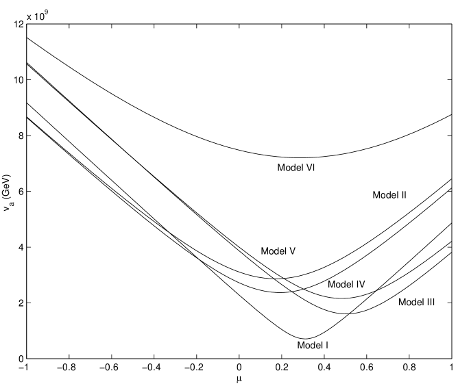
FIG. 1.: The lower bound on the axion decay constant $v_{a}$ for the axion models described in the text, plotted as a function of $\mu=\frac{v_{2}^{2}-v_{1}^{2}}{v_{EW}^{2}}$.