On the Determination of Small $x$ Shadowing Corrections at HERA

Abstract

The recent $F_{2}$ data can be described using the DGLAP evolution equations with an appropriate choice of input distributions and the choice of the starting scale for the $Q^{2}$ evolution. We demonstrate in this paper that we cannot conclude that there are no significant shadowing corrections at HERA kinematic region using $F_{2}$ data only. In this paper we calculate the shadowing corrections to the longitudinal structure function $F_{L}(x,Q^{2})$ and to the charm component of the proton structure function $F_{2}^{c}(x,Q^{2})$ at the HERA kinematic region using an eikonal approach. We demonstrate that the shadowing corrections to these observables are very large and that the charm production is strongly modified at small-$x$. Our results agree with the recent few H1 data.

I Introduction

The parton high density regime in deep inelastic scattering is one of the frontiers in perturbative QCD (pQCD). This corresponds to the small Bjorken $x$ region and represents the challenge of studying the interface between perturbative and non-perturbative QCD, with the peculiar feature that this transition is taken in a kinematical region where the strong coupling constant $\alpha_{s}$ is small. The transition between the perturbative regime and the non-perturbative regime may provide an understanding of the soft interactions in the language of QCD and establish whether the Regge model can be justified from QCD principles. From the experimental side, data from electron-proton collider HERA at DESY ($\sqrt{s}=300\,GeV$), provide new insights into the structure of the proton. The high energy allows to probe the proton in hitherto unexplored kinematical regions. The collider HERA allows the measure of structure functions $F_{2},\,F_{2}^{c}$, $F_{L}$ and the cross sections of vector meson production and diffractive processes for Bjorken $x$ values down to $10^{-4}$.

In the region of moderate $x$ ($x\geq 10^{-2}$) the well-established methods of operator expansion and renormalization group equations have been applied successfully. The DGLAP equations [1], which are based upon the sum of QCD ladder diagrams, are the evolution equations in this kinematical region. However, in the small $x$ region, the density of gluons and quarks becomes very high and a new dynamical effect is expected to stop the further growth of the structure functions. In this kinematical region we are dealing with a system of partons which are still at small distances, where $\alpha_{s}$ is still small, but the density of partons becomes so large that the usual methods of pQCD cannot be applied [2]. About seventeen years ago, Gribov et al. [3] have performed a detailed study of this region. They argued that the physical processes of interaction and recombination of partons become important in the parton cascade at a large value of the parton density, and that these shadowing corrections could be expressed in a new evolution equation - the GLR equation. This equation considers the leading non-ladder contributions: the multi-ladder diagrams, denoted as fan diagrams. The main characteristics of this equation are: it predicts a saturation of the gluon distribution at very small $x$; it predicts a critical line, separating the perturbative regime from the saturation regime; it is only valid in the border of this critical line. Therefore, the GLR equation predicts the limit of its validity. In the last decade, the solution [4, 5, 6] and possible generalizations [7, 8] of the GLR equation have been studied in great detail. Recently, an eikonal approach to the shadowing corrections was proposed in the literature [9, 10, 11]. The starting point of these papers is the proof of the Glauber formula in QCD [12], which considers only the interaction of the fastest partons with the target. As in QCD we rather expect that all partons should interact with the target, a more general approach was proposed in [9]. This approach was applied to the nuclear case in [9] and to the nucleon case in [10, 11]. Some of the main characteristics of this approach are its validity in a large kinematic region and that it provides a limit case of the GLR equation. In this paper the shadowing corrections will be estimated using the eikonal approach. In the next section we discuss this approach in more detail, pointing first our motivation.

One of the most striking discoveries at HERA is the steep rise of the proton structure function $F_{2}(x,Q^{2})$ with decreasing Bjorken $x$ [13]. The behaviour of the structure function at small $x$ is driven by the gluon through the process $g\rightarrow q\overline{q}$. Therefore the gluon distribution is the observable that governs the physics of high energy processes in QCD. HERA shows that the deep inelastic structure function $F_{2}(x,Q^{2})$ has a steep behaviour in the small-$x$ region $(10^{-2}>x>10^{-5})$, even for very small virtualities $(Q^{2}\approx 1\,GeV^{2})$. Indeed, considering $F_{2}\propto x^{-\lambda}$ at low $x$, the HERA data are consistent with a $\lambda$ that varies from 0.15 at $Q^{2}=0.85\,GeV^{2}$ to 0.4 at $Q^{2}=20\,GeV^{2}$. This steep behaviour is well described in the framework of the DGLAP evolution equations with an appropriate choice of input distributions and the choice of the starting scale for the $Q^{2}$ evolution, by all groups doing global fits of the data [14, 15, 16]. No other ingredient is needed to describe the experimental data. Using this result is it possible to conclude that there will be no significant shadowing contributions at HERA small-$x$ regime? Here, we address this question. Clearly, the answer of this question is connected with the demonstration that the corrections due to shadowing corrections (SC) are negligible at least at HERA kinematic region. If it is not so the DGLAP approach is not better or worse than any other evolution mechanism developed to describe the experimental data.

The SC for the $F_{2}(x,Q^{2})$ proton structure function and $xG(x,Q^{2})$ gluon distribution were computed considering the eikonal approach in refs. [10, 11] . In those works, the authors estimate the value of the SC which turn out to be essential in the gluon distribution but rather small in $F_{2}$. Consequently, the $F_{2}$ data cannot determine if there is a new dynamical effect at HERA. Therefore, to obtain a more precise evidence of SC at HERA kinematic region, we must consider other observables directly dependent on the behaviour of the gluon distribution, and consequently, more sensitive to SC. Some of these observables are $F_{L}$, $F_{2}^{c}$, $J/\Psi$ production, diffractive leptoproduction of vector mesons and open charm production. In this paper we consider the observables $F_{L}$ and $F_{2}^{c}$. The dominant charm production mechanism is the boson-gluon fusion. Therefore, the charm component $F_{2}^{c}$ of the structure function is a sensitive probe of the gluon distribution at small $x$. Furthermore, the violation of the Callan-Gross relation ($F_{L}=F_{2}-2xF_{1}=0$) occurs when the quarks acquire transverse momenta from QCD radiation. Consequently, also the longitudinal structure function is a sensitive probe of the gluon distribution at small $x$. In this work we estimate the SC in $F_{L}$ and $F_{2}^{c}$ in the approach proposed in [10]. We calculate these observables using the Altarelli-Martinelli equation [17] and the boson-gluon fusion cross section [14], respectively. The gluon distribution and the $F_{2}$ structure function necessary to these equations are calculated considering the eikonal approach. Actually, there are few data in these observables, but more measurements, with better statistics, will be available in the next years. Therefore it is very important the analysis of the behaviour of these observables considering SC.

This paper is organized as follows. In Section II the eikonal approach and the shadowing corrections for the $F_{2}(x,Q^{2})$ and $xG(x,Q^{2})$ are briefly presented. In Section III we obtain the formulae for the calculation of the $F_{L}$ and $F_{2}^{c}$ and we apply our results to HERA data. Moreover, we compare our results with the predictions of DGLAP dynamics. Finally, in Section IV, we present our conclusions.

II The Eikonal Approach in pQCD

The space-time picture of the Eikonal approach in the target rest frame can be viewed as the decay of the virtual gluon at high energy (small $x$) into a gluon-gluon pair long before the interaction with the target. The $gg$ pair subsequently interacts with the target. In the small $x$ region, where $x<<\frac{1}{2mR}$ ($R$ is the size of the target), the $gg$ pair crosses the target with fixed transverse distance $r_{t}$ between the gluons.

The cross section of the absorption of a gluon $g^{*}$ with virtuality $Q^{2}$ can be written as

$$\sigma^{g^{*}+nucleon}(x,Q^{2})=\int_{0}^{1}dz\int\frac{d^{2}r_{t}}{\pi}\int\frac{d^{2}b_{t}}{\pi}|\Psi_{t}^{g^{*}}(Q^{2},r_{t},x,z)|^{2}\sigma^{gg+nucleon}(z,r_{t}^{2})\,\,,$$ (1)

where $z$ is the fraction of energy carried by the gluon, $b_{t}$ is the impact parameter and $\Psi_{t}^{g^{*}}$ is the wave function of the transverse polarized gluon in the virtual probe. Furthermore, $\sigma^{gg+nucleon}(z,r_{t}^{2})$ is the cross section of the interaction of the $gg$ pair with the nucleon. In the leading log$(1/x)$ approximation we can neglect the change of $z$ during the interaction and describe the cross section $\sigma^{gg+nucleon}(z,r_{t}^{2})$ as a function of the variable $x$.

Using the unitarity in the $s$-channel, the cross section $\sigma^{gg+nucleon}(z,r_{t}^{2})=\sigma(x,r^{2}_{t})$ can be written in the form

$$\sigma(x,r^{2}_{t})=2\int d^{2}b_{t}\,(1-e^{-\frac{1}{2}\Omega(x,r_{t},b_{t})})\,\,,$$ (2)

where $\Omega$ is an arbitrary real function, which can be specified only in a more detailed theory or approach than the unitarity constraint. One of such specified model is the Eikonal model.

The Eikonal model assumes that $\Omega$ is small $(\Omega<<1)$ and its $b_{t}$ dependence can be factorized as $\Omega=\overline{\Omega}S(b_{t})$, with the normalization $\int d^{2}b_{t}\,S(b_{t})=1$. The factorization was proven for the DGLAP evolution equations [3] and, therefore, all our further calculations will be valid for the DGLAP evolution equations in the region of small $x$ or, in other words, in the double log approximation (DLA) of perturbative QCD (pQCD). The Eikonal approach is the assumption that $\Omega=\overline{\Omega}S(b_{t})$ in the whole kinematical region.

In [18] the authors demonstrate that $\overline{\Omega}$ is given by

$$\overline{\Omega}=\sigma_{N}^{gg}=\frac{3\alpha_{s}(\frac{4}{r_{t}^{2}})}{4}\,\pi^{2}\,r_{t}^{2}\,xG(x,\frac{4}{r_{t}^{2}})\,\,,$$ (3)

where $xG(x,Q^{2})$ is the gluon distribution. Therefore the behaviour of the cross section (2) in the small-$x$ region is determinated by the behaviour of the gluon distribution in this region.

Considering the $s$-channel unitarity and the eikonal model, equation (1) can be written as

$$\sigma^{g^{*}+nucleon}(x,Q^{2})=\int_{0}^{1}dz\int\frac{d^{2}r_{t}}{\pi}\int\frac{d^{2}b_{t}}{\pi}|\Psi_{t}^{g^{*}}(Q^{2},r_{t},x,z)|^{2}\,(1-e^{-\frac{1}{2}\overline{\Omega}S(b_{t})})\,\,,$$ (4)

Using the relation $\sigma^{g^{*}+nucleon}(x,Q^{2})=\frac{4\pi^{2}\alpha_{s}}{Q^{2}}xG(x,Q^{2})$ and the expression of the wave $\Psi^{g^{*}}$ calculated in [9], the Glauber-Mueller formula for the gluon distribution is obtained as

$$xG(x,Q^{2})=\frac{4}{\pi^{2}}\int_{x}^{1}\frac{dx^{\prime}}{x^{\prime}}\int_{\frac{4}{Q^{2}}}^{\infty}\frac{d^{2}r_{t}}{\pi r_{t}^{4}}\int_{0}^{\infty}\frac{d^{2}b_{t}}{\pi}\,2\,[1-e^{-\frac{1}{2}\sigma_{N}^{gg}(x^{\prime},\frac{r_{t}^{2}}{4})S(b_{t})}]\,\,.$$ (5)

The use of the Gaussian parameterization for the nucleon profile function $S(b_{t})=\frac{1}{\pi R^{2}}e^{-\frac{b^{2}}{R^{2}}}$ simplifies the calculations. Consequently, doing the integral over $b_{t}$, the master equation is obtained

$$xG(x,Q^{2})=\frac{2R^{2}}{\pi^{2}}\int_{x}^{1}\frac{dx^{\prime}}{x^{\prime}}\int_{\frac{1}{Q^{2}}}^{\frac{1}{Q_{0}^{2}}}\frac{d^{2}r_{t}}{\pi r_{t}^{4}}\{C+ln(\kappa_{G}(x^{\prime},r_{t}^{2}))+E_{1}(\kappa_{G}(x^{\prime},r_{t}^{2}))\}\,\,,$$ (6)

where $C$ is the Euler constant, $E_{1}$ is the exponential function, and the function $\kappa_{G}(x,r_{t}^{2})=\frac{3\alpha_{s}}{2R_{A}^{2}}\,\pi\,r_{t}^{2}\,xG(x,\frac{1}{r_{t}^{2}})$. If equation (6) is expanded for small $\kappa_{G}$, the first term (Born term) will correspond to the usual DGLAP equation in the small $x$ region, while the other terms will take into account the shadowing corrections.

The master formula (6) is correct in the double logarithmic approximation (DLA) [10]. As shown in [10] the DLA does not work quite well in the accessible kinematic region ($Q^{2}>1\,GeV^{2}$ and $x>10^{-4}$). Consequently, a more realistic approach must be considered to calculate the gluon distribution $xG$. In [10] the subtraction of the Born term of (6) and addition of the GRV parameterization was proposed. This procedure gives

$$xG(x,Q^{2}) = xG^{master}[\mbox{eq. (\ref{master})}]+xG^{GRV}(x,Q^{2})$$ (7)

$$- \frac{\alpha_{s}N_{c}}{\pi}\int_{x}^{1}\int_{Q_{0}^{2}}^{Q^{2}}\frac{dx^{\prime}}{x^{\prime}}\frac{dQ^{\prime 2}}{Q^{\prime 2}}\,x^{\prime}G^{GRV}(x^{\prime},Q^{\prime 2})\,\,.$$ (8)

The above equation includes also $xG^{GRV}(x,Q_{0}^{2})$ as the initial condition for the gluon distribution and gives $xG^{GRV}(x,Q^{2})$ as the first term of the expansion with respect to $\kappa_{G}$. Therefore, this equation is an attempt to include the full expression for the anomalous dimension for the scattering off each nucleon, while the use of the DLA takes into account all SC. In [9] this procedure was applied to obtain the shadowing corrections to the nuclear gluon distribution and in [10] to the nucleon gluon distribution.

The equation (5) is not a non-linear equation type the GLR equation [3]; it is the analogue of the Glauber formula, which provides the possibility to calculate the SC using the solution of the DGLAP evolution equation. In this paper, as shown in eq. (8), we use the GRV parameterization as a solution of the DGLAP evolution equation. It describes all available experimental data quite well [13]. It should be also stressed here that we disregard how much of SC has been taken into account in this parameterization in the form of the initials distributions.

A similar approach can be used to obtain the SC for the deep inelastic structure function $F_{2}(x,Q^{2})$. This was made in the references [10, 18]. The main result of these references is that the structure function $F_{2}$ can be written, in the eikonal approach, as

$$F_{2}(x,Q^{2})=\frac{N_{c}}{6\pi^{3}}\sum_{u,d,s}\epsilon_{q}^{2}\int_{\frac{1}{Q^{2}}}^{\infty}\frac{d^{2}r_{t}}{r_{t}^{4}}\int d^{2}b_{t}\{1-e^{-\frac{1}{2}\Omega_{q\overline{q}}(x,r_{t},b_{t})}\}\,\,,$$ (9)

where $\Omega_{q\overline{q}}=\frac{4}{9}\overline{\Omega}S(b_{t})$ (see eq. (3)).

Following the same steps used in the case of the gluon distribution, the proton structure function can be written as

$$F_{2}(x,Q^{2})=\frac{2R^{2}}{3\pi^{2}}\sum_{u,d,s}\epsilon_{q}^{2}\int_{\frac{1}{Q^{2}}}^{\frac{1}{Q_{0}^{2}}}\frac{d^{2}r_{t}}{\pi r_{t}^{4}}\{C+ln(\kappa_{q}(x,r_{t}^{2}))+E_{1}(\kappa_{q}(x,r_{t}^{2}))\}\,\,,$$ (10)

where $\kappa_{q}=\frac{4}{9}\kappa_{G}$. Similarly as made in the case of the gluon distribution, to obtain a more realistic approach the Born term must be subtracted and the GRV parameterization must be summed. Therefore the proton structure function is given by

$$F_{2}(x,Q^{2})=F_{2}(x,Q^{2})[\mbox{eq. (\ref{diseik2})}]-F_{2}(x,Q^{2})[\mbox{Born}]+F_{2}(x,Q^{2})[\mbox{GRV}]\,\,,$$ (11)

where $F_{2}(x,Q^{2})[\mbox{Born}]$ is the first term in the expansion in $\kappa_{q}$ of the equation (10), and

$$F_{2}(x,Q^{2})[\mbox{GRV}]=\sum_{u,d,s}\epsilon_{q}^{2}\,[xq(x,Q^{2})+x\overline{q}(x,Q^{2})]+F_{2}^{c}(x,Q^{2})$$ (12)

is calculated using the GRV parameterization.

In [10] the shadowing corrections for the $F_{2}(x,Q^{2})$ proton structure function and $xG(x,Q^{2})$ gluon distribution were computed considering the eikonal approach, and the SC which turn out to be essential in the gluon distribution are rather small in $F_{2}$.

The result above is demonstrated in figure 1, where we present the ratios

$$R_{1}=\frac{xG^{GM}(x,Q^{2})}{xG^{GRV}(x,Q^{2})}$$ (13)

and

$$R_{2}=\frac{F_{2}^{GM}(x,Q^{2})}{F_{2}^{GRV}(x,Q^{2})}\,\,,$$ (14)

as a function of variable $ln(\frac{1}{x})$ for different values of $Q^{2}$. In this case $GM$ represents that the function ($F_{2}$ or $xG$) was obtained using the eikonal approach, and $GRV$ represents that the function was obtained using the GRV parameterizations [14]. We can see that in HERA kinematical region $(3\leq\,ln\,\frac{1}{x}\,\leq 12)$ the behaviour of the gluon distribution is strongly modified by shadowing corrections. In [10] the authors demonstrated that the $F_{2}$ data can be described considering shadowing corrections, i.e. the $F_{2}$ data cannot determinate if there is a new dynamical effect at HERA. Consequently, observables directly dependent on the behaviour of the gluon distribution must be considered to discriminate the SC. From results obtained in [10] we conclude that the eikonal model provides a good description of the SC and can be taken as a correct approximation in the approach to the nucleon case for HERA kinematical region. In the next section we estimate the shadowing corrections to observables directly dependent on the behaviour of the gluon distribution.

In this paper we estimate the shadowing corrections using an eikonal approach proposed in [10]. The eikonal approach gives sufficiently reliable results for the HERA kinematic region, however, it is not the most efficient way to calculate the shadowing corrections. In [10], a generalized equation which takes into account the interaction of all partons in a parton cascade with the target was proposed. The main properties of generalized equation are: (i) the iterations of this equation coincide with the iteration of the Glauber-Mueller formula; (ii) its solution matches the solution of the DGLAP evolution equation in the double-logarithmic-approximation (DLA) limit of pQCD; (iii) it has the GLR equation as a limit, and (iv) contains the Glauber-Mueller formula. Therefore, the generalized equation is valid in a large kinematic region. In this paper we have used the Glauber-Mueller formula, since that in the HERA kinematic region the solutions of the generalized equation and of Glauber-Mueller formula are approximately identical [10]. However, a more accurate approach, to a larger kinematic region than the HERA one, should consider as an input the solution of the generalized equation, in the future [19].

III $F_{L}$ and $F_{2}^{c}$

Our goal in this section is the determination of small-$x$ shadowing corrections at $F_{L}$ and $F_{2}^{c}$ using the approach proposed in [10]. These observables are directly dependent on the behaviour of the gluon distribution, and consequently, more sensitive to SC.

Recently, the SC to the $F_{2}$ slope was estimated [20]. This observable is also directly dependent on the behaviour of the gluon distribution [21]. It was shown that the contribution of SC is large in the $F_{2}$ slope and that the experimental data can be described incorporating the SC. This result is a strong motivation to estimate the SC at $F_{L}$ and $F_{2}^{c}$.

A The longitudinal structure function

The longitudinal structure function in deep inelastic scattering is one of the observables from which the gluon distribution can be unfolded. Its experimental determination is difficult since it usually requires cross sections measurements at different values of center of mass energy, implying a change of beam energies. A direct change of the beam energies at HERA has been widely discussed [22]. An alternative possibility is to apply the radiation of a hard photon by the incoming electron. Such hard radiation results into an effective reduction of the center of mass energy. Several studies on the use of such events to measure $F_{L}$ have been carried out [23]. With these measurements, which in principle could be performed in the near future, it may be possible to explore the structure of $F_{L}(x,Q^{2})$ in the low $x$ range.

Current measurements of $R(x,Q^{2})=F_{L}/(F_{2}-F_{L})$ have been made by various fixed target lepton-hadron scattering experiments at higher $x$ values [24]. At low $x$, the measurements of this observable are very scarce. Recently, the H1 Collaboration has published the first $F_{L}$ data at small $x$. To obtain the data, the structure function $F_{2}$ was parameterized taken only data for $y<0.35$, where the contribution of $F_{L}$ is small. The quantity $y=\frac{Q^{2}}{sx}$ describes in the rest frame of the proton, the energy transfer from the incoming to the outgoing electron. This parameterization was evolved in $Q^{2}$ according to the DGLAP evolution equations. This provides predictions for the structure function $F_{2}$ in the high $y$ region which allowed, by subtraction of the contribution of $F_{2}$ to the cross section, the determination of the longitudinal structure function. Therefore, in order to constrain the value of $F_{L}$ in low $x$ regime explored by HERA, the H1 Collaboration extracted $F_{L}$ assuming that the DGLAP evolution holds. Our point of view agrees with Thorne’s statement [26], pointing that the assumption of the correctness of the DGLAP evolution equations at small $x$ implies that $F_{L}$ is already isolated. Therefore, our comparisons with these data must be considered as an estimate of the SC compared with the results of the standard evolution equations.

One can write the longitudinal structure function $F_{L}$ in terms of the cross section for the absorption of longitudinally polarized photons as

$$F_{L}(x,Q^{2})=\frac{Q^{2}(1-x)}{4\pi^{2}\alpha_{em}}\,\sigma_{L}(x,Q^{2})\approx\frac{Q^{2}}{4\pi^{2}\alpha_{em}}\,\sigma_{L}(x,Q^{2})$$ (15)

at small $x$. Longitudinal photons have zero helicity and can exist only virtually. In the Quark-Parton Model (QPM), helicity conservation of the electromagnetic vertex yields the Callan-Gross relation, $F_{L}=0$, for scattering on quarks with spin $1/2$. This does not hold when the quarks acquire transverse momenta from QCD radiation. Instead, QCD yields the Altarelli-Martinelli equation[17]

$$F_{L}(x,Q^{2})=\frac{\alpha_{s}(Q^{2})}{2\pi}\,x^{2}\,\int_{x}^{1}\frac{dy}{y^{3}}[\frac{8}{3}\,F_{2}(y,Q^{2})+4\,\sum_{q}e_{q}^{2}(1-\frac{x}{y})yg(y,Q^{2})]\,\,,$$ (16)

expliciting the dependence of $F_{L}$ on the strong constant coupling and the gluon density. At small $x$ the second term with the gluon distribution is the dominant one. Consequently, the expression (16) can be approximated reasonably by $F_{L}(x,Q^{2})\approx 0.3\,\frac{4\alpha_{s}}{3\pi}xg(2.5x,Q^{2})$ [27]. This equation demonstrates the close relation between the longitudinal structure function and the gluon distribution. Therefore, we expect that the longitudinal structure function to be sensitive to the shadowing corrections at HERA kinematic region. In this paper we calculate $F_{L}$ using the Altarelli-Martinelli equation (16).

Considering the expressions (8), (11) and (16) we can estimate the SC for the $F_{L}$ structure function. In figure 2 we present the ratio

$$R_{L}=\frac{F_{L}^{GM}(x,Q^{2})}{F_{L}^{GRV}(x,Q^{2})}\,\,,$$ (17)

where $F_{L}^{GM}(x,Q^{2})$ indicates that the longitudinal structure function was obtained using the gluon distribution solution of the Glauber-Mueller formula, eq. (5), and $F_{L}^{GRV}(x,Q^{2})$ indicates that $F_{L}$ was obtained using the GRV parameterization. We can see that the behaviour of $F_{L}$ is strongly modified by shadowing corrections. The suppression increases with $ln(\frac{1}{x})$ and is much bigger than for the $F_{2}$ case. In the region of HERA data, $3\leq\,ln(\frac{1}{x})\leq\,12$, the shadowing corrections are not bigger than $44\%$ ($ln(\frac{1}{x})\approx 12$). The SC are as big as $70\%$ only at very small value of $x$ ($ln(\frac{1}{x})\approx 15$), where we have no experimental data.

In figure 3 we present the behaviour of the $F_{L}$ structure function with (dashed curve) and without shadowing (solid curve) as a function of $ln(\frac{1}{x})$ for different virtualities. We compare our results with the scarce H1 data [25]. We can see that both curves agree with the data, however the experimental error are still very large. In figure 4 we present our results for $F_{L}$ and compare with all H1 data. From the above results we can conclude that the eikonal model gives a good description of the longitudinal structure function and describes the experimental data. However, new data, with better statistics, could verify the shadowing corrections at HERA kinematic region.

Our conclusion of this section is that the longitudinal structure function $F_{L}$ is a good observable to isolate the shadowing corrections at HERA. Consequently, we must stress the importance of measuring directly $F_{L}$ at HERA as a probe of the dynamics of small $x$ physics. We hope this result could also motivate the acquisition of new data in the next years.

B The charm component $F_{2}^{c}$ of the structure function

The problem of how to treat heavy quark contributions in the deep inelastic structure functions has been widely discussed, see for example [28]. It has been brought into focus recently by the very precise $F_{2}(x,Q^{2})$ data from HERA [13]. Both the H1 and ZEUS collaborations have measured the charm component $F_{2}^{c}$ of the structure function at small $x$ and have found it to be a large (approximately $25\%$) fraction of the total. This is in sharp contrast to what is found at large $x$, where typically $F_{2}^{c}/F_{2}\,\approx{\cal{O}}(10^{-2})$.

For the treatment of the charm component of the structure function there are basically two different prescriptions for the charm production in the literature. The first one is advocated in [29] where the charm quark is treated as a heavy quark and its contribution is given by fixed-order perturbation theory. This involves the computation of the boson-gluon fusion process. In the other approach [30] the charm is treated similarly to a massless quark and its contribution is described by a parton density in a hadron. Here our goal is to obtain the shadowing corrections to the charm structure function in the eikonal approach, without considering in detail the question of how to treat heavy quark contributions [28]. However, some comments are important. We consider the charm production via boson-gluon fusion, where the charm is treated as a heavy quark and not a parton. This scheme is usually called Fixed Flavour Number Scheme (FFNS). In this scheme, by definition, only light partons (e.g. $u$, $d$, $s$ and $g$) are included in the initial state for charm production: the number of parton flavours $n_{f}$ is kept at a fixed value regardless the energy scales involved. The boson-gluon fusion gives the correct description of $F_{2}^{c}$ for $Q^{2}<4m_{c}^{2}$ and should remain a reasonable approximation to $F_{2}^{c}$ for $Q^{2}\geq 4m_{c}^{2}$. However, the boson-gluon fusion model will inevitably break down at larger $Q^{2}$ values as the charm can no longer be treated as a non-partonic heavy object, and begins to evolve more like the lighter components of the quark sea. Therefore, our estimates in this scheme should be considered with caution in the region of large $Q^{2}$.

A $c\overline{c}$ pair can be created by boson-gluon fusion when the squared invariant mass of the hadronic final state $W^{2}\geq 4m_{c}^{2}$. Since $W^{2}=\frac{Q^{2}(1-x)}{x}+M_{N}^{2}$, where $M_{N}$ is the nucleon mass, the charm production can occur well below the $Q^{2}$ threshold, $Q^{2}\approx 4m_{c}^{2}$, at small $x$. The charm contribution to the proton structure function, in leading order (LO), is given by [14]

$$\frac{1}{x}F_{2}^{c}(x,Q^{2},m_{c}^{2})=2e_{c}^{2}\frac{\alpha_{s}(\mu^{\prime 2})}{2\pi}\int_{ax}^{1}\frac{dy}{y}\,C_{g,2}^{c}(\frac{x}{y},\frac{m_{c}^{2}}{Q^{2}})\,g(y,\mu^{\prime 2})\,\,,$$ (18)

where $a=1+\frac{4m_{c}^{2}}{Q^{2}}$ and the factorization scale $\mu^{\prime}$ is assumed $\mu^{\prime 2}=4m_{c}^{2}$. $C_{g,2}^{c}$ is the coefficient function given by

$$C_{g,2}^{c}(z,\frac{m_{c}^{2}}{Q^{2}}) = \frac{1}{2}\{[z^{2}+(1-z)^{2}+z(1-3z)\frac{4m_{c}^{2}}{Q^{2}}-z^{2}\frac{8m_{c}^{4}}{Q^{4}}]ln\frac{1+\beta}{1-\beta}$$ (19)

$$+ \beta[-1+8z(1-z)-z(1-z)\frac{4m_{c}^{2}}{Q^{2}}]\}\,\,,$$ (20)

where $\beta=1-\frac{4m_{c}^{2}z}{Q^{2}(1-z)}$ is the velocity of one of the charm quarks in the boson-gluon center-of-mass frame. Therefore, in leading order, ${\cal{O}}(\alpha_{s})$, $F_{2}^{c}$ is directly sensitive only to the gluon density via the well-known Bethe-Heitler process $\gamma^{*}g\rightarrow c\overline{c}$. The dominant uncertainty in the QCD calculations arises from the uncertainty in the charm quark mass. In this paper we assume $m_{c}=1.5\,GeV$.

Considering the expressions (8) and (18) we can estimate the shadowing corrections for the $F_{2}^{c}$ structure function. In figure 5 we present the ratio

$$R_{2}^{c}=\frac{F_{2}^{c\,GM}(x,Q^{2})}{F_{2}^{c\,GRV}(x,Q^{2})}\,\,.$$ (21)

We can see that the behaviour of the $F_{2}^{c}$ is strongly modified by the SC. The suppression due to shadowing corrections increases with $ln(\frac{1}{x})$ and is much bigger than for the $F_{2}$ case. In the region of HERA data, $3\leq\,ln(\frac{1}{x})\leq\,12$, the SC are not bigger than $40\%$ ($ln(\frac{1}{x})\approx 12$). The SC are bigger than $62\%$ only at very small value of $x$ ($ln(\frac{1}{x})\approx 15$), where we have no experimental data.

In figure 6 we present the behaviour of the $F_{2}^{c}$ structure function with (dashed curve) and without shadowing (solid curve) for different virtualities. We compare our results with the H1 data [31]. Our predictions agree with the recent H1 data. When compared with the GRV parameterization the shadowing corrections to $F_{2}^{c}$ present a suppression which increases with $ln(\frac{1}{x})$. Therefore, new data, with better statistics, could isolate the shadowing corrections at HERA kinematic region.

As the shadowing corrections are distinct for the observables $F_{2}$ and $F_{2}^{c}$ we can estimate the modifications in the charm contribution to the $F_{2}$ at small $x$ by SC. In figure 7 we present our results for the ratio

$$R_{F}=\frac{F_{2}^{c}(x,Q^{2})}{F_{2}(x,Q^{2})}\,\,.$$ (22)

We can see that the behaviour of this ratio is strongly modified by the shadowing corrections. Therefore, we expect that the charm contribution do not increase at small values of $x$ when compared with the predictions obtained using the usual parameterizations. Furthermore, we expect a strong modification in the charm production at small $x$. It is one of the main conclusions of this paper. This strong modification in the charm production shall occur in other associated observables, for instance in $J/\Psi$ production. The shadowing corrections to the diffractive leptoproduction of vector meson $J/\Psi$ was calculated in [32]. The authors obtained that the SC are large, but their results are affected by the uncertainty in the $J/\Psi$ wavefunction. Consequently, although the cross section of diffractive leptoproduction of $J/\Psi$ is proportional to the square of the gluon distribution, the accurate discrimination of SC in this process is still unlikely.

Our conclusion of this section is that the charm component $F_{2}^{c}$ is also a good observable to isolate the shadowing corrections. Therefore, new data, with better statistics will be very important in the determination of dynamics at HERA, and further applications.

IV Conclusions

The pQCD has furnished a remarkably successful framework to interpret a wide range of high energy lepton-lepton, lepton-hadron and hadron-hadron processes. Through global analysis of these processes, detailed information on the parton structure of hadrons, especially the nucleon, has been obtained. The existing global analysis have been performed using the standard DGLAP evolution equations. However, in the small $x$ region the DGLAP evolution equations are expected to breakdown, since new effects must occur in this kinematical region. One of these effects is the shadowing phenomenon.

The recent $F_{2}$ data are well described in the framework of the DGLAP evolution equations with an appropriate choice of input distributions and the choice of the starting scale for the $Q^{2}$ evolution. Although no other ingredient has been needed to describe the data, we cannot conclude that the shadowing corrections are negligible at HERA kinematic region only from the analysis of $F_{2}$ data. The proton structure function is inclusive on the behaviour of the gluon distribution. In this paper we estimate the shadowing corrections to $F_{L}$ and $F_{2}^{c}$. The behaviour of these observables is directly dependent on the behaviour of the gluon distribution and, therefore, strongly sensitive to the shadowing corrections. We shown that the SC to $F_{L}$ and $F_{2}^{c}$ are much bigger than for the $F_{2}$ case. Our results are in accord with the recent few data. New data with better statistics are strongly welcome.

One of the main conclusions of this paper is the strong modification of charm component of the structure function. As the SC are different in the observables $F_{2}$ and $F_{2}^{c}$ the charm contribution do not increase at small $x$ as predicted by the usual parameterizations.

In this paper we estimate the shadowing corrections using an eikonal approach proposed in [10]. The eikonal approach gives a sufficiently reliable result for the HERA kinematic region, however, a more accurate approach, to a larger kinematic region than the HERA kinematic region, should consider as an input the solution of the generalized equation proposed in [10]. In a future publication we will estimate the behaviour of some observables using the solution of the generalized equation.

The determination of the dynamics at small $x$ is fundamental to estimate the cross sections of the processes which will be studied in the future accelerators. We expect that this paper could motivate a more accurate determination of $F_{L}$ and $F_{2}^{c}$ in the next years, since the behaviour of these observables may explicitate the dynamics at small $x$ regime.

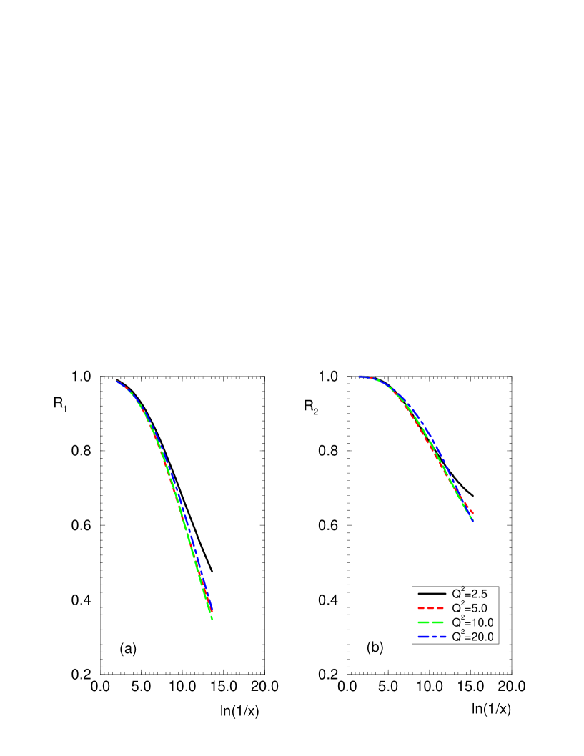
FIG. 1.: (a) The ratio $R_{1}=\frac{xG^{GM}}{xG^{GRV}}$ and (b) the ratio $R_{2}=\frac{F_{2}^{GM}}{F_{2}^{GRV}}$ as a function of the variable $ln(\frac{1}{x})$ for different virtualities.

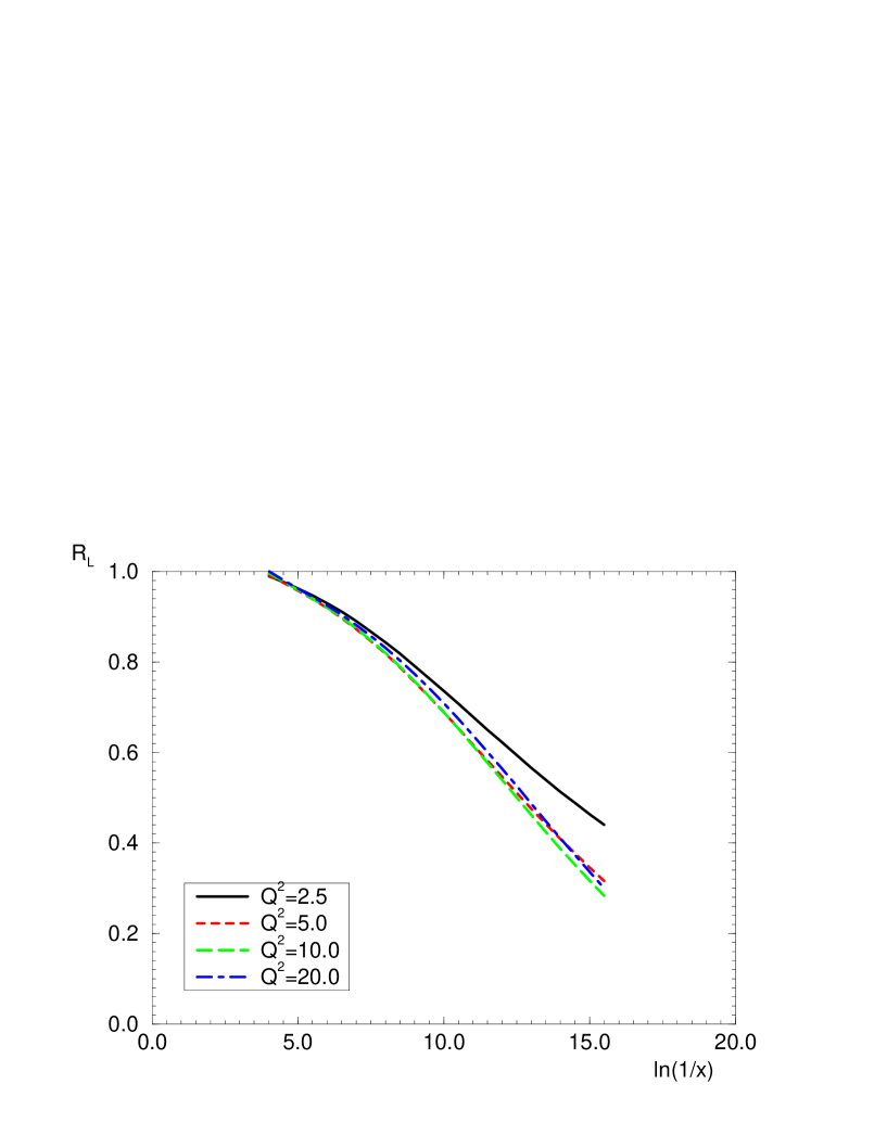
FIG. 2.: The ratio $R_{L}=\frac{F_{L}^{GM}}{F_{L}^{GRV}}$ as a function of the variable $ln(\frac{1}{x})$ for different virtualities.

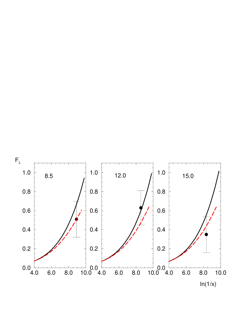
FIG. 3.: The longitudinal structure function $F_{L}$ for $Q^{2}=8.5,\,12,\,15\,GeV^{2}$. The solid curve represents that the $F_{L}$ was calculated using the GRV parameterization and the dashed curve that its was calculated using $xG$ and $F_{2}$ obtained in the eikonal model. Data from H1.

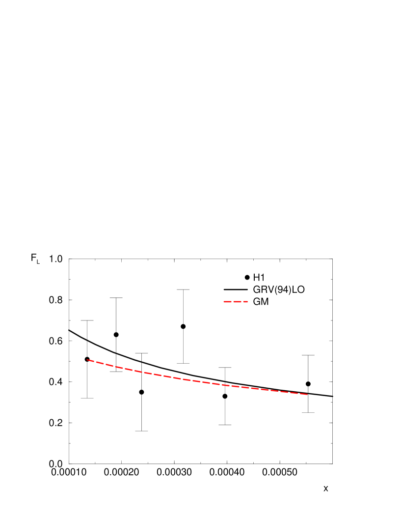
FIG. 4.: The longitudinal structure function $F_{L}$ for all H1 data.

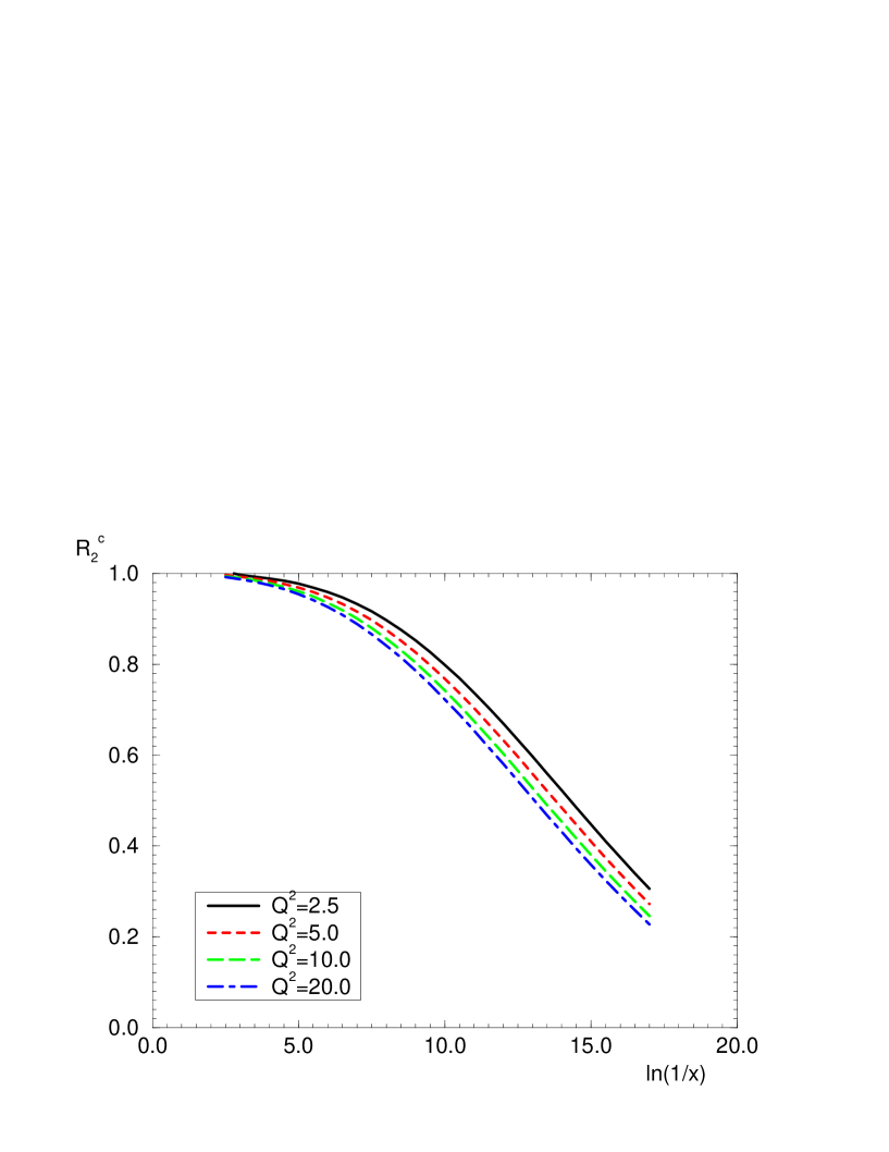
FIG. 5.: The ratio $R_{2}^{c}=\frac{F_{2}^{c\,GM}}{F_{2}^{\c{,}GRV}}$ as a function of the variable $ln(\frac{1}{x})$ for different virtualities.

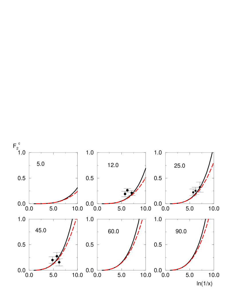
FIG. 6.: The charm component of the structure function for different values of $Q^{2}$. The solid curve represents $F_{2}^{c}$ calculated using the GRV parameterization and the dashed curve as calculated using $xG$ obtained from the eikonal model. Data are from H1.

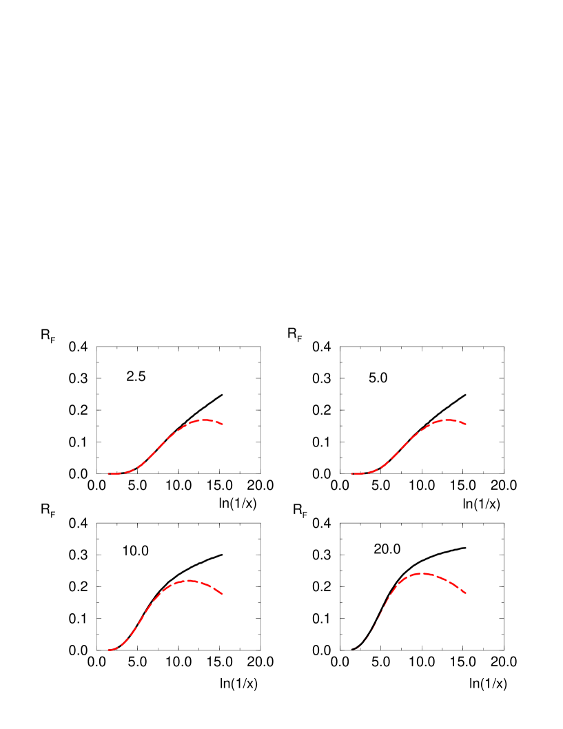
FIG. 7.: The ratio $R_{F}=\frac{F_{2}^{c}}{F_{2}}$ as a function of the variable $ln(\frac{1}{x})$ for different virtualities. The solid curve represents the predictions obtained using the GRV parameterization and the dashed curve the predictions obtained in the eikonal model.

REFERENCES

- [1] Yu. L. Dokshitzer. Sov. Phys. JETP 46, 641 (1977); G. Altarelli and G. Parisi. Nucl. Phys. B126, 298 (1977); V. N. Gribov and L.N. Lipatov. Sov. J. Nucl. Phys 28, 822 (1978).
- [2] E. Levin. III GWHEP. Proceedings of the 3rd Gleb Wataghin School on High Energy Phenomenology. Eds. J. Bellandi et al., 1994.
- [3] V. N. Gribov, E. M. Levin, M. G. Ryskin. Phys. Rep.100, 1 (1983).
- [4] J. Collins, J. Kwiecinski. Nucl. Phys. B335, 89 (1990).
- [5] J. Bartels, J. Blumlein, G. A. Schuler. Z. Phys. C50, 91 (1991).
- [6] J. Bartels, E. M. Levin. Nucl. Phys. B387, 617 (1992).
- [7] W. Zhu et al.. Phys. Lett B317, 200 (1993).
- [8] E. Laenen, E. M. Levin. Nucl. Phys. B451, 207 (1995).
- [9] A. L. Ayala, M. B. Gay Ducati and E. M. Levin. Nucl. Phys. B493, 305 (1997).
- [10] A. L. Ayala, M. B. Gay Ducati and E. M. Levin. Nucl. Phys. B511, 355 (1998).
- [11] A. L. Ayala, M. B. Gay Ducati and E. M. Levin. hep-ph/9710539.
- [12] A. H. Mueller. Nucl. Phys. B335, 115 (1990).
- [13] S. Aid et al.. Nucl. Phys. B470, 3 (1996).
- [14] M. Gluck, E. Reya and A. Vogt. Z. Phys. C67, 433 (1995).
- [15] A. D. Martin, R. G. Roberts, W. J. Stirling. Phys. Lett B387, 419 (1996).
- [16] H. L. Lai et al.. Phys. Rev. D55, 1280 (1997).
- [17] G. Altarelli, G. Martinelli. Phys. Lett B76, 89 (1978).
- [18] A. L. Ayala, M. B. Gay Ducati and E. M. Levin. Phys. Lett B388, 188 (1996).
- [19] E. M. Levin. hep-ph/9806434.
- [20] E. Gotsman, E. M. Levin, U. Maor. Phys. Lett B425, 369 (1998).
- [21] M. B. Gay Ducati, V. P. Gonçalves. Phys. Lett B390, 401 (1997).
- [22] Future Physics at HERA. Proceedings of the Workshop 1995/1996. Edited by G. Ingelman et al..
- [23] L. Favart et al.. Z. Phys. C72, 425 (1996).
- [24] M. Arneodo et al..Nucl. Phys. B483, 3 (1997).
- [25] C. Adloff et al.. Phys. Lett B393, 452 (1997).
- [26] R. S. Thorne. Phys. Lett B418, 371 (1998).
- [27] A. M. Cooper-Sarkar et al.. Z. Phys. C39, 281 (1988).
- [28] W. L. van Neerven. Acta Phys. Pol. B28, 2715 (1997).
- [29] M. Gluck, E. Reya, M. Stratmann.Nucl. Phys. B422, 37 (1994).
- [30] M. A. G. Aivazis et al.. Phys. Rev. D50, 3102 (1994).
- [31] C. Adloff et al.. Z. Phys. C72, 593 (1996).
- [32] E. Gotsman, E. M. Levin, U. Maor. Nucl. Phys. B464, 251 (1996).