TTP98–21
NYU–TH/98/04/02
MPI/PhT/98–032
FERMILAB–PUB–98/126–T
hep–ph/9807241
June 1998

Effective QCD Interactions of CP-odd Higgs Bosons at Three Loops

Abstract

In the virtual presence of a heavy quark $t$, the interactions of a CP-odd scalar boson $A$, with mass $M_{A}\ll 2M_{t}$, with gluons and light quarks can be described by an effective Lagrangian. We analytically derive the coefficient functions of the respective physical operators to three loops in quantum chromodynamics (QCD), adopting the modified minimal-subtraction ($\overline{\rm MS}$) scheme of dimensional regularization. Special attention is paid to the proper treatment of the $\gamma_{5}$ matrix and the Levi-Civita $\epsilon$ tensor in $D$ dimensions. In the case of the effective $ggA$ coupling, we find agreement with an all-order prediction based on a low-energy theorem in connection with the Adler-Bardeen non-renormalization theorem. This effective Lagrangian allows us to analytically evaluate the next-to-leading QCD correction to the $A\to gg$ partial decay width by considering massless diagrams. For $M_{A}=100$ GeV, the resulting correction factor reads $1+(221/12)\alpha_{s}^{(5)}(M_{A})/\pi+165.9\left(\alpha_{s}^{(5)}(M_{A})/\pi\right)^{2}\approx 1+0.68+0.23$. We compare this result with predictions based on various scale-optimization methods.

PACS numbers: 11.15.Me, 12.38.Bx, 13.30.Eg, 14.80.Cp

1 Introduction

Despite the tremendously successful consolidation of the standard model (SM) of elementary particle physics by experimental precision tests during the past few years, the structure of the Higgs sector has essentially remained unexplored, so that there is still plenty of room for extensions. A phenomenologically interesting extension of the SM Higgs sector that keeps the electroweak $\rho$ parameter [1] at unity in the Born approximation, is obtained by adding a second complex isospin-doublet scalar field with opposite hypercharge. This leads to the two-Higgs-doublet model (2HDM). After the three massless Goldstone bosons which emerge via the electroweak symmetry breaking are eaten up to become the longitudinal degrees of freedom of the $W^{\pm}$ and $Z$ bosons, there remain five physical Higgs scalars: the neutral CP-even $h$ and $H$ bosons, the neutral CP-odd $A$ boson, and the charged $H^{\pm}$-boson pair. The Higgs sector of the minimal supersymmetric extension of the SM (MSSM) consists of such a 2HDM. At tree level, the MSSM Higgs sector has two free parameters, which are usually taken to be the mass $M_{A}$ of the $A$ boson and the ratio $\tan\beta=v_{2}/v_{1}$ of the vacuum expectation values of the two Higgs doublets. For large values of $\tan\beta$, the top Yukawa couplings of the neutral Higgs bosons, $\Phi=h,H,A$, are suppressed compared to the bottom ones.

The search for Higgs bosons and the study of their properties are among the prime objectives of the Large Hadron Collider (LHC), a proton-proton colliding-beam facility with centre-of-mass energy $\sqrt{s}=14$ GeV, which is presently under construction at CERN. The dominant production mechanisms for the neutral Higgs bosons at the LHC will be gluon fusion, $gg\to\Phi$ [2], and $b\bar{b}\Phi$ associated production, $gg,q\bar{q}\to b\bar{b}\Phi$ [3], which is, however, only relevant for large $\tan\beta$. The loop-induced $gg\Phi$ couplings [4] are mainly mediated by virtual top quarks, unless $\tan\beta$ is very large, in which case the bottom-quark loops take over. The $ggh$ and $ggH$ couplings also receive contributions from squark loops, which are, however, insignificant for squark masses in excess of about 500 GeV [5]. In the case of the $ggA$ coupling, such contributions do not occur at one loop because the $A$ boson has no tree-level couplings to squarks. For small $\tan\beta$, the inclusive cross sections of $pp\to\Phi+X$ via gluon fusion are significantly increased, by typically 50–70% under LHC conditions, by including their leading QCD corrections, which involve two-loop contributions [6, 7]. Thus, the theoretical predictions for these observables cannot yet be considered to be well under control, and it is desirable to compute the next-to-leading QCD corrections at three loops, since there is no reason to expect them to be negligible. Recently, a first step in this direction has been taken by considering the resummation of soft-gluon radiation in $pp\to\Phi+X$, assuming $\tan\beta$ to be small [8].

Considering the enormous complexity of the exact expressions for the leading QCD corrections [7], it becomes apparent that, with presently available technology, the next-to-leading corrections are only tractable in limiting cases. For instance, in the large-$\tan\beta$ limit, where the $gg\Phi$ couplings are chiefly generated by bottom-quark loops, one can neglect the bottom-quark mass against the Higgs-boson mass, keeping the bottom Yukawa coupling finite. In this way, one resorts to massless QCD. On the other hand, if $\tan\beta$ is close to unity, which was assumed in Ref. [8], the top-quark loops play the dominant rôle, and simplifications occur if the mass hierarchy $M_{\Phi}\ll 2m_{t}$ is satisfied. Then, it is useful to construct an effective Lagrangian by integrating out the top quark. This effective Lagrangian is a linear combination of local composite operators of mass dimension four, which act in QCD with five massless quark flavours, while all dependence on $m_{t}$ is contained in their coefficient functions. Once the coefficient functions are known, it is sufficient to deal with massless Feynman diagrams. The effective Lagrangian describing the interactions of the SM Higgs boson $H$ with gluons and light quarks was elaborated at two loops in Ref. [9] and extended to three loops in Refs. [10, 11]. As an application, the ${\cal O}(\alpha_{s})$ [9] and ${\cal O}(\alpha_{s}^{2})$ [10] corrections to the $H\to gg$ partial decay width were calculated from this Lagrangian. These results can be readily adapted to the $h$ and $H$ bosons of the 2HDM with small $\tan\beta$ by accordingly adjusting the top Yukawa coupling, which appears as an overall factor.

In this paper, we extend the three-loop analysis of Refs. [10, 11] to include the $A$ boson of the 2HDM. As in Ref. [8], we work in the limit $\tan\beta\approx 1$, so that we may treat bottom as a massless quark flavour with vanishing Yukawa coupling, on the same footing as up, down, strange, and charm. Specifically, we construct a heavy-top-quark effective Lagrangian for the QCD interactions of the $A$ boson and derive from it an analytic result for the ${\cal O}(\alpha_{s}^{2})$ correction to the $A\to gg$ partial decay width appropriate for $M_{A}\ll 2m_{t}$. We recover the corresponding ${\cal O}(\alpha_{s})$ result originally found in Refs. [7, 12] and also discussed in Ref. [13]. The ${\cal O}(\alpha_{s})$ correction for arbitrary values of the $A$-boson and quark masses was presented in Ref. [7] as a two-fold parameter integral. Furthermore, it was shown that the leading high-$m_{t}$ term of this correction may also be obtained from massless five-flavour QCD endowed with a heavy-top-quark effective $ggA$ coupling [7, 14]. A central ingredient for this check was the observation that the effective $ggA$ coupling does not receive QCD corrections, at least at ${\cal O}(\alpha_{s})$. This fact was interpreted [7, 14] as being a consequence of the Adler-Bardeen theorem [15], which states that the anomaly of the axial-vector current [16] is not renormalized in QCD. This theorem is strictly proven to all orders in $\alpha_{s}$ for the abelian case [15], and strong arguments suggest that it also holds true for the nonabelian case [17]. In this paper, we verify by an explicit diagrammatic calculation that the ${\cal O}(\alpha_{s})$ and ${\cal O}(\alpha_{s}^{2})$ corrections to the coefficient function of the operator $G_{\mu\nu}^{a}\tilde{G}^{a\mu\nu}$, which generates the $A$-boson effective couplings to gluons vanish. We also present the leading-order coefficient function of the physical operator pertaining to the effective $q\bar{q}A$ interaction, where $q$ is a light quark. We thus provide the tools which are necessary to reduce the calculation of the next-to-leading QCD correction to the cross section of $pp\to A+X$ to a standard problem in massless five-flavour QCD.

In our analysis, we consistently neglect the Yukawa couplings of the light quarks to the $A$ boson. In other words, if all quark masses, except for $m_{t}$, are nullified, the hadronic decay width of the $A$ boson is entirely due to $A\to gg$ and the associated higher-order processes under consideration here. Through three loops, the contributing final states are $gggg$, $ggq\bar{q}$, $q\bar{q}q^{\prime}\bar{q}^{\prime}$, $ggg$, $gq\bar{q}$, $gg$, and $q\bar{q}$.

This paper is organized as follows. In Section 2, we establish the heavy-top-quark effective Lagrangian for the QCD interactions of the $A$ boson to three loops. In Section 3, we compute from this Lagrangian the ${\cal O}(\alpha_{s}^{2})$ correction to the partial width of the decay $A\to gg$ and compare it with predictions based on various scale-optimization methods. Section 4 contains a discussion of our results together with some remarks on the connection between the effective $ggA$ coupling, the axial-anomaly equation, and the low-energy theorem.

2 Effective Lagrangian

We start by setting up the theoretical framework for our analysis. As usual, we employ dimensional regularization in $D=4-2\varepsilon$ space-time dimensions and introduce a ’t Hooft mass, $\mu$, to keep the coupling constants dimensionless [18, 19]. We perform the renormalization according to the modified [20] minimal-subtraction [21] ($\overline{\rm MS}$) scheme. For the sake of generality, we take the QCD gauge group to be SU($N_{c}$), with $N_{c}$ arbitrary. The adjoint representation has dimension $N_{A}=N_{c}^{2}-1$. The colour factors corresponding to the Casimir operators of the fundamental and adjoint representations are $C_{F}=(N_{c}^{2}-1)/(2N_{c})$ and $C_{A}=N_{c}$, respectively. For the numerical evaluation, we set $N_{c}=3$. The trace normalization of the fundamental representation is $T=1/2$. As an idealized situation, we consider QCD with $n_{l}=n_{f}-1$ light quark flavours $q_{i}$ and one heavy flavour $t$, in the sense that $2m_{q_{i}}\ll M_{A}\ll 2m_{t}$. We wish to construct an effective $n_{l}$-flavour theory by integrating out the $t$ quark. We mark the quantities of the effective theory by a prime. Bare quantities carry the superscript “0”. As already mentioned in the Introduction, we consider a 2HDM with $\tan\beta=1$, so that the quark Yukawa couplings and masses are related by a flavour-independent proportionality factor.

The starting point of our consideration is the bare Yukawa Lagrangian for the interactions of the $A$ boson with the quarks in the full $n_{f}$-flavour theory,

$${\cal L}=-\frac{A^{0}}{v^{0}}\left(\sum_{i=1}^{n_{l}}m_{q_{i}}^{0}\bar{q}_{i}^{0}i\gamma_{5}q_{i}^{0}+m_{t}^{0}\bar{t}^{0}i\gamma_{5}t^{0}\right),$$ (1)

where $v=2^{-1/4}G_{F}^{-1/2}$, with $G_{F}$ being Fermi’s constant. Taking the limit $m_{t}^{0}\to\infty$ and keeping only leading terms, Eq. (1) may be written as a linear combination of pseudoscalar composite operators, $\tilde{O}_{i}^{\prime}$, with mass dimension four acting in the effective $n_{l}$-flavour theory. The resulting bare Lagrangian reads

$${\cal L}_{\rm eff}=-\frac{A^{0}}{v^{0}}\left(\tilde{C}_{1}^{0}\tilde{O}_{1}^{\prime}+\tilde{C}_{2}^{0}\tilde{O}_{2}^{\prime}+\ldots\right),$$ (2)

where

$$\tilde{O}_{1}^{\prime} = G_{\mu\nu}^{0\prime,a}\tilde{G}^{0\prime,a\mu\nu},$$

$$\tilde{O}_{2}^{\prime} = \partial_{\mu}J_{5}^{0\prime,\mu},\qquad J_{5}^{0\prime,\mu}=\sum_{i=1}^{n_{l}}\bar{q}_{i}^{0\prime}\gamma^{\mu}\gamma_{5}q_{i}^{0\prime},$$ (3)

$\tilde{C}_{i}^{0}$ are coefficient functions, which depend on the bare parameters of the full theory and carry all $m_{t}^{0}$ dependence, and the ellipsis stands for terms involving unphysical operators, which do not contribute to physical observables. Here, $G_{\mu\nu}^{a}=\partial_{\mu}G_{\nu}^{a}-\partial_{\nu}G_{\mu}^{a}+g_{s}f^{abc}G_{\mu}^{b}G_{\nu}^{c}$ is the colour-field-strength tensor and $\tilde{G}^{a\mu\nu}=\epsilon^{\mu\nu\rho\sigma}G_{\rho\sigma}^{a}$ is its dual; $G_{\mu}^{a}$ ($a=1,\ldots,N_{A}$) are the gluon fields, $g_{s}=\sqrt{4\pi\alpha_{s}}$ is the QCD gauge coupling, and $f^{abc}$ are the structure constants of the SU($N_{c}$) algebra. We do not display the colour indices of the quark fields. We mark the operators and coefficient functions with a tilde in order to avoid confusion with our previous notation for the scalar case [10, 11].

The Levi-Civita tensor $\epsilon^{\mu\nu\rho\sigma}$ is unavoidably a four-dimensional object and should be taken outside the R operation. Thus, we rewrite Eq. (3) as $\tilde{O}_{i}^{\prime}=\epsilon^{\mu\nu\rho\sigma}\tilde{O}_{i,\mu\nu\rho\sigma}^{\prime}$, where [19, 22, 23]

$$\tilde{O}_{1,\mu\nu\rho\sigma}^{\prime} = G_{[\mu\nu}^{0\prime,a}G_{\rho\sigma]}^{0\prime,a},$$

$$\tilde{O}_{2,\mu\nu\rho\sigma}^{\prime} = \frac{i}{3!}\sum_{i=1}^{n_{l}}\partial_{[\mu}\bar{q}_{i}^{0\prime}\gamma_{\nu}\gamma_{\rho}\gamma_{\sigma]}q_{i}^{0\prime}$$ (4)

are antisymmetrized in their four $D$-dimensional Lorentz indices. Furthermore, we substitute $\gamma_{5}=(i/4!)\epsilon^{\mu\nu\rho\sigma}\gamma_{[\mu}\gamma_{\nu}\gamma_{\rho}\gamma_{\sigma]}$ in Eq. (1). We then carry out the $D$-dimensional calculations with $\epsilon^{\mu\nu\rho\sigma}$ peeled off from the expressions. In the very end, after the renormalization is performed and the physical limit $\varepsilon\to 0$ is taken, we contract the expressions with $\epsilon^{\mu\nu\rho\sigma}$ to obtain the final results.

Prior to describing the actual calculation of $\tilde{C}_{i}^{0}$, let us discuss how Eq. (2) is renormalized. Since we are only interested in pure QCD corrections, we may substitute $A^{0}=A$ and $v^{0}=v$ in Eqs. (1) and (2). Denoting the renormalized counterparts of $\tilde{C}_{i}^{0}$ and $\tilde{O}_{i}^{\prime}$ by $\tilde{C}_{i}$ and $[\tilde{O}_{i}^{\prime}]$, the renormalized version of Eq. (2) takes the form

$${\cal L}_{\rm eff}=-2^{1/4}G_{F}^{1/2}A\left(\tilde{C}_{1}\left[\tilde{O}_{1}^{\prime}\right]+\tilde{C}_{2}\left[\tilde{O}_{2}^{\prime}\right]+\ldots\right),$$ (5)

where the ellipsis again represents unphysical terms. The divergence $\partial_{\mu}J_{5}^{0\prime,\mu}$ is renormalized multiplicatively in the same way as the colour-singlet axial-vector current $J_{5}^{0\prime,\mu}$ itself, while $G_{\mu\nu}^{0\prime,a}\tilde{G}^{0\prime,a\mu\nu}$ mixes under renormalization [23, 24]. Specifically, we have

$$\left[\tilde{O}_{1}^{\prime}\right] = Z_{11}^{\prime}\tilde{O}_{1}^{\prime}+Z_{12}^{\prime}\tilde{O}_{2}^{\prime},$$

$$\left[\tilde{O}_{2}^{\prime}\right] = Z_{22}^{\prime}\tilde{O}_{2}^{\prime},$$ (6)

where $Z_{22}^{\prime}=Z_{\rm MS}^{\rm s\prime}Z_{5}^{\rm s\prime}$ is the product of the standard ultraviolet (UV) renormalization constant $Z_{\rm MS}^{\rm s\prime}$ of the singlet axial current in the $\overline{\rm MS}$ scheme and the finite renormalization constant $Z_{5}^{\rm s\prime}$. The latter is introduced to restore the one-loop character of the operator relation of the axial anomaly,

$$\left[\tilde{O}_{2}^{\prime}\right]=\frac{\alpha_{s}^{(n_{l})}(\mu)}{\pi}\,\frac{Tn_{l}}{4}\left[\tilde{O}_{1}^{\prime}\right],$$ (7)

which is valid for Pauli-Villars regularization [23]. For the reader’s convenience, we list here the various renormalization constants to the order necessary for our purposes. They read [23]

$$Z_{11}^{\prime} = 1+\frac{\alpha_{s}^{(n_{l})}(\mu)}{\pi}\,\frac{1}{\varepsilon}\left(-\frac{11}{12}C_{A}+\frac{1}{3}Tn_{l}\right)+\left(\frac{\alpha_{s}^{(n_{l})}(\mu)}{\pi}\right)^{2}$$

$${}\times\left[\frac{1}{\varepsilon^{2}}\left(\frac{121}{144}C_{A}^{2}-\frac{11}{18}C_{A}Tn_{l}+\frac{1}{9}T^{2}n_{l}^{2}\right)+\frac{1}{\varepsilon}\left(-\frac{17}{48}C_{A}^{2}+\frac{1}{8}C_{F}Tn_{l}+\frac{5}{24}C_{A}Tn_{l}\right)\right],$$

$$Z_{12}^{\prime} = \frac{\alpha_{s}^{(n_{l})}(\mu)}{\pi}\,\frac{1}{\varepsilon}(3C_{F}),$$

$$Z_{\rm MS}^{\rm s\prime} = Z_{5}^{\rm s\prime}=1.$$ (8)

Note that $Z_{11}^{\prime}=\left(Z_{g}^{\prime}\right)^{2}$ is the square of the coupling renormalization constant, $Z_{g}^{\prime}$. As will become apparent later, we only need the leading term of $Z_{22}^{\prime}$. The relations between the bare and the renormalized coefficient functions are accordingly given by

$$\tilde{C}_{1} = \frac{1}{Z_{11}^{\prime}}\tilde{C}_{1}^{0},$$

$$\tilde{C}_{2} = \frac{1}{Z_{22}^{\prime}}\left(-\frac{Z_{12}^{\prime}}{Z_{11}^{\prime}}\tilde{C}_{1}^{0}+\tilde{C}_{2}^{0}\right).$$ (9)

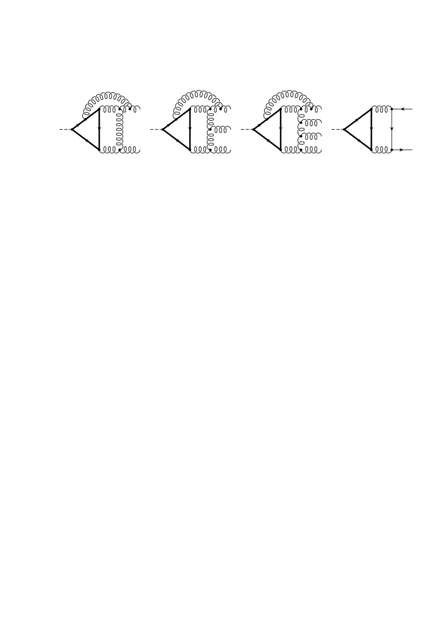
Figure 1: Typical Feynman diagrams contributing to the coefficients $\tilde{C}_{i}^{0}$ in Eq. (2). Looped, bold-faced, and dashed lines represent gluons, $t$ quarks, and $A$ bosons, respectively.

We now turn to the computation of the bare coefficient functions $\tilde{C}_{1}^{0}$ and $\tilde{C}_{2}^{0}$ in Eq. (2). We are thus led to consider irreducible vertex diagrams which connect one $A$ boson to the respective states of gluons and light-quark pairs via one or more $t$-quark loops, whereby all external particles are taken to be on their mass shells. Typical examples are depicted in Fig. 1. There are three independent ways to obtain $\tilde{C}_{1}^{0}$, namely from the sets of $ggA$ three-point, $gggA$ four-point, or $ggggA$ five-point diagrams. At the three-loop level, these sets contain 657, 7362, and 95004 diagrams, respectively. We choose to work out the first option in the covariant gauge with arbitrary gauge parameter, so that the gauge-parameter independence of the final result yields a nontrivial check. Another independent check is then provided by elaborating the second option in the ’t Hooft-Feynman gauge keeping only one external momentum different from zero. In order to cope with the enormous complexity of the problem at hand, we make successive use of powerful symbolic manipulation programs. Specifically, we generate and evaluate the contributing diagrams with the packages QGRAF [25] and MATAD [26], which is written in FORM [27], respectively. The cancellation of the UV singularities, the gauge-parameter independence, and the renormalization-group (RG) invariance serve as strong checks for our calculation.

Let us denote the sum of all relevant $ggA$ diagrams by $V_{ggA,\alpha\beta}^{\mu\nu\rho\sigma}(q_{1},q_{2})$, where $q_{1}$ and $q_{2}$ are the incoming four-momenta of the two on-shell gluons with polarization four-vectors $\epsilon_{1}^{\alpha}$ and $\epsilon_{2}^{\beta}$, respectively. According to Eq. (4), $V_{ggA,\alpha\beta}^{\mu\nu\rho\sigma}$ is by construction totally antisymmetric in the indices $\mu$, $\nu$, $\rho$, and $\sigma$. In order to compute $\tilde{C}_{1}^{0}$, we need to expand $V_{ggA}$ up to terms linear in $q_{1}$ and $q_{2}$. There is just one possible structure, namely

$$V_{ggA,\alpha\beta}^{\mu\nu\rho\sigma}(q_{1},q_{2})=C_{ggA}P_{ggA,\alpha\beta}^{\mu\nu\rho\sigma}(q_{1},q_{2}),\qquad P_{ggA,\alpha\beta}^{\mu\nu\rho\sigma}(q_{1},q_{2})=q_{1}^{[\mu}q_{2}^{\nu}g_{\alpha}^{\rho}g_{\beta}^{\sigma]},$$ (10)

so that the coefficient $C_{ggA}$ may be conveniently extracted by noting that $P_{ggA}^{2}=-(D-2)(D-3)(q_{1}\cdot q_{2})^{2}/24$. The final formula for $\tilde{C}_{1}^{0}$ reads

$$\tilde{C}_{1}^{0}=-\frac{3}{(D-2)(D-3)(q_{1}\cdot q_{2})^{2}}\,\frac{Z_{\rm MS}^{\rm p}Z_{5}^{\rm p}}{Z_{m}\zeta_{3}^{0}}P_{ggA,\mu\nu\rho\sigma}^{\alpha\beta}(q_{1},q_{2})V_{ggA,\alpha\beta}^{\mu\nu\rho\sigma}(q_{1},q_{2}).$$ (11)

The normalization of Eq. (11) may be understood as follows. On the one hand, we need to renormalize the mass and the pseudoscalar current of the $t$ quark in the Lagrangian (1) of the $n_{f}$-flavour theory. In this way, the renormalization constants $Z_{m}$ [28], $Z_{\rm MS}^{\rm p}$, and $Z_{5}^{\rm p}$ [23] enter. They are defined as

$$m_{t}^{0} = Z_{m}m_{t},$$

$$\left[\bar{t}\gamma_{5}t\right] = Z_{\rm MS}^{\rm p}Z_{5}^{\rm p}\bar{t}^{0}\gamma_{5}t^{0},$$ (12)

and read [23, 28]

$$Z_{m} = 1+\frac{\alpha_{s}^{(n_{f})}(\mu)}{\pi}\,\frac{1}{\varepsilon}\left(-\frac{3}{4}C_{F}\right)+\left(\frac{\alpha_{s}^{(n_{f})}(\mu)}{\pi}\right)^{2}\left[\frac{1}{\varepsilon^{2}}\left(\frac{9}{32}C_{F}^{2}+\frac{11}{32}C_{F}C_{A}-\frac{1}{8}C_{F}Tn_{f}\right)\right.$$

$${}+\left.\frac{1}{\varepsilon}\left(-\frac{3}{64}C_{F}^{2}-\frac{97}{192}C_{F}C_{A}+\frac{5}{48}C_{F}Tn_{f}\right)\right],$$

$$Z_{\rm MS}^{\rm p} = 1+\frac{\alpha_{s}^{(n_{f})}(\mu)}{\pi}\,\frac{1}{\varepsilon}\left(-\frac{3}{4}C_{F}\right)+\left(\frac{\alpha_{s}^{(n_{f})}(\mu)}{\pi}\right)^{2}\left[\frac{1}{\varepsilon^{2}}\left(\frac{9}{32}C_{F}^{2}+\frac{11}{32}C_{F}C_{A}-\frac{1}{8}C_{F}Tn_{f}\right)\right.$$

$${}+\left.\frac{1}{\varepsilon}\left(-\frac{3}{64}C_{F}^{2}+\frac{79}{192}C_{F}C_{A}-\frac{11}{48}C_{F}Tn_{f}\right)\right],$$

$$Z_{5}^{\rm p} = 1+\frac{\alpha_{s}^{(n_{f})}(\mu)}{\pi}(-2C_{F})+\left(\frac{\alpha_{s}^{(n_{f})}(\mu)}{\pi}\right)^{2}\left(\frac{1}{72}C_{F}C_{A}+\frac{1}{18}C_{F}Tn_{f}\right).$$ (13)

The finite renormalization constant $Z_{5}^{\rm p}$ is needed in addition to the usual UV renormalization constant of the $\overline{\rm MS}$ scheme, $Z_{\rm MS}^{\rm p}$, to effectively restore the anticommutativity of the $\gamma_{5}$ matrix [23, 29]. On the other hand, we need to express the bare couplings and fields appearing in the Lagrangian (2) of the $n_{l}$-flavour theory in terms of their counterparts in the $n_{f}$-flavour theory. The appropriate relations,

$$g_{s}^{0\prime}=\zeta_{g}^{0}g_{s}^{0},\qquad q_{i}^{0\prime}=\sqrt{\zeta_{2}^{0}}q_{i}^{0},\qquad G_{\mu}^{0\prime,a}=\sqrt{\zeta_{3}^{0}}G_{\mu}^{0,a},$$ (14)

involve the decoupling constants $\zeta_{g}^{0}$, $\zeta_{2}^{0}$, and $\zeta_{3}^{0}$. In the case of the $ggA$ amplitude, only $\zeta_{3}^{0}$ occurs. For our purposes, we need $\zeta_{3}^{0}$ through ${\cal O}(\varepsilon^{2}\alpha_{s})$ and ${\cal O}(\varepsilon\alpha_{s}^{2})$. The corresponding expression may be extracted from Eq. (B.2) of Ref. [11], where the renormalized version, $\zeta_{3}$, is listed through ${\cal O}(\alpha_{s}^{3})$ in the covariant gauge. Finally, a factor of 8 stems from the Feynman rule for the two-gluon piece of $\tilde{O}_{1}^{\prime}$. In Eq. (11), we may take the limit $q_{1},q_{2}\to 0$, which reduces the problem of finding $\tilde{C}_{1}^{0}$ to the solution of massive vacuum integrals [30]. After renormalization according to Eq. (9), we find

$$\tilde{C}_{1}=-\frac{\alpha_{s}^{(n_{l})}(\mu)}{\pi}\,\frac{T}{8}\left[1+0\cdot\frac{\alpha_{s}^{(n_{l})}(\mu)}{\pi}+0\cdot\left(\frac{\alpha_{s}^{(n_{l})}(\mu)}{\pi}\right)^{2}\right],$$ (15)

i.e. the correction terms of ${\cal O}(\alpha_{s})$ and ${\cal O}(\alpha_{s}^{2})$ indeed vanish, as was suggested in Ref. [7, 14] on the basis of the nonabelian variant [17] of the Adler-Bardeen theorem [15], which predicts that $\tilde{C}_{1}$ does not receive QCD corrections. Notice that this is only true if $\tilde{C}_{1}$ is expanded in $\alpha_{s}^{(n_{l})}(\mu)$.

As an independent check, we may also extract $\tilde{C}_{1}^{0}$ from the sum $V_{gggA,\alpha\beta\gamma}^{\mu\nu\rho\sigma}(q)$ of the $gggA$ diagrams, where $\alpha$, $\beta$, and $\gamma$ are the Lorentz indices of the gluon polarization four-vectors. Notice that it is sufficient to keep one external four-momentum, $q$, different from zero, since the three-gluon piece of $\tilde{O}_{1}^{\prime}$ contains just one derivative. Again, there is only one possible structure linear in $q$, namely

$$V_{gggA,\alpha\beta\gamma}^{\mu\nu\rho\sigma}(q)=C_{gggA}P_{gggA,\alpha\beta\gamma}^{\mu\nu\rho\sigma}(q),\qquad P_{gggA,\alpha\beta\gamma}^{\mu\nu\rho\sigma}(q)=q^{[\mu}g_{\alpha}^{\nu}g_{\beta}^{\rho}g_{\gamma}^{\sigma]},$$ (16)

so that the coefficient $C_{gggA}$ may be easily extracted by using $P_{gggA}^{2}=(D-1)(D-2)(D-3)q^{2}/24$. In contrast to the two-gluon piece of $\tilde{O}_{1}^{\prime}$, we now have to include decoupling constants for three gluon fields and one gauge coupling. Again, the Feynman rule for the three-gluon piece of $\tilde{O}_{1}^{\prime}$ involves a factor of 8. Thus, the final formula for $\tilde{C}_{1}^{0}$ is given by

$$\tilde{C}_{1}^{0}=\frac{3}{(D-1)(D-2)(D-3)q^{2}}\,\frac{Z_{\rm MS}^{\rm p}Z_{5}^{\rm p}}{Z_{m}\zeta_{g}^{0}(\zeta_{3}^{0})^{3/2}}P_{gggA,\mu\nu\rho\sigma}^{\alpha\beta\gamma}(q)V_{gggA,\alpha\beta\gamma}^{\mu\nu\rho\sigma}(q).$$ (17)

Taking the limit $q\to 0$ and and working in the ’t Hooft-Feynman gauge, we recover from Eq. (17) our previous result for $\tilde{C}_{1}^{0}$.

Finally, we turn to $\tilde{C}_{2}^{0}$, which is generated by vertex diagrams that couple the $A$ boson to a pair of light quarks and involve a virtual $t$ quark. This requires at least two loops. Specifically, there are 2 two-loop and 63 three-loop diagrams of this type. Calling the resulting $q_{i}\bar{q}_{i}A$ amplitude $V_{qqA}^{\mu\nu\rho\sigma}(q)$, where the argument $q$ is the incoming four-momentum of the $A$ boson, we may extract $\tilde{C}_{2}^{0}$ as

$$\tilde{C}_{2}^{0}=\frac{6}{(D-1)(D-2)(D-3)q^{2}}\,\frac{Z_{\rm MS}^{\rm p}Z_{5}^{\rm p}}{Z_{m}\zeta_{2}^{0}}{\rm Tr}\,\left[q_{\mu}\gamma_{\nu}\gamma_{\rho}\gamma_{\sigma}V_{qqA}^{\mu\nu\rho\sigma}(q)\right].$$ (18)

In order to treat the $A\to gg$ decay at three loops, it is sufficient to know the leading term of $\tilde{C}_{2}$. Moreover, due to Eq. (9), the computation of the next-to-leading term of $\tilde{C}_{2}$ would require the knowledge of $Z_{12}^{\prime}$ to ${\cal O}(\alpha_{s}^{2})$, which is not yet available. After renormalization according to Eq. (9), we find

$$\tilde{C}_{2}=\left(\frac{\alpha_{s}^{(n_{l})}(\mu)}{\pi}\right)^{2}C_{F}T\left(\frac{3}{16}-\frac{3}{8}\ln\frac{\mu^{2}}{m_{t}^{2}(\mu)}\right),$$ (19)

where $m_{t}(\mu)$ is the $\overline{\rm MS}$ mass of the $t$ quark.

3 $A\to gg$ decay

Having established the high-$m_{t}$ effective Lagrangian (5) controlling the QCD interactions of the $A$ boson, we are now in a position to evaluate from it the ${\cal O}(\alpha_{s}^{2})$ correction to the $A\to gg$ decay width. To this end, we need to compute the absorptive part of the $A$-boson self-energy, at $q^{2}=M_{A}^{2}$, induced by $[\tilde{O}_{1}^{\prime}]$ and $[\tilde{O}_{2}^{\prime}]$ to sufficiently high order in the $n_{l}$-flavour theory.

In $D$ dimensions, the correlator function, at four-momentum $q$, of two bare operators of the type defined in Eq. (4) has the Lorentz decomposition

$$\left\langle\tilde{O}_{i,\mu\nu\rho\sigma}^{\prime}\tilde{O}_{j}^{\prime,\mu^{\prime}\nu^{\prime}\rho^{\prime}\sigma^{\prime}}\right\rangle=\Pi_{1,ij}^{0}(q^{2})q^{2}g_{[\mu}^{[\mu^{\prime}}g_{\nu}^{\nu^{\prime}}g_{\rho}^{\rho^{\prime}}g_{\sigma]}^{\sigma^{\prime}]}+\Pi_{2,ij}^{0}(q^{2})q_{[\mu}q^{[\mu^{\prime}}g_{\nu}^{\nu^{\prime}}g_{\rho}^{\rho^{\prime}}g_{\sigma]}^{\sigma^{\prime}]},$$ (20)

where $\Pi_{1,ij}^{0}$ and $\Pi_{2,ij}^{0}$ are functions of $q^{2}$. We may extract $\Pi_{1,ij}^{0}$ and $\Pi_{2,ij}^{0}$ by totally contracting Eq. (20) with the projectors

$$P_{1,\mu\nu\rho\sigma}^{\mu^{\prime}\nu^{\prime}\rho^{\prime}\sigma^{\prime}}(q) = \frac{24}{(q^{2})^{2}}\,\frac{\left(q^{2}g_{[\mu}^{[\mu^{\prime}}g_{\nu}^{\nu^{\prime}}g_{\rho}^{\rho^{\prime}}g_{\sigma]}^{\sigma^{\prime}]}-4q_{[\mu}q^{[\mu^{\prime}}g_{\nu}^{\nu^{\prime}}g_{\rho}^{\rho^{\prime}}g_{\sigma]}^{\sigma^{\prime}]}\right)}{(D-1)(D-2)(D-3)(D-4)},$$

$$P_{2,\mu\nu\rho\sigma}^{\mu^{\prime}\nu^{\prime}\rho^{\prime}\sigma^{\prime}}(q) = \frac{96}{(q^{2})^{2}}\,\frac{\left(-q^{2}g_{[\mu}^{[\mu^{\prime}}g_{\nu}^{\nu^{\prime}}g_{\rho}^{\rho^{\prime}}g_{\sigma]}^{\sigma^{\prime}]}+Dq_{[\mu}q^{[\mu^{\prime}}g_{\nu}^{\nu^{\prime}}g_{\rho}^{\rho^{\prime}}g_{\sigma]}^{\sigma^{\prime}]}\right)}{(D-1)(D-2)(D-3)(D-4)},$$ (21)

respectively. Notice that $P_{1}$ and $P_{2}$ develop $1/\varepsilon$ poles in the physical limit $\varepsilon\to 0$. This may be understood by observing that the two terms on the right-hand side of Eq. (20) are actually linearly dependent in four dimensions. In practice, the appearance of $1/\varepsilon$ poles in Eq. (21) does not create a problem, since we are only interested in the absorptive parts of the correlators in Eq. (20), so that it suffices to extract the pole parts of the relevant diagrams. It turns out that $\Pi_{1,ij}^{0}=0$, so that, after performing renormalization, taking the physical limit $\varepsilon\to 0$, and contracting with the Levi-Civita tensors, we have

$$\left\langle\left[\tilde{O}_{i}^{\prime}\right]\left[\tilde{O}_{j}^{\prime}\right]\right\rangle=-6q^{2}\Pi_{2,ij}(q^{2}),$$ (22)

where $\Pi_{2,ij}$ is the renormalized version of $\Pi_{2,ij}^{0}$. In fact, it can be shown that $\Pi_{1,ij}^{0}$ vanishes on kinematical grounds. As is well known, $\tilde{O}_{1}^{\prime}$ can be written as the divergence of the so-called Chern-Simons current, $K^{\prime,\mu}=\epsilon^{\mu\nu\rho\sigma}K_{\nu\rho\sigma}^{\prime}$ with $K_{\nu\rho\sigma}^{\prime}=4G_{\nu}^{0\prime,a}\partial_{\rho}G_{\sigma}^{0\prime,a}+(4/3)g_{s}^{0\prime}f^{abc}G_{\nu}^{0\prime,a}G_{\rho}^{0\prime,b}G_{\sigma}^{0\prime,c}$, i.e. $\tilde{O}_{1}^{\prime}=\partial_{\mu}K^{\prime,\mu}$, which is an exact identity. This implies that $\tilde{O}_{1,\mu\nu\rho\sigma}^{\prime}=\partial_{[\mu}K_{\nu\rho\sigma]}^{\prime}$. Thus, the correlator in Eq. (20) is represented by just one term proportional to $q_{[\mu}q^{[\mu^{\prime}}\langle K_{\nu\rho\sigma]}^{\prime}K^{\prime,\nu^{\prime}\rho^{\prime}\sigma^{\prime}]}\rangle$, whence it follows that $\Pi_{1,ij}^{0}=0$.

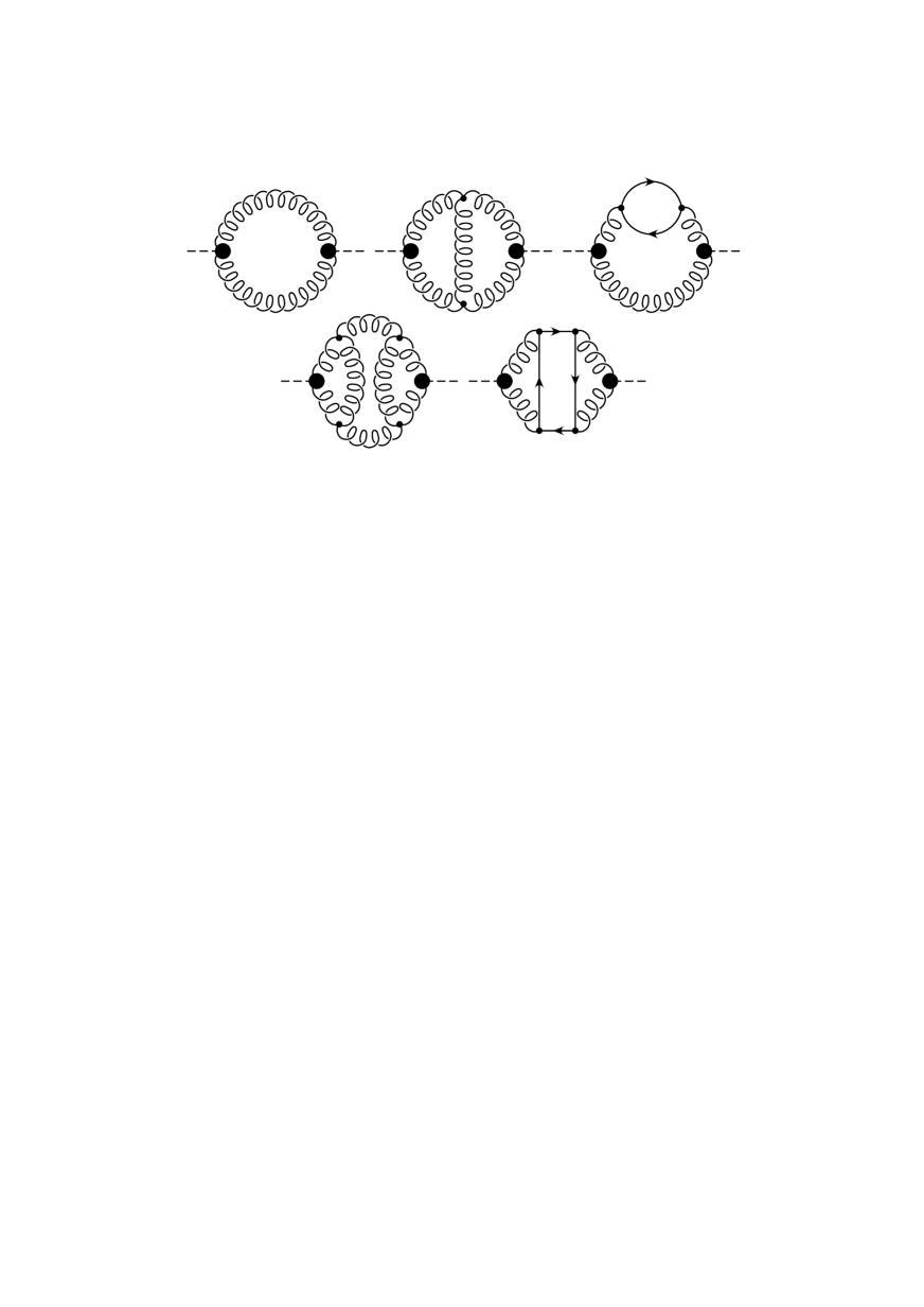
Figure 2: Typical Feynman diagrams contributing to the correlator $\langle\tilde{O}_{1}^{\prime}\tilde{O}_{1}^{\prime}\rangle$. Looped, solid, and dashed lines represent gluons, light quarks, and $A$ bosons, respectively. Solid circles represent insertions of $\tilde{O}_{1}^{\prime}$.

Due to Eq. (6), all three correlators $\langle\tilde{O}_{1}^{\prime}\tilde{O}_{1}^{\prime}\rangle$, $\langle\tilde{O}_{1}^{\prime}\tilde{O}_{2}^{\prime}\rangle$, and $\langle\tilde{O}_{2}^{\prime}\tilde{O}_{2}^{\prime}\rangle$ contribute to $\langle[\tilde{O}_{1}^{\prime}][\tilde{O}_{1}^{\prime}]\rangle$, the absorptive part of which we wish to calculate through ${\cal O}(\alpha_{s}^{2})$. At the three-loop level, these three correlators receive contributions from $403$, $28$, and $33$ massless diagrams, respectively. Typical examples pertaining to $\langle\tilde{O}_{1}^{\prime}\tilde{O}_{1}^{\prime}\rangle$ are depicted in Fig. 2. We generate and evaluate the contributing diagrams with the packages QGRAF [25] and MINCER [31], which is written in FORM [27]. We work in the covariant gauge with arbitrary gauge parameter. The cancellation of the latter in the final results serves as a welcome check.

Our results for the absorptive parts of the renormalized correlators read

$${\rm Im}\,\left\langle\left[\tilde{O}_{1}^{\prime}\right]\left[\tilde{O}_{1}^{\prime}\right]\right\rangle = \frac{(q^{2})^{2}}{\pi}N_{A}\left\{1+\frac{\alpha_{s}^{(n_{l})}(\mu)}{\pi}\left[C_{A}\left(\frac{97}{12}+\frac{11}{6}\ln\frac{\mu^{2}}{q^{2}}\right)+Tn_{l}\left(-\frac{7}{3}\right.\right.\right.$$

$${}-\left.\left.\frac{2}{3}\ln\frac{\mu^{2}}{q^{2}}\right)\right]+\left(\frac{\alpha_{s}^{(n_{l})}(\mu)}{\pi}\right)^{2}\left[C_{A}^{2}\left(\frac{51959}{864}-\frac{121}{24}\zeta(2)-\frac{55}{8}\zeta(3)\right.\right.$$

$${}+\left.\frac{1135}{48}\ln\frac{\mu^{2}}{q^{2}}+\frac{121}{48}\ln^{2}\frac{\mu^{2}}{q^{2}}\right)+C_{F}Tn_{l}\left(-\frac{107}{12}+3\zeta(3)-2\ln\frac{\mu^{2}}{q^{2}}\right)$$

$${}+C_{A}Tn_{l}\left(-\frac{3793}{108}+\frac{11}{3}\zeta(2)-\frac{1}{2}\zeta(3)-\frac{46}{3}\ln\frac{\mu^{2}}{q^{2}}-\frac{11}{6}\ln^{2}\frac{\mu^{2}}{q^{2}}\right)$$

$${}+\left.\left.T^{2}n_{l}^{2}\left(\frac{251}{54}-\frac{2}{3}\zeta(2)+\frac{7}{3}\ln\frac{\mu^{2}}{q^{2}}+\frac{1}{3}\ln^{2}\frac{\mu^{2}}{q^{2}}\right)\right]\right\}$$

$$= \frac{(q^{2})^{2}}{\pi}8\left\{1+\frac{\alpha_{s}^{(n_{l})}(\mu)}{\pi}\left[\frac{97}{4}+\frac{11}{2}\ln\frac{\mu^{2}}{q^{2}}+n_{l}\left(-\frac{7}{6}-\frac{1}{3}\ln\frac{\mu^{2}}{q^{2}}\right)\right]\right.$$

$${}+\left(\frac{\alpha_{s}^{(n_{l})}(\mu)}{\pi}\right)^{2}\left[\frac{51959}{96}-\frac{363}{8}\zeta(2)-\frac{495}{8}\zeta(3)+n_{l}\left(-\frac{469}{8}+\frac{11}{2}\zeta(2)\right.\right.$$

$${}+\left.\frac{5}{4}\zeta(3)\right)+n_{l}^{2}\left(\frac{251}{216}-\frac{1}{6}\zeta(2)\right)+\left(\frac{3405}{16}-\frac{73}{3}n_{l}+\frac{7}{12}n_{l}^{2}\right)\ln\frac{\mu^{2}}{q^{2}}$$

$${}+\left.\left.\left(\frac{363}{16}-\frac{11}{4}n_{l}+\frac{1}{12}n_{l}^{2}\right)\ln^{2}\frac{\mu^{2}}{q^{2}}\right]\right\},$$

$${\rm Im}\,\left\langle\left[\tilde{O}_{1}^{\prime}\right]\left[\tilde{O}_{2}^{\prime}\right]\right\rangle = \frac{(q^{2})^{2}}{\pi}\,\frac{\alpha_{s}^{(n_{l})}(\mu)}{\pi}\left(\frac{N_{A}Tn_{l}}{4}\right),$$

$${\rm Im}\,\left\langle\left[\tilde{O}_{2}^{\prime}\right]\left[\tilde{O}_{2}^{\prime}\right]\right\rangle = \frac{(q^{2})^{2}}{\pi}\left(\frac{\alpha_{s}^{(n_{l})}(\mu)}{\pi}\right)^{2}\left(\frac{N_{A}T^{2}n_{l}^{2}}{16}\right),$$ (23)

where $\zeta$ is Riemann’s zeta function, with values $\zeta(2)=\pi^{2}/6$ and $\zeta(3)\approx 1.202\,057$, and we have put $N_{c}=3$ in the second expression on the right-hand side. Notice that ${\rm Im}\,\langle[\tilde{O}_{2}^{\prime}][\tilde{O}_{2}^{\prime}]\rangle$ starts at ${\cal O}(\alpha_{s}^{2})$. This may be understood by observing that the $A\to q_{i}\bar{q}_{i}$ decay width is helicity suppressed and quenched if the quark $q_{i}$ is taken to be massless. Thus, in order for a diagram to contribute it must have a cut which only involves gluons. Such diagrams first appear at three loops. Actually, the results in Eq. (23) are not mutually independent. In fact, Eq. (7) allows us to derive ${\rm Im}\,\langle[\tilde{O}_{1}^{\prime}][\tilde{O}_{2}^{\prime}]\rangle$ and ${\rm Im}\,\langle[\tilde{O}_{2}^{\prime}][\tilde{O}_{2}^{\prime}]\rangle$ from ${\rm Im}\,\langle[\tilde{O}_{1}^{\prime}][\tilde{O}_{1}^{\prime}]\rangle$ and thus provides a welcome check for Eq. (23). The ${\cal O}(\alpha_{s})$ term of ${\rm Im}\,\langle[\tilde{O}_{1}^{\prime}][\tilde{O}_{1}^{\prime}]\rangle$ in Eq. (23) is in agreement with Ref. [12].

All ingredients which enter the calculation of the $A\to gg$ decay width through ${\cal O}(\alpha_{s}^{4})$ are now available. From Eq. (5), we derive the general expression

$$\Gamma(A\to gg)=\frac{\sqrt{2}G_{F}}{M_{A}}\left(\tilde{C}_{1}^{2}{\rm Im}\,\left\langle\left[\tilde{O}_{1}^{\prime}\right]\left[\tilde{O}_{1}^{\prime}\right]\right\rangle+2\tilde{C}_{1}\tilde{C}_{2}{\rm Im}\,\left\langle\left[\tilde{O}_{1}^{\prime}\right]\left[\tilde{O}_{2}^{\prime}\right]\right\rangle+\tilde{C}_{2}^{2}{\rm Im}\,\left\langle\left[\tilde{O}_{2}^{\prime}\right]\left[\tilde{O}_{2}^{\prime}\right]\right\rangle\right),$$ (24)

where it is understood that the correlators are to be evaluated at $q^{2}=M_{A}^{2}$. The last term contained within the parenthesis of Eq. (24) contributes in ${\cal O}(\alpha_{s}^{6})$ and is only included for completeness. Inserting Eqs. (15) and (23) in Eq. (24) and putting $N_{c}=3$, $n_{l}=5$, and $\mu=M_{A}$, we finally obtain

$$\Gamma(A\to gg) = \frac{G_{F}M_{A}^{3}}{16\pi\sqrt{2}}\left(\frac{\alpha_{s}^{(5)}(M_{A})}{\pi}\right)^{2}\left[1+\frac{221}{12}\,\frac{\alpha_{s}^{(5)}(M_{A})}{\pi}+\left(\frac{\alpha_{s}^{(5)}(M_{A})}{\pi}\right)^{2}\right.$$ (25)

$${}\times\left.\left(\frac{237311}{864}-\frac{529}{24}\zeta(2)-\frac{445}{8}\zeta(3)-5\ln\frac{M_{t}^{2}}{M_{A}^{2}}\right)\right]$$

$$\approx \frac{G_{F}M_{A}^{3}}{16\pi\sqrt{2}}\left(\frac{\alpha_{s}^{(5)}(M_{A})}{\pi}\right)^{2}\left[1+18.417\,\frac{\alpha_{s}^{(5)}(M_{A})}{\pi}+\left(\frac{\alpha_{s}^{(5)}(M_{A})}{\pi}\right)^{2}\right.$$

$${}\times\left.\left(171.544-5\ln\frac{M_{t}^{2}}{M_{A}^{2}}\right)\right].$$

The ${\cal O}(\alpha_{s})$ correction in Eq. (25) agrees with the result originally found in Refs. [7, 12]. If we assume that $\alpha_{s}^{(5)}(M_{A})=0.116$, which follows from $\alpha_{s}^{(5)}(M_{Z})=0.118$ for $M_{A}=100$ GeV, and take the $t$-quark pole mass to be $M_{t}=175.6$ GeV, then the correction factor corresponding to the square bracket in Eq. (25) has the value $1+0.68+0.23=1.91$, i.e. the three-loop term amounts to 33% of the two-loop term. This is somewhat larger than the corresponding correction factor for a SM Higgs boson with mass $M_{H}=100$ GeV, which was found to be $1+0.66+0.21=1.87$ [10]. For our choice of input parameters, we obtain from Eq. (25) the QCD-corrected prediction $\Gamma(A\to gg)=426$ keV.

Similarly to the $H\to gg$ case [10], Eq. (25) may be RG improved by resumming the logarithms of the type $\ln(M_{t}^{2}/M_{A}^{2})$. This leads to

$$\Gamma(A\to gg) = \frac{G_{F}M_{A}^{3}}{16\pi\sqrt{2}}\left(\frac{\alpha_{s}^{(5)}(M_{A})}{\pi}\right)^{2}\left[1+\frac{4363}{276}\,\frac{\alpha_{s}^{(5)}(M_{A})}{\pi}+\frac{60}{23}\,\frac{\alpha_{s}^{(6)}(M_{t})}{\pi}\right.$$ (26)

$${}+\left(\frac{239471}{864}-\frac{529}{24}\zeta(2)-\frac{445}{8}\zeta(3)\right)\left(\frac{\alpha_{s}^{(5)}(M_{A})}{\pi}\right)^{2}$$

$${}-\left.\frac{1800}{529}\,\frac{\alpha_{s}^{(5)}(M_{A})}{\pi}\,\frac{\alpha_{s}^{(6)}(M_{t})}{\pi}+\frac{955}{1058}\,\left(\frac{\alpha_{s}^{(6)}(M_{t})}{\pi}\right)^{2}\right]$$

$$\approx \frac{G_{F}M_{A}^{3}}{16\pi\sqrt{2}}\left(\frac{\alpha_{s}^{(5)}(M_{A})}{\pi}\right)^{2}\left[1+15.808\,\frac{\alpha_{s}^{(5)}(M_{A})}{\pi}+2.609\,\frac{\alpha_{s}^{(6)}(M_{t})}{\pi}\right.$$

$${}+174.044\left(\frac{\alpha_{s}^{(5)}(M_{A})}{\pi}\right)^{2}-3.403\,\frac{\alpha_{s}^{(5)}(M_{A})}{\pi}\,\frac{\alpha_{s}^{(6)}(M_{t})}{\pi}$$

$${}+\left.0.903\left(\frac{\alpha_{s}^{(6)}(M_{t})}{\pi}\right)^{2}\right].$$

Since, at present, the experimental lower bound on $M_{A}$ in the MSSM is 24.3 GeV [32], we have $\ln(M_{t}^{2}/M_{A}^{2})<4$, so that the numerical effect of the RG improvement is negligible in practical applications.

It is interesting to compare the exact value of the ${\cal O}(\alpha_{s}^{2})$ correction in Eq. (25) with the estimates one may derive from the knowledge of the ${\cal O}(\alpha_{s})$ correction through the application of well-known scale-optimization procedures, based on the fastest apparent convergence (FAC) [33], the principle of minimal sensitivity (PMS) [34], and the proposal by Brodsky, Lepage, and Mackenzie (BLM) [35] to resum the leading light-quark contribution to the renormalization of the strong coupling constant. These procedures lead to the generic expression

$$\Gamma(A\to gg) = \frac{G_{F}M_{A}^{3}}{16\pi\sqrt{2}}\left(\frac{\alpha_{s}^{(5)}(\xi M_{A})}{\pi}\right)^{2}\left(1+\bar{K}_{1}\frac{\alpha_{s}^{(5)}(\xi M_{A})}{\pi}\right)$$ (27)

$$= \frac{G_{F}M_{A}^{3}}{16\pi\sqrt{2}}\left(\frac{\alpha_{s}^{(5)}(M_{A})}{\pi}\right)^{2}\left[1+K_{1}\frac{\alpha_{s}^{(5)}(M_{A})}{\pi}+\bar{K}_{2}\left(\frac{\alpha_{s}^{(5)}(M_{A})}{\pi}\right)^{2}\right],$$

where $K_{1}=k_{1}+n_{l}\kappa_{1}$, with $k_{1}=97/4$ and $\kappa_{1}=-7/6$, is the coefficient of the ${\cal O}(\alpha_{s})$ correction in Eq. (25). The FAC, PMS, and BLM expressions for $\xi$, $\bar{K}_{1}$, and $\bar{K}_{2}$ read

$$\ln\xi^{\rm FAC} = -\frac{K_{1}}{4\beta_{0}},\qquad\bar{K}_{1}^{\rm FAC}=0,\qquad\bar{K}_{2}^{\rm FAC}=K_{1}\left(\frac{3}{4}K_{1}+\frac{\beta_{1}}{\beta_{0}}\right),$$

$$\ln\xi^{\rm PMS} = -\frac{1}{2\beta_{0}}\left(\frac{K_{1}}{2}+\frac{\beta_{1}}{3\beta_{0}}\right),\qquad\bar{K}_{1}^{\rm PMS}=-\frac{2\beta_{1}}{3\beta_{0}},\qquad\bar{K}_{2}^{\rm PMS}=\frac{1}{3}\left(\frac{3}{2}K_{1}+\frac{\beta_{1}}{\beta_{0}}\right)^{2},$$

$$\ln\xi^{\rm BLM} = \frac{3}{2}\kappa_{1},\qquad\bar{K}_{1}^{\rm BLM}=k_{1}+\frac{33}{2}\kappa_{1},$$

$$\bar{K}_{2}^{\rm BLM} = \kappa_{1}\left[\frac{3}{4}\kappa_{1}n_{l}^{2}+\frac{1}{2}\left(3k_{1}+\frac{19}{2}\right)n_{l}-\frac{9}{4}\left(11k_{1}+\frac{363}{4}\kappa_{1}+17\right)\right],$$ (28)

respectively, where $\beta_{0}=11/4-n_{l}/6$ and $\beta_{1}=51/8-19n_{l}/24$ are the first two coefficients of the Callan-Symanzik beta function of QCD. The numerical results for $n_{l}=5$ are summarized in Table 1. The values of $\bar{K}_{2}$ should be compared with the true coefficient $K_{2}$ of the ${\cal O}(\alpha_{s}^{2})$ correction in Eq. (25). For completeness, we also list in Table 1 the corresponding results for the $H\to gg$ decay width. In this case, one has $K_{2}\approx 156.808-5.708\ln(M_{t}^{2}/M_{H}^{2})$ [10]. In both cases, all three scale-optimization prescriptions correctly predict the sign and the order of magnitude of $K_{2}$. Furthermore, the three $\bar{K}_{2}$ values for the $H\to gg$ decay width are indeed smaller than the respective values for the $A\to gg$ case. Similarly to Ref. [36], the FAC and PMS results almost coincide.

Table 1: Numerical evaluation of Eq. (28) with $n_{l}=5$ for the $A\to gg$ and $H\to gg$ decay widths.

	$A\to gg$			$H\to gg$
	$\xi$	$\bar{K}_{1}$	$\bar{K}_{2}$	$\xi$	$\bar{K}_{1}$	$\bar{K}_{2}$
FAC	0.091	0	277.601	0.097	0	263.346
PMS	0.081	$-0.841$	278.131	0.087	$-0.841$	263.876
BLM	0.174	5	252.547	0.174	4.5	242.484

4 Discussion and conclusions

In this paper, we studied the interactions of a neutral CP-odd scalar boson $A$ with gluons and $n_{l}$ light quarks $q_{i}$ in the presence of a heavy quark $t$, with mass $m_{t}\gg M_{A}/2$, through three loops in QCD. For simplicity, we assumed that the Yukawa couplings of the light quarks may be neglected, which is a useful approximation in the 2HDM with $\tan\beta\approx 1$, where the Yukawa couplings and the masses of the quarks are related by a flavour-independent proportionality factor. Starting from the Yukawa Lagrangian (1) embedded in full QCD, we integrated out the $t$ quark to obtain the corresponding effective Lagrangian of the $n_{l}$-flavour theory, the renormalized version of which is given by Eq. (5). The operators in Eq. (5) comprise only light fields, while all residual dependence on the $t$ quark is contained in their coefficient functions. We diagrammatically evaluated the coefficients $\tilde{C}_{1}$ and $\tilde{C}_{2}$ of the physical operators $[\tilde{O}_{1}^{\prime}]$ and $[\tilde{O}_{2}^{\prime}]$ through ${\cal O}(\alpha_{s}^{3})$ and ${\cal O}(\alpha_{s}^{2})$, respectively. This is consistent, since $[\tilde{O}_{2}^{\prime}]$ is of ${\cal O}(\alpha_{s})$ relative to $[\tilde{O}_{1}^{\prime}]$ as may be seen from Eq. (7). We worked in the $\overline{\rm MS}$ renormalization scheme [20] with the convention that Eq. (7) should be exact [23]. Our results for $\tilde{C}_{1}$ and $\tilde{C}_{2}$ are given in Eqs. (15) and (19), respectively. In particular, we found that the ${\cal O}(\alpha_{s})$ and ${\cal O}(\alpha_{s}^{2})$ corrections to $\tilde{C}_{1}$ exactly vanish if the latter is expressed in terms of $\alpha_{s}^{(n_{l})}(\mu)$. We thus verified, by explicit calculation through three loops, the all-order prediction that $\tilde{C}_{1}$ does not receive any QCD corrections, which follows via a low-energy theorem [7, 14] from the nonabelian version [17] of the Adler-Bardeen non-renormalization theorem [15].

At this point, we should emphasize that, due to Eq. (7), the distinction between the renormalized operators $[\tilde{O}_{1}^{\prime}]$ and $[\tilde{O}_{2}^{\prime}]$ does not have a deep physical meaning. Actually, from Eqs. (5) and (7) it follows that the physical coupling of the $A$ boson to $[\tilde{O}_{1}^{\prime}]$ is proportional to $[\tilde{C}_{1}+\alpha_{s}^{(n_{l})}(\mu)Tn_{l}\tilde{C}_{2}/(4\pi)]$. Thus, the low-energy theorem gets violated starting from ${\cal O}(\alpha_{s}^{3})$ unless we stick to the $\overline{\rm MS}$ definitions of $[\tilde{O}_{1}^{\prime}]$ and $[\tilde{O}_{2}^{\prime}]$ [23].

The effective Lagrangian (5) allows us to evaluate physical observables related to the interactions of the $A$ boson with gluons and light quarks to higher orders in QCD by just considering massless diagrams in the $n_{l}$-flavour theory. As an application, we evaluated the ${\cal O}(\alpha_{s}^{2})$ correction to the $A\to gg$ decay width, extending the result of Refs. [7, 12] by one order. Our final result is listed in Eq. (25). For $M_{A}=100$ GeV, the overall QCD correction factor turned out to be as large as $1+0.68+0.23=1.91$. It is slightly larger than the corresponding correction factor for the $H\to gg$ decay width of the SM Higgs boson $H$ with the same mass, which was found to be $1+0.66+0.21=1.87$ [10]. The FAC [33], PMS [34], and BLM [35] predictions for the ${\cal O}(\alpha_{s}^{2})$ correction to the $A\to gg$ decay width are 0.38, 0.38, and 0.34, respectively. The corresponding results for the $H\to gg$ case are 0.36, 0.36, and 0.33.

Acknowledgements

We thank S.J. Brodsky and P.A. Grassi for useful discussions. W.A.B. and K.G.C. thank the MPI Theory Group for the hospitality extended to them during visits when the research reported here was initiated. B.A.K. thanks the NYU Physics Department for the hospitality extended to him during a visit when this manuscript was finalized. The work of K.G.C. was supported in part by INTAS under Contract INTAS–93–744–ext and by DFG under Contract KU 502/8–1.

References

• [1] M. Veltman, Nucl. Phys. B 123 (1977) 89.
• [2] H.M. Georgi, S.L. Glashow, M.E. Machacek and D.V. Nanopoulos, Phys. Rev. Lett. 40 (1978) 692.
• [3] V. Barger, M.S. Berger, A.L. Stange and R.J.N. Phillips, Phys. Rev. D 45 (1992) 4128;
J.F. Gunion and L.H. Orr, Phys. Rev. D 46 (1992) 2052;
J.F. Gunion, H.E. Haber and C. Kao, Phys. Rev. D 46 (1992) 2907;
Z. Kunszt and F. Zwirner, Nucl. Phys. B 385 (1992) 3.
• [4] F. Wilczek, Phys. Rev. Lett. 39 (1977) 1304.
• [5] S. Dawson, A. Djouadi and M. Spira, Phys. Rev. Lett. 77 (1996) 16.
• [6] S. Dawson, Nucl. Phys. B 359 (1991) 283;
A. Djouadi, M. Spira and P.M. Zerwas, Phys. Lett. B 264 (1991) 440;
D. Graudenz, M. Spira and P.M. Zerwas, Phys. Rev. Lett. 70 (1993) 1372;
M. Spira, A. Djouadi, D. Graudenz and P.M. Zerwas, Phys. Lett. B 318 (1993) 347;
S. Dawson and R. Kauffman, Phys. Rev. D 49 (1994) 2298;
M. Spira, Fortsch. Phys. 46 (1998) 203.
• [7] M. Spira, A. Djouadi, D. Graudenz and P.M. Zerwas, Nucl. Phys. B 453 (1995) 17.
• [8] M. Krämer, E. Laenen and M. Spira, Nucl. Phys. B 511 (1998) 523.
• [9] T. Inami, T. Kubota and Y. Okada, Z. Phys. C 18 (1983) 69.
• [10] K.G. Chetyrkin, B.A. Kniehl and M. Steinhauser, Phys. Rev. Lett. 79 (1997) 353.
• [11] K.G. Chetyrkin, B.A. Kniehl and M. Steinhauser, Nucl. Phys. B 510 (1998) 61.
• [12] A.L. Kataev, N.V. Krasnikov and A.A. Pivovarov, Nucl. Phys. B 198 (1982) 508; 490 (1997) 505 (E).
• [13] A. Djouadi, M. Spira, and P.M. Zerwas, Z. Phys. C 70 (1996) 427.
• [14] A. Djouadi, M. Spira and P.M. Zerwas, Phys. Lett. B 311 (1993) 255;
R.P. Kauffman and W. Schaffer, Phys. Rev. D 49 (1994) 551;
B.A. Kniehl and M. Spira, Z. Phys. C 69 (1995) 77.
• [15] S.L. Adler and W.A. Bardeen, Phys. Rev. 182 (1969) 1517;
R. Jackiw, Lectures on Current Algebra and its Applications, (Princeton University Press, New Jersey, 1972);
G. Bonneau, Nucl. Phys. B 171 (1980) 477;
J.C. Collins, Renormalization, (Cambridge University Press, Cambridge, 1984).
• [16] S.L. Adler, Phys. Rev. 177 (1969) 2416;
J. Bell and R. Jackiw, Nuovo Cimento 60 A (1969) 47.
• [17] W.A. Bardeen, in Proceedings of the Conference on Renormalization of Yang-Mills Fields and Applications to Particle Physics, Marseille, France, June 19–23, 1972, edited by C.P. Korthals-Altes, p. 29; in Proceedings of the XVI International Conference on High Energy Physics, Batavia, Illinois, September 6–13, 1972, edited by J.D. Jackson and A. Roberts, Vol. 2, p. 295;
A. Zee, Phys. Rev. Lett. 29 (1972) 1198;
J.H. Lowenstein and B. Schroer, Phys. Rev. D 7 (1973) 1929;
G. Bandelloni, C. Becchi, A. Blasi and R. Collina, Commun. Math. Phys. 72 (1980) 239;
M. Bos, Nucl. Phys. B 404 (1993) 215.
• [18] C.G. Bollini and J.J. Giambiagi, Phys. Lett. 40 B (1972) 566.
• [19] G. ’t Hooft and M. Veltman, Nucl. Phys. B 44 (1972) 189.
• [20] W.A. Bardeen, A.J. Buras, D.W. Duke and T. Muta, Phys. Rev. D 18 (1978) 3998.
• [21] G. ’t Hooft, Nucl. Phys. B 61 (1973) 455.
• [22] D.A. Akyeampong and R. Delbourgo, Nuovo Cimento 17 A (1973) 578.
• [23] S.A. Larin, Report No. NIKHEF–H/92–18 and hep–ph/9302240 (February 1993); Phys. Lett. B 303 (1993) 113.
• [24] D. Espriu and R. Tarrach, Z. Phys. C 16 (1982) 77;
P. Breitenlohner, D. Maison and K.S. Stelle, Phys. Lett. 134 B (1984) 63.
• [25] P. Nogueira, J. Comput. Phys. 105 (1993) 279.
• [26] M. Steinhauser, Ph.D. thesis, Karlsruhe University, (Shaker Verlag, Aachen, 1996).
• [27] J.A.M. Vermaseren, Symbolic Manipulation with FORM, (Computer Algebra Netherlands, Amsterdam, 1991).
• [28] R. Tarrach, Nucl. Phys. B 183 (1981) 384;
O.V. Tarasov, Dubna Report No. JINR P2–82–900 (1982);
N. Gray, D.J. Broadhurst, W. Grafe and K. Schilcher, Z. Phys. C 48 (1990) 673.
• [29] T.L. Trueman, Phys. Lett. 88 B (1979) 331.
• [30] S.G. Gorishny and S.A. Larin, Nucl. Phys. B 283 (1987) 452, and references cited therein.
• [31] S.A. Larin, F.V. Tkachev and J.A.M. Vermaseren, Report No. NIKHEF–H/91–18 (September 1991).
• [32] Particle Data Group, R.M. Barnett et al., Phys. Rev. D 54 (1996) 1.
• [33] G. Grunberg, Phys. Lett. 95 B (1980) 70; 110 B (1982) 501 (E); Phys. Rev. D 29 (1984) 2315.
• [34] P.M. Stevenson, Phys. Rev. D 23 (1981) 2916; Phys. Lett. 100 B (1981) 61; Nucl. Phys. B 203 (1982) 472; Phys. Lett. B 231 (1984) 65.
• [35] S.J. Brodsky, G.P. Lepage and P.B. Mackenzie, Phys. Rev. D 28 (1983) 228;
S.J. Brodsky and H.J. Lu, Phys. Rev. D 51 (1995) 3652.
• [36] K.G. Chetyrkin, B.A. Kniehl, and A. Sirlin, Phys. Lett. B 402 (1997) 359.