Next–to–Leading Order QCD corrections
to $B\overline{B}$–mixing and $\epsilon_{K}$ within the MSSM
F. Krauss, G. Soff

Institut f$\ddot{\rm u}$r Theoretische Physik

Technische Universit$\ddot{\rm a}$t Dresden

Mommsenstr.13, D-01062 Dresden, Germany

1 Introduction

During the last decade, Supersymmetry (SUSY) has been one of the most popular candidates for physics beyond the Standard Model (SM), see, e.g., the reviews [1]-[4]. Among all other ideas SUSY seemingly has the greatest potential to allow for the construction of a Grand Unified Theory. Even more, a low–energy version of SUSY would cancel the quadratic divergencies emerging within the Higgs–sector and cure the most nagging shortcomings of the Standard Model [5]-[9]. However, so far there is no experimental evidence for any of the new particles predicted by the various supersymmetric models up to scales of the order of the $W$– and $Z$–mass. So before the advent of the next generation of new colliders one probably has to rely on indirect probes to test the idea of a low–energy SUSY.

In this respect the most promising candidates are processes involving Flavour Changing Neutral Currents (FCNC), especially rare decays like $b\to s\gamma$ and oscillations in the system of neutral mesons, namely $B\overline{B}-$ and $K\overline{K}-$mixing [10]-[26]. In this paper we will focus on the latter class of processes and consider contributions to the mixing phenomena mediated by the chargino–squark and the charged Higgs–up–type quark sector of the Minimal Supersymmetric Standard Model (MSSM) taking into account gluonic Next–to–Leading Order QCD–corrections (NLO). We present results for the mass–splitting $\Delta M_{B}$ within the corresponding neutral $B$–system and for the parameter $\epsilon_{K}$ describing CP–violation in the $K$–system.

Within the framework of the SM the corresponding $\Delta F=2$ processes are governed by box–diagrams with internal up–type quarks and $W$–bosons and are suppressed by either small quark masses ($u$ and $c$) when compared to the $W$–mass or by small mixings between the third and the first two generations. The corresponding Leading Order diagrams of the SM are depicted in Fig. 1. The result for the SM up to NLO QCD corrections can be found in [27]-[30].

Within the MSSM – the supersymmetric extension of the SM with minimal field content, the same gauge group and soft symmetry breaking – there are different sources of flavour–changing processes. Nevertheless, all of them enter the stage of $\Delta F=2$ transitions via box–diagrams. First of all there are loops with internal up–type quarks and charged Higgs–Bosons (see Fig. 2). Taken alone, this corresponds to the Two Higgs Doublet Model (THDM), another popular extension of the SM. Results up to Next–to–Leading Order have been presented in [30]. The second source are loops involving charginos and up–type squarks (see Fig. 3). Their effect is investigated in this article up to NLO of gluonic QCD corrections. The last source of the $\Delta F=2$ processes within the MSSM are off–diagonal elements within the squark–mass matrices, entering via boxes containing down–type squarks and gluinos or neutralinos (see again Fig. 3). In the context of this paper we do not take into account their effect. Additionally we do not consider supersymmetric QCD–corrections mediated by gluinos although their effect might be sizable even in the limit of heavy gluinos [31]. The incorporation of these contributions would require additional extensive calculations which is beyond the scope of the current paper. In Leading Order the effect of the various MSSM–contributions on the mixing phenomena has been examined in [32]-[35]. There it is shown, that $K\overline{K}$–mixing strongly limits the size of some off–diagonal elements within the down–type squark matrix. Additionally, within the context of the mSUGRA model [36]-[39], LO–results have been presented in [40]. In this specific version of a supersymmetric extension of the SM, the soft supersymmetry–breaking terms are governed by just 5 parameters, reducing the vast number of parameters occuring within the MSSM considerably. The authors of [40] claim, that the most sizable contributions to $\Delta M_{B}$ and $\epsilon_{K}$ of the mSUGRA model in addition to the SM stem from the chargino–squark and the charged Higgs–up–type quark boxes when taking into account constraints of the parameter space as given by various other processes. These findings partly justify our focus on the charged Higgs– and the chargino–sector as primary sources of FCNC–processes.

It should be stressed here, that a priori the ratio of the vacuum expectation values of the two Higgs doublets, $\tan\!\beta$, is a free parameter. Overall fits to available experimental data constrain this parameter to two regions, $\tan\!\beta\approx 30-50$ and $\tan\!\beta\approx 1-2$, and it seems that the latter one is the more favourable one [41, 42, 43]. Here we will concentrate on this region of low $\tan\!\beta$, which yields the major contributions to the mixing phenomena as stated by [40].

The paper is organized as follows. After we redisplay the necessary parts of the MSSM–Feynman rules we shortly review the basic formalism in LO. In section 3 we discuss some features of the NLO calculations with special focus on the matching–procedure. In section 4 we provide the results in NLO for the different observables and scan to some extent the parameter space of the MSSM. We close with some concluding remarks.

2 Notation and basic formalism

2.1 Notation and Feynman–Rules

Throughout this paper we use the notation of [44]. Here it should be sufficient to list the relevant Feynman–rules and define the quantities involved. For the gauge bosons we employ the Feynman–t’Hooft gauge $\xi=1$, the propagators can be found in the Appendix. The relevant vertices are depicted in 1. There, the capital letters $I,J,K$ denote the quark generations, the letters $i,j$ label the squark–, Higgs– or chargino–fields and the $a,b,c$ are SU(3) indices in the appropriate representation. The matrices $Z^{\pm}$ and $Z_{U,D}$ diagonalize the mass matrices $X$ of the charginos and the up– and down–type squarks respectively,

$$(Z^{-})^{T}X_{\chi}Z^{+}=\mbox{\rm diag}(m_{\chi_{1,2}})\;\;,Z^{\dagger}_{U,D}X_{U,D}Z_{U,D}=\mbox{\rm diag}(m_{\tilde{u_{I}},\tilde{d_{I}}}),$$ (1)

Throughout this paper we will assume a specific form of the matrix $Z_{U}^{\pm}$ responsible for the mixing of the different squarks, namely all off–diagonal elements zero besides the ones associated with the mixing of the stops, $\tilde{u}^{3,6}$. Additionally, we assume the up–type squarks of the first two generations degenerate in mass. In other words, we assume, that the squark mass–matrix preserves flavour and mixes only the stops of different chiralities. This special form of the $Z$–matrices used in this paper is given in Eq. (39). It should be stressed here, that the last two assumptions concerning the up–type squark sector are mainly for the sake of a compact presentation but still somewhat unfounded. However, a generalization of our results to a more complicated structure of the up–type squark mass–matrix is quite straight–forward. It should be noted, that the four–squark vertex containing two up–type and two down–type squarks is not of relevance when considering ${\cal O}(\alpha_{s})$–corrections.

$C^{IJ}$ denotes the CKM–element between generations $I$ and $J$ and $\tan\!\beta=v_{2}/v_{1}$ is the ratio of the vacuum expectation values of the corresponding Higgs–doublets. We have explicitly written down the Yukawa–type couplings in terms of the quark masses involved. Simple inspection shows, that for the region of low $\tan\!\beta$ we can neglect the couplings proportional to the down–type masses with respect to the top–mass.

We use the short–hand notation

$$P_{L,R}=\frac{1\mp\gamma_{5}}{2}\,,\gamma^{\mu L}=\gamma^{\mu}P_{L}$$ (2)

for the left– and right–handed projectors and their combinations with gamma–matrices.

2.2 Leading Order

We want to summarize now briefly the ingredients used to obtain Leading Order results. In case of the $B\overline{B}$–mixing within the Standard Model this is quite transparent. Neglecting all masses besides the $W$– and the top–mass one can use the GIM–mechanism to account for the two lighter quark–types running in the boxes and calculate the remaining box–diagrams. This is simplified even more by using the Feynman–t’Hooft gauge for the $W$, leaving us with the physical $W$–boson and the would–be Goldstone–boson $\Phi$, both with identical masses. Results for boxes involving additional Higgs–bosons and top–quarks can be obtained in the same manner. Due to the fact that the supersymmetric partners of the SM–particles differ in Spin by $1/2$ one has to perform a Fierz–transformation for diagrams with squark– and chargino–lines to write down the emerging operator in terms of colour–singlet currents. As stated before, we assume, that the squarks of the first two generations ($\tilde{u}_{i}\,,i=1,2,4,5$) are degenerate in mass and do not mix considerably. This allows us to use the GIM–mechanism within the squark sector to tighten our final results. Generalization to non–degenerate squarks is straightforward.

The procedure of integrating out the heavy degrees of freedom leaves us with one operator and its Wilson–coefficient at the matching scale ${\mu_{0}}=O(M_{W}^{2})$ and yields the starting condition for the renormalization group equations. The connection between the starting scale and the bosonic scale $\mu=O(m_{B}^{2})$ is given in LO by the diagrams of Fig. 4 and a corresponding factor $\eta_{2}$. Putting everything together, the effective Hamiltonian for $\Delta B=2$–transitions at the bosonic scale is given by

$$H_{\rm{eff}}\;=\frac{1}{4}\,{G^{2}_{F}\over\pi^{2}}\;m_{W}^{2}\;{(V_{td}V^{\ast}_{tb})}^{2}\;\eta_{2}\;S\;{\cal O}_{LL}(\mu)\;,$$ (3)

where

$${\cal O}_{LL}=\left(\bar{d}_{i}\gamma_{\mu L}b_{i}\right)\;\left(\bar{d}_{j}\gamma^{\mu L}b_{j}\right)\;.$$ (4)

We have written out the colour indices for the quark fields explicitly. The coefficient $S$ is a sum of the well–known Inami–Lim functions [45] for the different internal particles,

$$S = S(x_{W},x_{H})+\tilde{S}(\{x_{i},y_{a}\})$$

$$S(x_{W},x_{H}) = S_{WW}(x_{W})+2\,S_{WH}(x_{W},x_{H})+S_{HH}(x_{H})\;.$$

$$\tilde{S}(\{x_{i},y_{a}\}) = \sum\limits_{i,j=1}^{2}\sum\limits_{a,b=1}^{6}\tilde{K}_{ij,ab}\tilde{S}(x_{i},x_{j},y_{a},y_{b})$$ (5)

Throughout this paper we use the following abbreviations

$$x_{W,H}=\frac{m_{t}^{2}}{M_{W,H}^{2}}\;,\;x_{d,s,c,b}=\frac{m_{d,s,c,b}^{2}}{M_{W}^{2}}\;,\;y_{a}=\frac{\tilde{m}_{\tilde{q}_{a}}^{2}}{M_{W}^{2}}\;,\;x_{i}=\frac{\tilde{m}_{\tilde{\chi}_{i}}^{2}}{M_{W}^{2}}$$ (6)

for the ratios of masses entering the Inami–Lim functions.

The $\tilde{K}$ in Eq. (2.2) account for the squark–quark–chargino couplings as given in the Feynman–rules above. They read

$$\tilde{K}_{ij,ab}=\prod\limits_{c=\{a,b\}}\prod\limits_{k=\{i,j\}}\left(Z_{U}^{Jc}Z_{1k}^{-}\frac{m_{u}^{J}}{\sqrt{2}M_{W}\sin\!\beta}Z_{U}^{(J+3)c}Z^{-}_{2k}\right)\,.$$ (7)

For the $K$–system the situation is slightly different. Because of the much lower mass of the $K$–meson, the charm–mass can not be neglected any more, and one has to account for this fact by integrating out the heavy degrees of freedom in consecutive steps [46]. So we end with a modified effective Hamiltonian for $\Delta S=2$–transitions at the bosonic scale, namely

$$H_{\rm{eff}} = \frac{1}{4}\,{G^{2}_{F}\over\pi^{2}}\;m_{W}^{2}\;\left[{(V_{cd}V^{\ast}_{cs})}^{2}\eta_{1}\,S(x_{c})+{(V_{td}V^{\ast}_{ts})}^{2}\eta_{2}\,S\right.$$ (8)

$$\;\;\;\;\;\;\;\;\;\;\;\;\;\;\;\;\;\;\;\left.+(V_{cd}V^{\ast}_{cs})(V_{td}V^{\ast}_{ts})\eta_{3}\,S(x_{c},x_{W})\right]\;{\cal O}_{LL}(\mu)\;,$$

where the contribution of the heavy particles alone, $S$ is given by Eq. (2.2) and the contributions involving a $c$–quark are contained in $S(x_{c})$ and $S(x_{c},x_{W})$ with corresponding QCD–correction factors $\eta_{1,3}$. Of course the operator ${\cal O}_{LL}$ changes accordingly, the $b$–quarks are replaced by strange quark fields.

The factors $\eta_{2\{B,K\}}$ in LO are given by [46]

$$\eta_{2B,LO} = \alpha_{s}(M_{W})^{\gamma^{(0)}/(2\beta^{(0)}_{5})}\;,\;$$

$$\eta_{2K,LO} = \alpha_{s}(m_{c})^{\gamma^{(0)}/(2\beta^{(0)}_{3})}\left(\frac{\alpha_{s}(m_{b})}{\alpha_{s}(m_{c})}\right)^{\gamma^{(0)}/(2\beta^{(0)}_{4})}\left(\frac{\alpha_{s}(M_{W})}{\alpha_{s}(m_{b})}\right)^{\gamma^{(0)}/(2\beta^{(0)}_{5})}\;,$$ (9)

where we have explicitly chosen the matching scale ${\mu_{0}}=M_{W}$. $\gamma^{(0)}$ and $\beta^{(0)}_{n_{f}}$ are the coefficents of the anomalous dimension of the operator ${\cal O}_{LL}$ and the QCD $\beta$–function in LO, the latter one is labelled by the number of active flavours, $n_{f}$. They are given by

$$\gamma^{(0)}=6\frac{N_{c}-1}{N_{c}}\;,\;\beta^{(0)}_{n_{f}}=\frac{11N_{c}-2n_{f}}{3}\;.$$ (10)

$N_{c}=3$ denotes the number of colours. We will see in the following, that we are able to plug the NLO QCD–corrections within the MSSM into the corresponding factor $\eta_{2}$, see Eqs. (3,8). The other QCD–factors $\eta_{1}$ and $\eta_{3}$ remain unaltered. Because they are even in LO quite complicated functions of $\alpha_{s}$, we just quote the numerical results for the NLO expressions we will use later,

$$\eta_{1}\approx 1.38\;,\;\eta_{3}\approx 0.47$$ (11)

as given in [29, 28].

The last task left is to extract the physically observable quantities from the effective Hamiltonians. In the case of the mass difference $\Delta M_{B}$ in the $B$–system and $\epsilon_{K}$ one has to sandwich the Hamiltonian in between two mesonic states. This amounts to the use of the relation

$$\langle\overline{B}|{\cal O}_{LL}(\mu)|B\rangle=\frac{2}{3}B_{B}(\mu)f_{B}^{2}m_{B}\,,$$ (12)

where the so–called bag–parameter is given scale–independently by

$$B_{B}=B_{B}(\mu)\alpha_{s}(\mu)^{g^{(0)}/(2\beta^{(0)}_{n_{f}})}\left[1-\frac{\alpha_{s}(\mu)}{4\pi}\,Z_{n_{f}}\right]\,.$$ (13)

Similar expressions hold for the $K$–system as well. In LO the last term of equation (13) can be omitted, the term $Z_{n_{f}}$ appearing there will be defined in the next section.

Unfortunately the evaluation of $B_{K}$ and $B_{B}f_{B}^{2}$ respectively by lattice calculations yields large uncertainties [29],

$$B_{K}=0.75\pm 0.15\;,\;\sqrt{B_{B}}f_{B}^{2}=0.2\pm 0.04\,\mbox{\rm GeV}\,,$$ (14)

and it is fair enough to state that this fact spoils the proper determination of the CKM–element $V_{td}$ by the processes considered here.

3 Explicit QCD–corrections, matching and running

3.1 Explicit QCD–corrections

We will now proceed by presenting the explicit perturbative QCD corrections up to $O(\alpha_{s})$. They are obtained by evaluating the diagrams in Figs.  5 and 6. For the diagrams containing quarks and bosons we performed the calculation in an arbitrary covariant $\xi$–gauge for the gluon and – as stated before – the Feynman–’tHooft gauge for the $W$–boson. For diagrams involving supersymmetric particles we chose explicitly $\xi=1$ for the gluon. Again, we perform a Fierz–transformation for the latter diagrams to write down the operators in terms of colour–singlett currents.

As one easily notices, diagrams (b,c,f,g,h) have the octet–structure $T_{a}\otimes T^{a}$ whereas the diagrams (a,d,e,j) have the singlet–structure ${\bf 1}\otimes{\bf 1}$. The double penguin diagrams (h) and the diagram (i) involving the four–squark coupling in a similar fashion do not contribute for vanishing external momenta.

Furthermore, we have to face ultraviolet as well as infrared divergencies. The first ones stem from the diagrams (d,e,j) . In this case we employ dimensional regularization within the so–called Naive Dimensional Regularization–scheme (NDR–scheme) [47, 28] and we renormalize using the $\overline{MS}$–scheme [47, 48]. Note, that for the supersymmetric particles we have to encounter additionally tadpole–like contribution (i) caused by the four–squark vertex. The infrared divergencies stem from the diagrams (a,b,c) . To handle them, we keep the masses of the external quarks whenever necessary. We will see, that this particular choice does not affect the final result for the Wilson–coefficient after performing the matching. Of course we could have used dimensional regularization as well, but the method chosen allows to compare the calculation presented here step by step with the ones presented earlier [27, 30].

In the following we will only consider the contribution to $\eta_{2}$, the parts of (8) involving the charm quark will not be displayed in this section. This reduces (8) to (3), and we will perform the necessary steps to gain $\eta_{2B}$ at NLO in this section before we just generalize on $\eta_{2K}$ at the end.

So the $O(\alpha_{s})$–corrections to the Hamiltonian of (3) show the structure

$$\Delta H_{\rm eff}=\frac{G_{F}^{2}}{4\pi^{2}}M_{W}^{2}\frac{\alpha_{s}}{4\pi}(V_{td}V_{tb}^{\ast})^{2}\,U\,,$$ (15)

with $U$ given by

$$U=\sum_{k}\left({\bf 1}\otimes{\bf 1}\,C_{F}\phi_{k}^{(1)}+T_{a}\otimes T^{a}\,\phi_{k}^{(8)}\right){\cal O}_{k}\,,$$ (16)

where a sum over $k=1,2,3,LL$ is performed. The operators ${\cal O}_{k}$ read

$${\cal O}_{LL} = \left(\bar{d}_{i}\gamma_{\mu L}b_{i}\right)\left(\bar{d}_{j}\gamma^{\mu L}b_{j}\right),$$

$${\cal O}_{1} = \left(\bar{d}_{i}P_{L}b_{i}\right)\left(\bar{d}_{j}P_{L}b_{j}\right)-\left(\bar{d}_{i}\sigma_{\mu\nu L}b_{i}\right)\left(\bar{d}_{j}\sigma^{\mu\nu L}b_{j}\right)+\{L\leftrightarrow R\}\,,$$

$${\cal O}_{2} = \left(\bar{d}_{i}P_{R}b_{i}\right)\left(\bar{d}_{j}P_{L}b_{j}\right)+\{L\leftrightarrow R\}\,,$$

$${\cal O}_{2} = \left(\bar{d}_{i}\gamma_{\mu R}b_{i}\right)\left(\bar{d}_{j}\gamma^{\mu L}b_{j}\right)+\{L\leftrightarrow R\}\,.$$ (17)

The operators ${\cal O}_{1,2,3}$ stem from the infrared divergent diagrams b,c and a, respectively. All of them are written in a Fierz–invariant fashion, allowing us to perform the Fierz–transformation for the supersymmetric contributions.

The colour factor $C_{F}$ along with $\tilde{C}_{A}$ to be used later is given by

$$C_{F}=\frac{N_{c}^{2}-1}{2N_{c}}\;,\;\tilde{C}_{A}=\frac{N_{c}-1}{2N_{c}}\,.$$ (18)

In analogy to Eq. (2.2) the functions $\phi$ can be decomposed as

$$\phi_{j}^{(i)}=\chi_{j}^{(i)}(x_{W},x_{H})+\tilde{\chi}_{j}^{(i)}(\{x_{i},y_{a}\})$$ (19)

for the parts involving quarks and bosons and the parts with squarks and charginos, respectively. The functions $\chi_{j}^{(i)}(x_{W},x_{H})$ have been calculated already [27, 30], here we just restate the result

$$\chi^{(1)}_{LL}(x_{W},x_{H}) = L^{(1,THDM)}(x_{W},xH)$$

$$+\left[2\xi\left(1+g_{IR}+\ln(x_{\mu_{0}})\right)+6\ln(x_{\mu_{0}})\sum_{i=H,W}\frac{x_{i}\partial}{\partial x_{i}}\right]\,S(x_{W},x_{H})\,,$$

$$\chi^{(8)}_{LL}(x_{W},x_{H}) = L^{(8,THDM)}(x_{W},xH)$$

$$+\left[2\xi\left(1+g_{IR}\right)+(3+\xi)\ln(x_{b}x_{d})\right]\,S(x_{W},x_{H})\,,$$

$$\chi_{1}^{(8)}(x_{W},x_{H}) = -(3+\xi)\,S(x_{W},x_{H})\,,$$

$$\chi_{2}^{(8)}(x_{W},x_{H}) = -2\chi_{3}^{(1)}(x_{W},x_{H})=-(3+\xi)\frac{m_{b}m_{d}}{m_{d}^{2}-m_{b}^{2}}\ln\left(\frac{x_{b}}{x_{d}}\right)\,S(x_{W},x_{H})\,.$$ (20)

All other $\chi$ equal zero. We have introduced here some other abbreviations,

$$x_{\mu_{0}}=\frac{{\mu_{0}}^{2}}{M_{W}^{2}}\;,\;g_{IR}=-\frac{x_{d}\ln(x_{d})-x_{b}\ln(x_{b})}{x_{d}-x_{b}}\,,$$ (21)

where ${\mu_{0}}$ is the scale of integrating out the heavy degrees of freedom. Note, that all masses entering the functions are the masses taken at this scale, for example, $m_{t}$ is the top–mass renormalized within the $\overline{MS}$–scheme at the scale ${\mu_{0}}$.

For the squarks and charginos running in the boxes the functions $\tilde{\chi}$ differ only slightly from the $\chi$ just presented. Namely, for the $\tilde{\chi}_{1,2,3}$ one just has to replace $S(x_{W},x_{H})$ by $\tilde{S}(\{x_{i},y_{a}\})$. The $\tilde{\chi}_{LL}$ read for $\xi=1$

$$\tilde{\chi}^{(1)}_{LL}(\{x_{i},y_{a}\}) = \sum\limits_{i,j=1}^{2}\sum\limits_{a,b=1}^{6}\tilde{K}_{ij,ab}\left\{\tilde{L}^{(1)}(x_{i,j},y_{a,b})\vphantom{\frac{|}{|}}+\left[2\left(1+g_{IR}+\ln(x_{\mu_{0}})\right)\right.\right.$$

$$\;\;\;\;\;\;\;\;\;\;\;\;\;\;\;\;\;\;\;\;\;\;\;\;+\left.\left.2\ln(x_{\mu_{0}})\sum_{k=i,j}\sum_{c=a,b}\left(\frac{3x_{i}\partial}{\partial x_{i}}+\frac{2y_{c}\partial}{\partial y_{c}}\right)\right]\right\}\,S(x_{i,j},y_{a,b})\,,$$

$$\tilde{\chi}^{(8)}_{LL}(\{x_{i},y_{a}\}) = \sum\limits_{i,j=1}^{2}\sum\limits_{a,b=1}^{6}\tilde{K}_{ij,ab}\left\{\tilde{L}^{(8)}(x_{i,j},y_{a,b})\right.$$ (22)

$$\;\;\;\;\;\;\;\;\;\;\;\;\;\;\;\;\;\;\;\;\;\;\;\;\left.+\left[2\left(1+g_{IR}\right)+4\ln(x_{b}x_{d})\right]\right\}\,S(x_{i,j},y_{a,b})\,.$$

To perform the calculations we used Mathematica [49] and the Mathematica–based package FeynArts [50].

Note that the results so far show a non–trivial dependence on the gauge parameter and the IR–masses. This dependence will vanish after we matched the full and effective sides of the theory. The functions $L$ constitute an integral part of the Wilson–coefficient emerging after this procedure, and are gauge and IR–independent. They are listed in the Appendix.

3.2 Matching and running

To match the full and the effective side of the theory we have to evaluate the matrix element of the physical operator ${\cal O}_{LL}$ up to order $O(\alpha_{s})$ using the same regularization, renormalization and gauge prescriptions employed before. Yet, the one–loop amplitude of ${\cal O}_{LL}$ as given by Fig. 4 results in the same operators with the same coefficients for the obviously unphysical operators ${\cal O}_{1,2,3}$,

$$\langle{\cal O}_{LL}({\mu_{0}})\rangle_{1\rm loop} = \langle{\cal O}_{LL}({\mu_{0}})\rangle_{\rm tree}$$ (23)

$$+\frac{\alpha_{s}({\mu_{0}})}{4\pi}\,\sum_{k}\left(C_{F}\chi_{\Delta,k}^{(1)}({\mu_{0}})+\tilde{C}_{A}\chi_{\Delta,k}^{(8)}({\mu_{0}})\right){\bf 1}\otimes{\bf 1}\,\langle{\cal O}_{k}\rangle_{\rm tree}\,,$$

where again the sum over $k=LL,1,2,3$ is understood. We have used the identity

$$T_{a}\otimes T^{a}=\tilde{C}_{A}{\bf 1}\otimes{\bf 1}$$ (24)

to allow for rearranging the colours under Fierz–transformations. Now the $\chi_{\Delta}({\mu_{0}})$ read

$$\chi^{(1)}_{\Delta,LL}({\mu_{0}}) = -3+2\xi(1+\ln(x_{\mu_{0}})+g_{IR})\,,$$

$$\chi^{(8)}_{\Delta,LL}({\mu_{0}}) = -5+2\xi(1+g_{IR})+(3+\xi)\ln(x_{b}x_{d})-6\ln(x_{\mu_{0}})\,,$$

$$\chi^{(8)}_{\Delta,1}({\mu_{0}}) = -(3+\xi)\,,$$

$$\chi^{(1)}_{\Delta,3}({\mu_{0}}) = \frac{1}{2}\chi^{(8)}_{\Delta,2}({\mu_{0}})=\frac{3+\xi}{2}\frac{m_{b}m_{d}}{m_{d}^{2}-m_{b}^{2}}\ln\left(\frac{x_{b}}{x_{d}}\right)\,,$$ (25)

and equation (23) enables us to write the matrix element of the effective Hamiltonian up to order $O(\alpha_{s})$ as

$$\langle H_{\rm eff}\rangle=\langle H_{\rm eff}^{(0)}+\Delta H_{\rm eff}^{(1)}\rangle=\frac{G_{F}^{2}}{4\pi^{2}}M_{W}^{2}(V_{td}V_{tb}^{\ast})^{2}\,C_{LL}({\mu_{0}})\langle{\cal O}_{LL}({\mu_{0}})\rangle_{\rm 1loop}\,.$$ (26)

We are now able to expand the Wilson–coefficient $C_{LL}$ up to $O(\alpha_{s})$,

$$C_{LL}({\mu_{0}})=S+\frac{\alpha_{s}}{4\pi}\,D$$ (27)

with $S$ given by equation (2.2). Comparing coefficients yields the result for $D$,

$$D = D(x_{W},x_{H},x_{\mu_{0}})+\tilde{D}(\{x_{i},y_{a}\},x_{\mu_{0}})\,,$$

$$D(x_{W},x_{H},x_{\mu_{0}}) = \;\;\;C_{F}\left\{L^{(1,THDM)}(x_{W},xH)+\left[3+6\ln(x_{\mu_{0}})\sum_{i=H,W}\frac{x_{i}\partial}{\partial x_{i}}\right]\,S(x_{W},x_{H})\right\}$$

$$+\tilde{C}_{A}\left\{L^{(8,THDM)}(x_{W},xH)+\left[5+6\ln(x_{\mu_{0}})\right]\,S(x_{W},x_{H})\right\}\,,$$

$$\tilde{D}(\{x_{i},y_{a}\},x_{\mu_{0}}) = \;\;\;C_{F}\sum\limits_{i,j=1}^{2}\sum\limits_{a,b=1}^{6}\tilde{K}_{ij,ab}\left\{\tilde{L}^{(1)}(x_{i,j},y_{a,b})\vphantom{\frac{|}{|}}\right.$$

$$\;\;\;\;\;\;\;\;\left.+\left[3+6\ln(x_{\mu_{0}})\sum_{k=i,j}\sum_{c=a,b}\left(\frac{x_{i}\partial}{\partial x_{i}}+\frac{y_{c}\partial}{2\partial y_{c}}\right)\right]\,S(x_{i,j},y_{a,b})\right\}$$

$$+\tilde{C}_{A}\sum\limits_{i,j=1}^{2}\sum\limits_{a,b=1}^{6}\tilde{K}_{ij,ab}\left\{\tilde{L}^{(1)}(x_{i,j},y_{a,b})\vphantom{\frac{|}{|}}+\left[5+6\ln(x_{\mu_{0}})\right]\,S(x_{i,j},y_{a,b})\right\}\,.$$

Hence, at this stage we have expressions for the Wilson–coefficients at the matching scale $\mu_{0}$, the last step to be performed is the evolution down to the mesonic scales.

This evolution is achieved with help of the renormalization group. The solution of the renormalization group equation for the Wilson–coefficient $C_{LL}$ at NLO reads

$$C_{LL}(\mu)=\eta_{2,LO}\left[1+\frac{\alpha_{s}(M_{W})-\alpha_{s}(\mu)}{4\pi}\,Z_{5}\right]\,C_{LL}(M_{W})$$ (29)

with the matching scale chosen explicitly as $\mu_{0}=M_{W}$. The term $Z_{n_{f}}$ is given along with other ingredients needed as

$$\beta^{(1)}_{n_{f}} = \frac{34}{3}\,N_{c}^{2}\,-\,\frac{10}{3}\,N_{c}n_{f}\,-\,2C_{f}n_{f}\,,$$

$$\gamma^{(1)}_{n_{f}} = \frac{N_{c}-1}{2N_{c}}\left[-21\,+\,\frac{57}{N_{c}}\,-\,\frac{19}{3}\,N_{c}\,+\,\frac{4}{3}\,n_{f}\right]\,,$$

$$Z_{n_{f}} = \frac{\gamma^{(1)}_{n_{f}}}{2\beta^{(0)}_{n_{f}}}-\frac{\gamma^{(0)}}{2{\beta^{(0)}_{n_{f}}}^{2}}\beta^{(1)}_{n_{f}}\,.$$ (30)

The leading order expressions have been given in Eqs. (2.2, 10). Defining

$$\tilde{\cal O}_{LL}=\alpha_{s}(\mu)^{-g^{(0)}/(2\beta^{(0)}_{n_{f}})}\left[1+\frac{\alpha_{s}(\mu)}{4\pi}\,Z_{n_{f}}\right]\,{\cal O}_{LL}(\mu)\,.$$ (31)

and setting $n_{f}=5$ for the $B$–system we can cast the effective Hamiltonian for $\Delta B=2$–transitions at the mesonic scale in the following form

$$H_{\rm eff}=\frac{G_{F}^{2}}{4\pi^{2}}M_{W}^{2}(V_{td}V_{tb}^{\ast})^{2}\eta_{2}\,S\,\tilde{\cal O}_{LL}$$ (32)

where the factor $\eta_{2}$ describing QCD–corrections up to Next–to–Leading Order is determined by

$$\eta_{2}=\alpha_{s}(M_{W})^{g^{(0)}/(2\beta^{(0)}_{n_{f}})}\left[1+\frac{\alpha_{s}(M_{W})}{4\pi}\left(\frac{D}{S}+Z_{n_{f}}\right)\right]$$ (33)

with $n_{f}=5$. Obviously neither the factor $\eta_{2}$ nor the redefined operator $\tilde{\cal O}_{LL}$ depend on the energy scale $\mu$, the formal dependence within the definition of the operator is compensated by the Bag–parameter as given in Eq. (13).

3.3 Generalization on $\eta_{2K}$

We want to generalize the considerations leading to an expression of $\eta_{2}$ for the $B$–system now on the $K$–system. Actually this reduces to the question of how to incorporate the effect of the thresholds on the renormalization group evolution. In LO this can be seen easily in Eq. (2.2), and a generalization is straightforward. For $\eta_{2K}$ we obtain the following result up to NLO

$$\eta_{2K} = \alpha_{s}(m_{c})^{g^{(0)}/(2\beta^{(0)}_{3})}\left(\frac{\alpha_{s}(m_{b})}{\alpha_{s}(m_{c})}\right)^{g^{(0)}/(2\beta^{(0)}_{4})}\left(\frac{\alpha_{s}(M_{W})}{\alpha_{s}(m_{b})}\right)^{g^{(0)}/(2\beta^{(0)}_{5})}$$ (34)

$$\left[1+\frac{\alpha_{s}(m_{c})}{4\pi}(Z_{3}-Z_{4})+\frac{\alpha_{s}(m_{b})}{4\pi}(Z_{4}-Z_{5})+\frac{\alpha_{s}(M_{W})}{4\pi}\left(\frac{D}{S}+Z_{5}\right)\right]\,.$$

So we are now able to derive an expression for the effective Hamiltonian for $\Delta S=2$–transitions including QCD corrections up to $O(\alpha_{s})$.

$$H_{\rm{eff}} = \frac{1}{4}\,{G^{2}_{F}\over\pi^{2}}\;m_{W}^{2}\;\left[{(V_{cd}V^{\ast}_{cs})}^{2}\eta_{1}\,S(x_{c})+{(V_{td}V^{\ast}_{ts})}^{2}\eta_{2}\,S\right.$$ (35)

$$\;\;\;\;\;\;\;\;\;\;\;\;\;\;\;\;\;\;\;\left.+(V_{cd}V^{\ast}_{cs})(V_{td}V^{\ast}_{ts})\eta_{3}\,S(x_{c},x_{W})\right]\;\tilde{\cal O}_{LL}\,.$$

Here, the operator $\tilde{\cal O}_{LL}$ is defined by equation (31) with $n_{f}=3$.

3.4 Gluino mediated corrections

As should be noted, there are corrections of the various box–diagrams mediated by gluinos as well. Basically these corrections exhibit the same topological structure as the gluon–corrections, but to some extend they mix the sectors constituting the Flavour Changing Neutral Currents, resulting for example in boxes containing $W$–bosons, charginos, quarks and squarks (this is achieved by replacing the gluon of topology g of Fig. 5). In addition to the non–vanishing mass off the gluino this definitely complicates the computational situation considerably.

Nevertheless, [31] clearly shows, that the vertex–corrections due to the gluinos are of great importance and do not vanish in the limit of a heavy gluino–mass. In other words, the gluino does not decouple from an effective theory containing only the lighter degrees of freedom. In our opinion this indicates that more care has to be taken in dealing with the gluino corrections in a consistent fashion.

4 Results

We want to compare now some very well measured experimental quantities related to the effective Hamiltonians we investigated.

$B\overline{B}$–mixing can be described by the mass difference $\Delta M$ of the two mass eigenstates, given by

$$\Delta M = \frac{|\langle\bar{B^{0}}|\,H_{\rm eff}(\Delta B=2)\,|B\rangle|}{m_{B}}$$ (36)

$$= \frac{G_{F}^{2}}{6\pi^{2}}M_{W}^{2}\,(V_{td}V_{tb}^{\ast})^{2}\,\eta_{2}\,S\,f_{B}^{2}m_{B}B_{B}\,,$$

where we have employed equation (13).

Similar expressions hold for the $K$–system. For example, the parameter $\epsilon_{K}$ for indirect CP–violation in the decay $K\to\pi\pi$ is very well approximated by

$$\epsilon_{K} = \frac{G_{F}^{2}}{6\pi^{2}}\frac{F_{K}^{2}B_{K}m_{K}}{\sqrt{2}\Delta M_{K}}M_{W}^{2}Im[V_{td}V_{ts}^{*}]$$ (37)

$$\left\{Re[V_{cd}V_{cs}^{*}]\,[\eta_{1}S(x_{c})-\eta_{S}(x_{c},x_{W})]-Re[V_{td}V_{ts}^{*}]\,\eta_{2K}\,S\right\}\,,$$

under the use of the relation $Im[V_{cd}V_{cs}^{*}]^{*}=Im[V_{td}V_{ts}^{*}]$ [29].

4.1 Inputs

Before we present our results, we want to list our input parameters. Note, that we use the Wolfenstein–parametrization with parameters $A,\lambda,\rho,\eta$. We start with the SM–parameters and experimental data. They can be found in [51].

$$\alpha_{s}(M_{W}) = 0.12\;,\;\alpha_{s}(m_{b})=0.22\;,\;\alpha_{s}(m_{c})=0.34\,,$$

$$A = 0.80\pm 0.08\;,\;\lambda=0.22\,,$$

$$m_{t}(M_{W}) = 167\pm 10\,\mbox{\rm GeV}\;,\;$$

$$\sqrt{B_{B}f_{B}^{2}} = 0.2\pm 0.04\,\mbox{\rm GeV}\;,\;\sqrt{B_{K}f_{K}^{2}}=0.135\pm 0.015\,\mbox{\rm GeV}\,,$$

$$\epsilon_{K} = 2.26\pm 0.02\cdot 10^{-3}\;,\;$$

$$\Delta M_{B} = 3.1\pm 0.1\cdot 10^{-13}\,\mbox{\rm GeV}\;,\;\Delta M_{K}=3.5\cdot 10^{-15}\,\mbox{\rm GeV}\;.$$ (38)

For the MSSM we made, as stated before, some assumptions concerning the parameters. First of all, we want to neglect all flavour changing entries in the squark mixing matrix. This leaves us with the following form of the two matrices $Z$ entering the final expressions

$$Z_{U}=\left(\begin{array}[]{rrrrrr}1&0&0&0&0&0\\ 0&1&0&0&0&0\\ 0&0&\cos\phi&0&0&\sin\phi\\ 0&0&0&1&0&0\\ 0&0&0&0&1&0\\ 0&0&-\sin\phi&0&0&\cos\phi\\ \end{array}\right)\;,\;Z^{+}=\left(\begin{array}[]{rr}\cos\chi&\sin\chi\\ -\sin\chi&\cos\chi\\ \end{array}\right)\;.$$ (39)

We dealt with the mixing angles $\phi$ and $\chi$ as free parameters in the ranges $[-\pi/4,\pi/4]$. We further considered for the masses of the squarks and the charginos the ranges

$$m_{\tilde{u}_{\{1,2,4,5\}}} = m_{\tilde{q}}\;,\;m_{\tilde{u}_{3}}=m_{\tilde{t}_{L}}\;,\;m_{\tilde{u}_{6}}=m_{\tilde{t}_{R}}\;,$$

$$150\,\mbox{\rm GeV} \leq m_{\tilde{t}_{R}}\leq 300\,\mbox{\rm GeV}\;,\;m_{\tilde{t}_{R}}\leq m_{\tilde{t}_{L}}\leq 600\,\mbox{\rm GeV}\;,\;m_{\tilde{t}_{L}}\leq m_{\tilde{q}}\leq 900\,\mbox{\rm GeV}\;,$$

$$100\,\mbox{\rm GeV} \leq m_{\tilde{\chi}_{2}},\ m_{\tilde{\chi}_{1}}\leq 400\,\mbox{\rm GeV}\;.$$ (40)

All references on a “reduced” SUSY denote another assumption, namely only one active squark and chargino. In other words, in this case we take $\phi=\chi=0$ and $\chi_{1}$ heavy enough to give no more sizeable effects, e.g. decoupled. If not stated otherwise we took the central values of the SM–parameters.

4.2 Results for the $B$–system and $\epsilon_{K}$

It should be noted here, that for the $B_{s}$–system there are so far only lower bounds on the size of the mass–splitting. They are still somewhat lower than what can be expected from a theoretical point of view within the SM. Because the models we investigated here interfere additively with the SM we did not explicitly show any figures for the $B_{s}$–system. Of course our results for $\eta_{2}$ and the mass–splitting hold as well, as long as one replaces the flavour $d$ with $s$ when needed.

Obviously, as can be deduced from Fig. 7, the large range for the hadronic parameters of the $B$–system allows for a large range of the CKM–elements $|V_{td}V_{tb}|$ responsible for the mixing even in the SM. Furthermore, one can read of the effect of NLO–corrections in comparison to the LO result to be of the order of roughly $10\%$. Fig. 8 clearly shows the possibly large influence of the charged Higgs–sector on the mixing within the $B$–system. Obviously this sets some constraints on Higgs–parameters within the THDM or even the MSSM, because the supersymmetric particles interfere additively as well. This is displayed in Fig. 9, where we have used our “reduced” MSSM–parameter space. This choice provides a good feeling for the effect of the MSSM, by the way, and we can read of possibly large effects on the mixing induced by the MSSM. Stated the other way around, the MSSM clearly has the potential to account for sizeable effects on the CKM–elements, pushing them to lower values. Note, that similar statements hold for the $K$–system as well, because the contribution of the $c$–quarks is not the dominant one.

In the other plots, the scatterplots, we have displayed the effect of NLO–corrections to $\eta_{2}$ as compared to the LO–result and found an effect of roughly $10\%$, the same as in the SM.

Furthermore, we compared the effect of taking into account the full MSSM using the GIM–mechanism for the first two generations within the ranges given above. Clearly, the MSSM has the effect of altering the result obtained for the SM. However, as the plots show, the effect of a not decoupled charged Higgs is sizeable, and in this sense models like the THDM are worth considering.

4.3 Effects on the unitarity triangle

As a matter of fact, the above considerations do influence the investigations concerning the unitarity triangle. As shown by some examples (see Fig. 15) it will be shifted by adding a THDM or a MSSM.

5 Conclusions

The investigations above yield a clear picture of the influence of the MSSM on the mixing phenomena within the $B$– and the $K$–system.

Actually it doesn’t seem as if NLO–corrections for the MSSM differ considerably from the result obtained for the SM. The factor $\eta_{2}$ displayed in (10) for our choice of the parameter space seems to favour an effect of roughly $-10\%$. However, the NLO corrections do of course reduce the uncertainty involved with possibly large scale–differences, but it should be stressed that in case these are too large, one has to perform a step–by–step procedure when integrating out the heavy degrees of freedom.

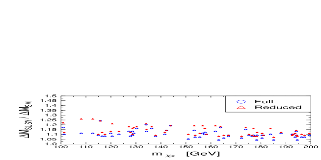
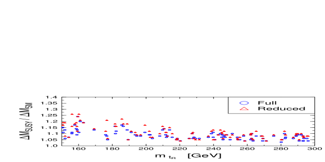
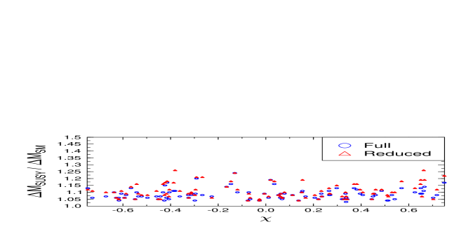
Figure 11: The ratio of the mass–splittings $\Delta M$ within the MSSM and the SM in dependence on $m_{\tilde{t}_{R}}$, $m_{\tilde{\chi}_{2}}$, $\chi$. In all cases we practically decoupled the Higgs boson by setting $M_{H}=1000\,\mbox{\rm GeV}$ and $\tan\!\beta=5$.

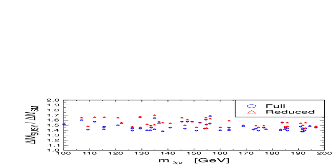
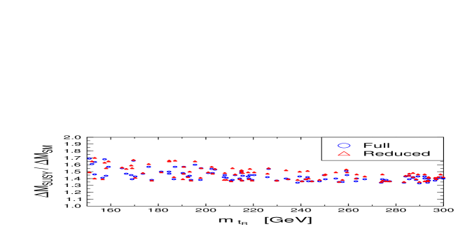
Figure 12: The ratio of the mass–splittings $\Delta M$ within the MSSM and the SM in dependence on $m_{\tilde{t}_{R}}$, $m_{\tilde{\chi}_{2}}$, $\chi$. In all cases we included the Higgs boson by setting $M_{H}=100\,\mbox{\rm GeV}$ and $\tan\!\beta=1.5$.

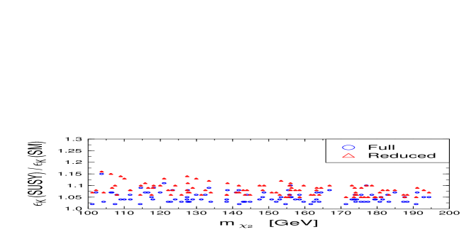
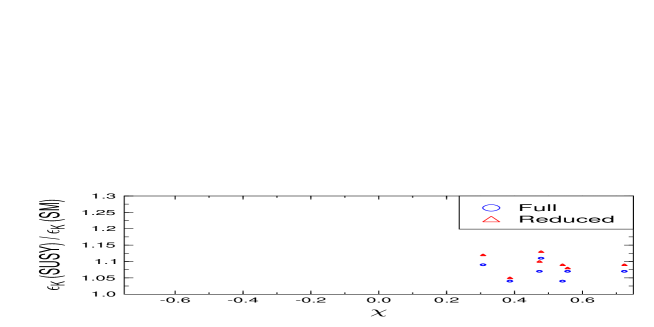
Figure 13: The ratio of $\epsilon_{K}$ within the MSSM and the SM in dependence on $m_{\tilde{t}_{R}}$, $m_{\tilde{\chi}_{2}}$, $\chi$. In all cases we decoupled the Higgs boson by setting $M_{H}=1000\,\mbox{\rm GeV}$ and $\tan\!\beta=5$.

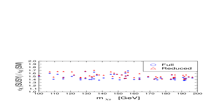
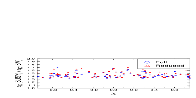
Figure 14: The ratio of $\epsilon_{K}$ within the MSSM and the SM in dependence on $m_{\tilde{t}_{R}}$, $m_{\tilde{\chi}_{2}}$, $\chi$. In all cases we included the Higgs boson by setting $M_{H}=100\,\mbox{\rm GeV}$ and $\tan\!\beta=1.5$.

Obviously – as can be seen in Figs. 11, 12, 13, 14 – the MSSM might have some considerable influence on the observables under consideration and it has clearly the potential to shift the point $(\rho,\eta)$ of the unitarity triangle in the Wolfenstein parametrization. However, an investigation of the effect of gluinos and neutralinos on the NLO–level is still missing and this should be done to have a flavour of the complete picture as predicted by the MSSM. Furthermore, one should investigate the influence of gluino–mediated QCD corrections as accomplished for the decay $b\to s\gamma$ by [31].

Nevertheless we have to remark, that the large range of the Bag–parameters shadows the effect of physics beyond the Standard Model.

Appendix A Inami–Lim Functions

We consider only the very region of low $\tan\!\beta\approx 1$. No scalar operator emerges for the effective Hamiltonian.

A.1 Leading Order Inami–Lim functions

$$S_{WW}(x_{W})=\frac{x_{W}(4-11x_{W}+x_{W}^{2})}{4(1-x_{W})^{2}}-\frac{3x_{W}^{3}\,\log(x_{W})}{2(1-x_{W})^{3}}\,,$$ (41)

$$\tan^{2}\!\!\beta\;S_{HW}(x_{W},x_{H})=$$ (42)

$$-\frac{x_{H}x_{W}}{4}\,\left[\frac{8-2x_{W}}{(1-x_{H})(1-x_{W})}+\frac{(8x_{H}-2x_{W})\,\log(x_{H})}{(1-x_{H})^{2}(x_{H}-x_{W})}\right.$$

$$\;\;\;\;\;\;\;\;\left.-\frac{6\,x_{W}\,\log(x_{W})}{(x_{H}-x_{W})(1-x_{W})^{2}}\right]\,,$$

$$\tan^{4}\!\!\beta\;S_{HH}(x_{W},x_{H})=\frac{x_{H}x_{W}}{4}\,\frac{\left(1-x_{H}^{2}+2\,x_{H}\,\log(x_{H})\right)}{(1-x_{H})^{3}}\,,$$ (43)

$$S_{\chi_{i},\tilde{q}_{a}}(x_{i},y_{a})=$$ (44)

$$\frac{x_{i}+y_{a}}{(x_{i}-y_{a})^{2}}-\frac{2x_{i}y_{a}\log(x_{i})}{(x_{i}-y_{a})^{3}}+\frac{2x_{i}y_{a}\log(y_{a})}{(x_{i}-y_{a})^{3}}\,,$$

$$4S_{\chi_{i,j},\tilde{q}_{a,b}}(x_{i,j},y_{a,b})=$$ (45)

$$\frac{4x_{i}^{2}\log(x_{i})}{(x_{i}-x_{j})(x_{i}-y_{a})(x_{i}-y_{b})}-\frac{4x_{j}^{2}\log(x_{j})}{(x_{i}-x_{j})(x_{j}-y_{a})(x_{j}-y_{b})}+$$

$$\frac{4y_{a}^{2}\log(y_{a})}{(y_{a}-x_{i})(y_{a}-x_{j})(y_{a}-y_{b})}-\frac{4y_{b}^{2}\log(y_{b})}{(y_{b}-x_{i})(y_{b}-x_{j})(y_{a}-y_{b})}\,.$$

A.2 Next–to–Leading Order functions

A.2.1 Standard Model

$$L_{WW}^{(1,8)}(x_{W})=$$ (46)

$$L_{WW,tt}^{(1,8)}(x_{W})-2L_{WW,tu}^{(1,8)}(x_{W})+L_{WW,uu}^{(1,8)}(x_{W})$$

$$+2L_{W\Phi}^{(1,8)}(x_{W})+L_{\Phi\Phi}^{(1,8)}(x_{W})\,\,,$$

$$L^{(1)}_{WW,tt}(x_{W})=$$ (47)

$$\frac{(4\,x_{W}+38\,x_{W}^{2}+6\,x_{W}^{3})\,\log(x_{W})}{(x_{W}-1)^{4}}-\frac{3+28x_{W}+17x_{W}^{2}}{(x_{W}-1)^{3}}$$

$$+\frac{(12\,x_{W}+48\,x_{W}^{2}+12\,x_{W}^{3})\,{\mbox{\rm Li}_{2}}(1-1/x_{W})}{(x_{W}-1)^{4}}$$

$$+\frac{(24x_{W}+48x_{W}^{2})\,{\mbox{\rm Li}_{2}}(1-x_{W})}{(x_{W}-1)^{4}}\,,$$

$$2\,L_{WW,tu}^{(1)}(x_{W})=$$ (48)

$$\frac{2\,(3+13x_{W})}{(x_{W}-1)^{2}}-\frac{2x_{W}\,(5+11x_{W})\,\log(x_{W})}{(x_{W}-1)^{3}}$$

$$-\frac{12x_{W}\,(1+3x_{W})\,{\mbox{\rm Li}_{2}}(1-1/x_{W})}{(x_{W}-1)^{3}}-\frac{24x_{W}\,(1+x_{W}){\mbox{\rm Li}_{2}}(1-x_{W})}{(x_{W}-1)^{3}}\,,$$

$$L^{(1)}_{WW,uu}(x_{W}) = 3\,\,,$$ (49)

$$2\,L_{W\Phi}^{(1)}(x_{W})=$$ (50)

$$\frac{4x_{W}^{2}\,(11+13x_{W})}{(x_{W}-1)^{3}}+\frac{2x_{W}^{2}\,(5+x_{W})(1-9x_{W})\log(x_{W})}{(x_{W}-1)^{4}}$$

$$-\frac{24x_{W}^{2}\,(1+4x_{W}+x_{W}^{2}){\mbox{\rm Li}_{2}}(1-1/x_{W})}{(x_{W}-1)^{4}}$$

$$-\frac{48x_{W}^{2}\,(1+2x_{W}){\mbox{\rm Li}_{2}}(1-x_{W})}{(x_{W}-1)^{4}}\,\,,$$

$$L_{\Phi\Phi}^{(1)}(x_{W})=$$ (51)

$$-\frac{x_{W}^{2}\,(7+52x_{W}-11x_{W}^{2})}{4\,(x_{W}-1)^{3}}+\frac{3x_{W}^{3}\,(4+5x_{W}-x_{W}^{2})\log(x_{W})}{2\,(x_{W}-1)^{4}}$$

$$+\frac{3x_{W}^{3}\,(3+4x_{W}-x_{W}^{2}){\mbox{\rm Li}_{2}}(1-1/x_{W})}{(x_{W}-1)^{4}}+\frac{18x_{W}^{3}\,{\mbox{\rm Li}_{2}}(1-x_{W})}{(x_{W}-1)^{4}}\,\,,$$

$$L^{(8)}_{WW,tt}(x_{W})=$$ (52)

$$\frac{2x_{W}(4-3x_{W})\,\log(x_{W})}{(x_{W}-1)^{3}}-\frac{23-x_{W}}{(x_{W}-1)^{2}}$$

$$+\frac{(8-12x_{W}+12x_{W}^{2})\,{\mbox{\rm Li}_{2}}(1-x_{W})}{(x_{W}-1)^{4}}$$

$$-\frac{(12x_{W}-12x_{W}^{2}-8x_{W}^{3})\,{\mbox{\rm Li}_{2}}(1-1/x_{W})}{(x_{W}-1)^{4}}\,,$$

$$2L^{(8)}_{WW,tu}(x_{W})=$$ (53)

$$\frac{2\,(2-x_{W})\pi^{2}}{3x_{W}}-\frac{(8-5x_{W})\log(x_{W})}{(x_{W}-1)^{2}}-\frac{15}{x_{W}-1}$$

$$-\frac{(6x_{W}+4x_{W}^{2})\,{\mbox{\rm Li}_{2}}(1-1/x_{W})}{x_{W}(x_{W}-1)^{2}}+\frac{(8+12x_{W}-6x_{W}^{2})\,{\mbox{\rm Li}_{2}}(1-x_{W})}{x_{W}(x_{W}-1)^{2}}\,,$$

$$L^{(8)}_{WW,uu}(x_{W}) = -23+\frac{4}{3}\,\pi^{2}\,\,,$$ (54)

$$2\,L_{W\Phi}^{(8)}(x_{W})=$$ (55)

$$\frac{30x_{W}^{2}}{(x_{W}-1)^{2}}+\frac{12x_{W}^{3}\log(x_{W})}{(x_{W}-1)^{3}}-\frac{12x_{W}^{4}\,{\mbox{\rm Li}_{2}}(1-1/x_{W})}{(x_{W}-1)^{4}}$$

$$-\frac{12x_{W}^{2}\,(2\,-x_{W}^{2}){\mbox{\rm Li}_{2}}(1-x_{W})}{(x_{W}-1)^{4}}\,\,.$$

$$L_{\Phi\Phi}^{(8)}(x_{W})=$$ (56)

$$-\frac{11x_{W}^{2}\,(1+x_{W})}{4\,(x_{W}-1)^{2}}+\frac{x_{W}^{3}\,(4\,-3x_{W})\log(x_{W})}{2\,(x_{W}-1)^{3}}$$

$$+\frac{x_{W}^{3}\,(3-3x_{W}+2x_{W}^{2}){\mbox{\rm Li}_{2}}(1-1/x_{W})}{(x_{W}-1)^{4}}$$

$$+\frac{x_{W}^{2}(2+3x_{W}-3x_{W}^{2}){\mbox{\rm Li}_{2}}(1-x_{W})}{(x_{W}-1)^{4}}\,\,,$$

A.2.2 Two Higgs Doublet Model

$$L^{(1,8)}_{\rm THDM}(x_{W},x_{H})=$$ (57)

$$L_{WW}(x_{W})+\frac{1}{\tan^{4}(\beta)}\,HH^{(i)}(x_{H})$$

$$+\frac{2}{\tan^{2}(\beta)}\left[L_{WH}^{(1,8)}(x_{W},x_{H})\,+L_{\Phi H}^{(1,8)}(x_{W},x_{H})\right]\,.$$

$$2\,L_{WH}^{(1)}(x_{W},x_{H})=$$ (58)

$$x_{W}\left[\frac{2x_{H}^{2}(13+3x_{H})\log(x_{H})}{(x_{H}-1)^{3}(x_{H}-x_{W})}\right.-\frac{2x_{H}\,(9+7x_{H}+7x_{W}-23x_{W}x_{H})}{(x_{W}-1)^{2}(x_{H}-1)^{2}}$$

$$\;\;\;\;\;\;\;\;-\frac{2x_{H}^{2}(18-6x_{H}\,-44x_{W}+13x_{H}x_{W}+9x_{H}x_{W}^{2})\log(x_{W})}{(x_{H}-1)^{2}(x_{W}-1)^{3}(x_{H}-x_{W})}$$

$$\;\;\;\;\;\;\;\;+\frac{2x_{H}x_{W}(5-27x_{W}+6x_{W}^{2}+6x_{H}x_{W}^{2})\log(x_{W})}{(x_{H}-1)^{2}(x_{W}-1)^{3}(x_{H}-x_{W})}$$

$$\;\;\;\;\;\;\;\;-\frac{24x_{H}^{2}\,\log(x_{H})\,\log(x_{W})}{(x_{H}-1)^{3}(x_{H}-x_{W})}+\frac{24x_{H}^{2}\,{\mbox{\rm Li}_{2}}(1-1/x_{H})}{(x_{H}-1)^{2}(x_{H}-x_{W})}$$

$$\;\;\;\;\;\;\;\;\left.-\frac{24x_{H}x_{W}\,(1+x_{W})\,{\mbox{\rm Li}_{2}}(1-1/x_{W})}{(x_{W}-1)^{3}(x_{H}-x_{W})}-\frac{48x_{W}x_{H}\,{\mbox{\rm Li}_{2}}(1-x_{W})}{(x_{W}-1)^{3}(x_{H}-x_{W})}\right]\,\,,$$

$$2\,L_{\Phi H}^{(1)}(x_{W},x_{H})=$$ (59)

$$x_{W}^{2}\left[\frac{x_{H}\,(31-15x_{H}-15x_{W}-x_{H}x_{W})}{2\,(x_{H}-1)^{2}\,(x_{W}-1)^{2}}\right.$$

$$\;\;\;\;\;\;\;\;-\frac{x_{H}\,(7+21x_{H}-12x_{H}^{2})\,\log(x_{H})}{2\,(x_{H}-1)^{3}\,(x_{H}-x_{W})}$$

$$\;\;\;\;\;\;\;\;+\frac{x_{H}\,(7-9x_{W}+36x_{W}^{2}-18x_{W}^{3})\,\log(x_{W})}{2(x_{H}-1)^{2}(x_{H}-x_{W})(x_{W}-1)^{3}}$$

$$\;\;\;\;\;\;\;\;+\frac{x_{H}^{2}\,(8-36x_{W}+9x_{W}^{2}+3x_{W}^{3})\log(x_{W})}{(x_{H}-1)^{2}(x_{H}-x_{W})(x_{W}-1)^{3}}$$

$$\;\;\;\;\;\;\;\;-\frac{x_{H}^{3}\,(11-45x_{W}+18x_{W}^{2})\,\log(x_{W})}{2(x_{H}-1)^{2}(x_{H}-x_{W})(x_{W}-1)^{3}}$$

$$\;\;\;\;\;\;\;\;+\frac{6x_{H}\,\log(x_{H})\,\log(x_{W})}{(x_{H}-1)^{3}(x_{H}-x_{W})}-\frac{6x_{H}(1+x_{H}-x_{H}^{2}){\mbox{\rm Li}_{2}}(1-1/x_{H})}{(x_{H}-1)^{2}(x_{H}-x_{W})}$$

$$\;\;\;\;\;\;\;\;+\frac{6x_{H}\,(1+2x_{W}^{2}-x_{W}^{3}){\mbox{\rm Li}_{2}}(1-1/x_{W})}{(x_{H}-x_{W})(x_{W}-1)^{3}}$$

$$\;\;\;\;\;\;\;\;\left.+\frac{12x_{H}\,{\mbox{\rm Li}_{2}}(1-x_{W})}{(x_{H}-x_{W})(x_{W}-1)^{3}}\right]\,\,,$$

$$L_{HH}^{(1)}(x_{W},x_{H})=\frac{x_{W}}{x_{H}}L_{\Phi\Phi}^{(1)}(x_{H})+6\log\frac{x_{H}}{x_{W}}\,\sum_{i=H,W}\frac{x_{i}\partial}{\partial x_{i}}S_{HH}(x_{W},x_{H})\,\,,$$ (60)

$$2\,L_{WH}^{(8)}(x_{W},x_{H})=$$ (61)

$$x_{W}\left[\frac{24x_{H}x_{W}{\mbox{\rm Li}_{2}}(1-x_{W})}{(x_{H}-x_{W})(x_{W}-1)^{2}}\right.$$

$$\;\;\;\;\;\;\;\;+\frac{6x_{H}^{2}(5x_{W}-x_{H}+3x_{W}^{2}x_{H}){\mbox{\rm Li}_{2}}(1-1/x_{W})}{(x_{H}-1)^{2}(x_{H}-x_{W})(x_{W}-1)^{2}x_{W}}$$

$$\;\;\;\;\;\;\;\;+\frac{6x_{H}(2x_{W}^{2}-10x_{H}x_{W}+x_{H}x_{W}^{2}){\mbox{\rm Li}_{2}}(1-1/x_{W})}{(x_{H}-1)^{2}(x_{H}-x_{W})(x_{W}-1)^{2}}$$

$$\;\;\;\;\;\;\;\;+\frac{6x_{H}^{2}(5x_{W}-x_{H}-8x_{W}^{2}+2x_{H}x_{W}^{2}){\mbox{\rm Li}_{2}}(1-x_{H})}{(x_{H}-1)^{2}(x_{H}-x_{W})(x_{W}-1)^{2}x_{W}}$$

$$\;\;\;\;\;\;\;\;+\frac{6(x_{W}^{2}-x_{H}x_{W}+2x_{H}^{2}x_{W}^{2}){\mbox{\rm Li}_{2}}(1-x_{H})}{(x_{H}-1)^{2}(x_{H}-x_{W})(x_{W}-1)^{2}}$$

$$\;\;\;\;\;\;\;\;+\frac{6x_{H}^{2}(-x_{H}+5x_{W}){\mbox{\rm Li}_{2}}(1-1/x_{H})}{(x_{H}-1)^{2}(x_{H}-x_{W})x_{W}}$$

$$\;\;\;\;\;\;\;\;-\frac{6x_{H}^{2}(5x_{W}-x_{H}-8x_{W}^{2}+2x_{H}x_{W}^{2}){\mbox{\rm Li}_{2}}(1-x_{H}/x_{W})}{(x_{H}-1)^{2}(x_{H}-x_{W})(x_{W}-1)^{2}x_{W}}$$

$$\;\;\;\;\;\;\;\;-\frac{6(x_{W}^{2}-x_{H}x_{W}+2x_{H}^{2}x_{W}^{2}){\mbox{\rm Li}_{2}}(1-x_{H}/x_{W})}{(x_{H}-1)^{2}(x_{H}-x_{W})(x_{W}-1)^{2}}$$

$$\;\;\;\;\;\;\;\;-\frac{6x_{H}(1-x_{H}-\log(x_{H}))}{(x_{H}-1)^{2}(x_{W}-1)}+\frac{6x_{H}(2x_{W}-1)\log(x_{W})}{(x_{H}-1)(x_{W}-1)^{2}}$$

$$\;\;\;\;\;\;\;\;+\frac{6x_{H}^{2}(5x_{W}-x_{H}-8x_{W}^{2})\log(x_{H})\log(x_{W})}{(x_{H}-1)^{2}(x_{H}-x_{W})(x_{W}-1)^{2}x_{W}}$$

$$\;\;\;\;\;\;\;\;\left.+\frac{12x_{H}^{2}(x_{H}x_{W}+x_{W}^{2})\log(x_{H})\log(x_{W})}{(x_{H}-1)^{2}(x_{H}-x_{W})(x_{W}-1)^{2}}\right]\,,$$

$$2\,L_{\Phi H}^{(8)}(x_{W},x_{H})=$$ (62)

$$x_{W}^{2}\left[\frac{2x_{H}+2x_{W}-11x_{H}x_{W}}{2\,(x_{H}-1)\,(x_{W}-1)x_{W}}\right.$$

$$\;\;\;\;\;\;\;\;-\frac{(2x_{H}^{2}-7x_{H}x_{W}+2x_{H}^{2}x_{W}+2\,x_{W}^{2}+x_{H}x_{W}^{2})\log(x_{H})}{2\,(x_{H}-1)^{2}\,(x_{H}-x_{W})\,(x_{W}-1)x_{W}}$$

$$\;\;\;\;\;\;\;\;-\frac{x_{H}\,(7-7x_{H}+4x_{W}-6x_{W}^{2})\,\log(x_{W})}{2\,(x_{H}-1)\,(x_{H}-x_{W})\,(x_{W}-1)^{2}}$$

$$\;\;\;\;\;\;\;\;+\frac{(x_{H}^{2}+x_{W}^{2}-3x_{H}^{2}x_{W}^{2})\,\log(x_{W})}{(x_{H}-1)\,(x_{H}-x_{W})\,(x_{W}-1)^{2}x_{W}}$$

$$\;\;\;\;\;\;\;\;-\frac{x_{H}^{2}\,(4-6x_{W}+3x_{H}x_{W})\,\log(x_{H})\,\log(x_{W})}{(x_{H}-1)^{2}\,(x_{H}-x_{W})\,(x_{W}-1)^{2}x_{W}}$$

$$\;\;\;\;\;\;\;\;+\frac{x_{H}\,(x_{H}^{2}-3x_{W}^{2}+6x_{W}^{3}-3x_{W}^{4})\,\log(x_{H})\,\log(x_{W})}{(x_{H}-1)^{2}\,(x_{H}-x_{W})\,(x_{W}-1)^{2}x_{W}^{2}}$$

$$\;\;\;\;\;\;\;\;-\frac{x_{H}\,(3x_{W}^{2}+2x_{H}x_{W}\,(2+x_{W})-x_{H}^{2}\,(1+2\,x_{W}))\,{\mbox{\rm Li}_{2}}(1-1/x_{H})}{(x_{H}-1)^{2}\,(x_{H}-x_{W})x_{W}^{2}}$$

$$\;\;\;\;\;\;\;\;-\frac{(4x_{H}x_{W}-6x_{H}^{2}x_{W}+3x_{H}^{2}x_{W}^{2}-x_{W}^{2}){\mbox{\rm Li}_{2}}(1-x_{H})}{(x_{H}-1)^{2}\,(x_{H}-x_{W})\,(x_{W}-1)^{2}x_{H}}$$

$$\;\;\;\;\;\;\;\;-\frac{(4x_{H}^{2}x_{W}-6x_{H}^{2}x_{W}^{2}-x_{H}^{3}+3x_{H}^{3}x_{W}^{2}){\mbox{\rm Li}_{2}}(1-x_{H})}{(x_{H}-1)^{2}\,(x_{H}-x_{W})\,(x_{W}-1)^{2}x_{W}^{2}}$$

$$\;\;\;\;\;\;\;\;+\frac{2x_{H}^{2}\,(6-x_{W}^{2}-3x_{H}+x_{W}x_{H})\,{\mbox{\rm Li}_{2}}(1-1/x_{W})}{(x_{H}-1)^{2}\,(x_{H}-x_{W})\,(x_{W}-1)^{2}}$$

$$\;\;\;\;\;\;\;\;-\frac{x_{H}\,(3x_{W}^{2}+4x_{H}x_{W}-x_{H}^{2})\,{\mbox{\rm Li}_{2}}(1-1/x_{W})}{(x_{H}-1)^{2}\,(x_{H}-x_{W})\,(x_{W}-1)^{2}x_{W}^{2}}$$

$$\;\;\;\;\;\;\;\;+\frac{(4x_{H}x_{W}-6x_{H}^{2}x_{W}+3x_{H}^{2}x_{W}^{2}-x_{W}^{2}){\mbox{\rm Li}_{2}}(1-x_{H}/x_{W})}{(x_{H}-1)^{2}\,(x_{H}-x_{W})\,(x_{W}-1)^{2}\,x_{H}}$$

$$\;\;\;\;\;\;\;\;+\frac{x_{H}^{2}(4x_{W}-6x_{W}^{2}-x_{H}+3x_{H}x_{W}^{2}){\mbox{\rm Li}_{2}}(1-x_{H}/x_{W})}{(x_{H}-1)^{2}\,(x_{H}-x_{W})\,(x_{W}-1)^{2}\,x_{W}^{2}}$$

$$\;\;\;\;\;\;\;\;\left.-\frac{6x_{H}\,{\mbox{\rm Li}_{2}}(1-x_{W})}{(x_{H}-x_{W})\,(x_{W}-1)^{2}}\right]\,.$$

$$L_{HH}^{(8)}(x_{W},x_{H})=\frac{x_{W}}{x_{H}}L_{\Phi\Phi}^{(8)}(x_{H})+6\log\frac{x_{H}}{x_{W}}\,S_{HH}(x_{W},x_{H})\,\,,$$

A.2.3 MSSM, chargino sector

$$L^{(1)}_{\chi_{i},\tilde{q}_{a}}(y_{a},x_{i})=$$ (63)

$$\frac{19y_{a}^{2}+6y_{a}x_{i}+11x_{i}^{2}}{(x_{i}-y_{a})^{3}}-\frac{2y_{a}(2y_{a}^{2}-11y_{a}x_{i}-9x_{i}^{2})\log(y_{a})}{(x_{i}-y_{a})^{4}}$$

$$-\frac{2x_{i}(4y_{a}^{2}+11y_{a}x_{i}+3x_{i}^{2})\log(x_{i})}{(x_{i}-y_{a})^{4}}++\frac{2y_{a}x_{i}(y_{a}-4x_{i})}{(x_{i}-y_{a})^{4}}(\log^{2}(y_{a})-\log^{2}(x_{i}))$$

$$+\frac{4y_{a}(x_{i}^{2}-x_{i}y_{a}+3y_{a}^{2}){\mbox{\rm Li}_{2}}\left(1-\frac{x_{i}}{y_{a}}\right)}{(x_{i}-y_{a})^{4}}+\frac{4x_{i}y_{a}(4x_{i}-y_{a}){\mbox{\rm Li}_{2}}\left(1-\frac{y_{a}}{x_{i}}\right)}{(x_{i}-y_{a})^{4}}\,,$$

$$L^{(8)}_{\chi_{i},\tilde{q}_{a}}(x_{i},y_{a})=$$ (64)

$$-\frac{7x_{i}+y_{a}}{(x_{i}-y_{a})^{2}}-\frac{2x_{i}(3x_{i}+4y_{a})\log(x_{i})}{(x_{i}-y_{a})^{3}}$$

$$+\frac{2y_{a}(4x_{i}+3y_{a})\log(y_{a})}{(x_{i}-y_{a})^{3}}-\frac{4y_{a}(3x_{i}^{2}-3x_{i}y_{a}-y_{a}^{2})\log(x_{i})\log(y_{a})}{(x_{i}-y_{a})^{4}}$$

$$+\frac{2y_{a}(6x_{i}^{2}-6x_{i}y_{a}-y_{a}^{2})}{(x_{i}-y_{a})^{4}}\log^{2}(x_{i})-\frac{2y_{a}^{3}}{(x_{i}-y_{a})^{4}}\log^{2}(y_{a})$$

$$+\frac{4(x_{i}^{2}+4x_{i}y_{a}+y_{a}^{2})}{(x_{i}-y_{a})^{3}}{\mbox{\rm Li}_{2}}\left(1-\frac{y_{a}}{x_{i}}\right)\,,$$

$$4L^{(1)}_{\chi_{i,j},\tilde{q}_{a,b}}(x_{i,j},y_{a,b})=$$ (65)

$$\left[\frac{-24x_{i}^{2}}{(x_{i}-x_{j})(x_{i}-y_{a})(x_{i}-y_{b})}\;+\;\{i\leftrightarrow j\}\right]$$

$$-\left[\left(\frac{12y_{a}[y_{a}^{2}(y_{b}+2x_{i}+2x_{j})-y_{a}y_{b}(x_{i}+x_{j})]}{(y_{a}-y_{b})(y_{a}-x_{i})^{2}(y_{a}-x_{j})}\right.\right.$$

$$\;\;\;\;\;\;\;\;\left.\left.+\frac{12y_{a}x_{i}x_{j}(y_{b}-4y_{a})}{(y_{a}-y_{b})(y_{a}-x_{i})^{2}(y_{a}-x_{j})^{2}}\right)\log(y_{a})\;+\;\{a\leftrightarrow b\}\right]$$

$$-\left[\left(\frac{4x_{i}[(3y_{a}y_{b}+8x_{i}^{2})(y_{a}+y_{b})-5x_{i}y_{a}y_{b}]}{(x_{i}-x_{j})(x_{i}-y_{a})^{2}(x_{i}-y_{b})^{2}}\right.\right.$$

$$\;\;\;\;\;\;\;\;\left.\left.-\frac{4x_{i}[11x_{i}^{3}-3x_{i}(y_{a}^{2}+y_{b}^{2})]}{(x_{i}-x_{j})(x_{i}-y_{a})^{2}(x_{i}-y_{b})^{2}}\right)\log(x_{i})\;+\;\{i\leftrightarrow j\}\right]$$

$$-\left[\frac{4y_{a}^{2}[4x_{i}x_{j}-3y_{a}(x_{i}+x_{j})+2y_{a}^{2}]}{(y_{a}-y_{b})(y_{a}-x_{i})^{2}(y_{a}-x_{j})^{2}}\log^{2}(y_{a})\;+\;\{a\leftrightarrow b\}\right]$$

$$-\left[\frac{4x_{i}^{2}[3x_{i}^{2}-2x_{i}(y_{a}+y_{b})+y_{a}y_{b}]}{(x_{i}-x_{j})(x_{i}-y_{a})^{2}(x_{i}-y_{b})^{2}}\log^{2}(x_{i})\;+\;\{i\leftrightarrow j\}\right]$$

$$-\left[\frac{4y_{a}(2x_{i}^{2}-3x_{i}y_{a}+3y_{a}^{2})}{(x_{i}-x_{j})(x_{i}-y_{a})^{2}(x_{i}-y_{b})}{\mbox{\rm Li}_{2}}\left(1-\frac{x_{i}}{y_{a}}\right)\;+\;\{i\leftrightarrow j\,,a\leftrightarrow b\}\right]$$

$$-\left[\frac{4x_{i}^{2}(3x_{i}-y_{a})}{(x_{i}-x_{j})(x_{i}-y_{a})^{2}(x_{i}-y_{b})}{\mbox{\rm Li}_{2}}\left(1-\frac{y_{a}}{x_{i}}\right)\;+\;\{i\leftrightarrow j\,,a\leftrightarrow b\}\right]$$

$$-\left[\left(\frac{4y_{b}^{3}[3y_{b}(y_{b}-y_{a}-x_{i}-x_{j})+5y_{a}^{2}+6x_{i}x_{j}]}{(x_{i}-y_{a})(x_{i}-y_{b})(x_{j}-y_{a})(x_{j}-y_{b})(y_{a}-y_{b})^{2}}\right.\right.$$

$$\;\;\;\;\;\;\;\;\left.\left.-\frac{4y_{b}[y_{a}^{2}y_{b}(y_{a}+x_{i}+x_{j})+2x_{i}x_{j}y_{a}(2y_{b}-y_{a})]}{(x_{i}-y_{a})(x_{i}-y_{b})(x_{j}-y_{a})(x_{j}-y_{b})(y_{a}-y_{b})^{2}}\right){\mbox{\rm Li}_{2}}\left(1-\frac{y_{a}}{y_{b}}\right)\right.$$

$$\;\;\;\;\;\;\;\;\;\;\;\;\;\;\;\;\;\;\;\;\;\;\;\;\left.+\vphantom{\frac{|}{|}}\;\{a\leftrightarrow b\}\right]\,,$$

$$4\hbox to0.0pt{$\displaystyle L^{(8)}_{\chi_{i,j},\tilde{q}_{a,b}}(x_{i,j},y_{a,b})=$\hss}$$ (66)

$$\left[\frac{4x_{i}(2x_{i}+x_{j})}{(x_{i}-x_{j})(x_{i}-y_{a})(x_{i}-y_{b})}\log(x_{i})\;+\;\{i\leftrightarrow j\}\right]$$

$$+\left[\frac{4y_{a}(y_{a}+x_{i}+x_{j})}{(y_{a}-y_{b})(y_{a}-x_{i})(y_{a}-x_{j})}\log(y_{a})\;+\;\{a\leftrightarrow b\}\right]$$

$$-\left[\frac{12x_{i}^{2}}{(x_{i}-x_{j})(x_{i}-y_{a})(x_{i}-y_{b})}\log^{2}(x_{i})\;+\;\{i\leftrightarrow j\}\right]$$

$$-\left[\frac{12y_{a}^{2}}{(y_{a}-y_{b})(y_{a}-x_{i})(y_{a}-x_{j})}\log^{2}(y_{a})\;+\;\{a\leftrightarrow b\}\right]$$

$$-\left[\frac{4y_{a}^{2}[3(x_{i}^{2}-y_{a}^{2})-6x_{i}y_{b}+5y_{a}y_{b}]}{(x_{i}-y_{a})^{2}(x_{i}-y_{b})(x_{j}-y_{a})(y_{a}-y_{b})}{\mbox{\rm Li}_{2}}\left(1-\frac{x_{i}}{y_{a}}\right)\right.$$

$$\;\;\;\;\;\;\;\;\;\;\;\;\;\;\;\;\;\;\;\;\;\;\;\;\left.+\vphantom{\frac{|}{|}}\;\{i\leftrightarrow j\,,a\leftrightarrow b\}\right]$$

$$-\left[\left(\frac{4x_{i}^{2}[x_{i}^{2}(2x_{i}-2x_{j}-5y_{a}+y_{b})+3y_{a}^{2}(x_{i}-x_{j})]}{(x_{i}-x_{j})(x_{i}-y_{a})^{2}(x_{i}-y_{b})(x_{j}-y_{a})(y_{a}-y_{b})}\right.\right.$$

$$\;\;\;\;\;\;\;\;\left.\left.+\frac{4x_{i}^{3}[x_{j}(5y_{a}+y_{b})-2y_{a}y_{b}]}{(x_{i}-x_{j})(x_{i}-y_{a})^{2}(x_{i}-y_{b})(x_{j}-y_{a})(y_{a}-y_{b})}\right){\mbox{\rm Li}_{2}}\left(1-\frac{y_{a}}{x_{i}}\right)\right.$$

$$\;\;\;\;\;\;\;\;\;\;\;\;\;\;\;\;\;\;\;\;\;\;\;\;\left.+\vphantom{\frac{|}{|}}\;\{i\leftrightarrow j\,,a\leftrightarrow b\}\right]$$

$$-\left[\left(\frac{4y_{a}^{2}[6y_{a}y_{b}-3(x_{i}+x_{j})(y_{a}+y_{b})]}{(y_{a}-y_{b})(x_{i}-y_{a})(x_{i}-y_{b})(x_{j}-y_{a})(x_{j}-y_{b})}\right.\right.$$

$$\;\;\;\;\;\;\;\;\left.\left.+\frac{4y_{a}^{2}[2x_{i}x_{j}(2y_{a}-3y_{b})+y_{a}y_{b}(x_{i}+x_{j})]}{(y_{a}-y_{b})(x_{i}-y_{a})(x_{i}-y_{b})(x_{j}-y_{a})(x_{j}-y_{b})}\right){\mbox{\rm Li}_{2}}\left(1-\frac{y_{b}}{y_{a}}\right)\right.$$

$$\;\;\;\;\;\;\;\;\;\;\;\;\;\;\;\;\;\;\;\;\;\;\;\;\left.+\vphantom{\frac{|}{|}}\;\{a\leftrightarrow b\}\right]$$

$$-\left[\frac{4x_{i}^{2}[2x_{i}^{2}-3x_{j}^{2}-6(y_{a}y_{b}+x_{i}x_{j})+6(x_{i}+x_{j})(y_{a}+y_{b})]}{(x_{i}-x_{j})(x_{i}-y_{a})(x_{i}-y_{b})(x_{j}-y_{a})(x_{j}-y_{b})}{\mbox{\rm Li}_{2}}\left(1-\frac{x_{j}}{x_{i}}\right)\right.$$

$$\;\;\;\;\;\;\;\;\;\;\;\;\;\;\;\;\;\;\;\;\;\;\;\;\left.+\vphantom{\frac{|}{|}}\;\{i\leftrightarrow j\}\right]\,.$$

Figure 1: Diagrams contributing to $B\overline{B}$–mixing in LO within the SM. The would–be Goldstone bosons $\Phi$ emerging when using the Feynman–t’Hooft gauge are displayed explicitly, crossed diagrams are missing.

Figure 2: Diagrams contributing to $B\overline{B}$–mixing in LO within the THDM. The would–be Goldstone bosons $\Phi$ are subsumed in the labels $W$, crossed diagrams are missing.

Figure 3: Diagrams contributing to $B\overline{B}$–mixing in LO within the MSSM. Only the boxes involving supersymmetric particles are displayed. Note that the neutralinos and gluinos are Majorana–particles. This fact produces graphs like the last one displayed where we have shown explicitly the effect of the Majorana’s character by adding the dots and the direction of the flow with arrows. This feature results in scalar operators.

Table 1: The Feynman–rules employed throughout this article. Note, that only the part proportional to the strong coupling constant enters the four–squark vertex.

Figure 4: Diagrams contributing to the factor $\eta_{2}$ for the QCD–corrections in LO.

Figure 5: Diagrams responsible for explicit QCD–corrections contained in $\eta_{2}$ at NLO within the SM and the THDM.

Figure 6: Diagrams responsible for explicit QCD–corrections contained in $\eta_{2}$ at NLO within the chargino–squark sector of the MSSM.

Figure 7: The product of the CKM–elements $|V_{td}V_{tb}^{\ast}|$ versus $\sqrt{B_{B}f_{B}^{2}}$ for the allowed region of $m_{t}$ within the SM.

Figure 8: The influence of a pure THDM for different values of $M_{H}$ and $\tan\!\beta$. We chose $\sqrt{B_{B}f_{B}^{2}}=0.18\,\mbox{\rm GeV}$, $|V_{td}V_{tb}^{\ast}|=0.007$ and $m_{t}(M_{W})=167\,\mbox{\rm GeV}$.

Figure 9: The ratio of the mass–splittings $\Delta M$ obtained for our “reduced” MSSM and the SM. We assumed a Higgs-mass of $M_{H}=500\,\mbox{\rm GeV}$ and $\tan\!\beta=1.5$.

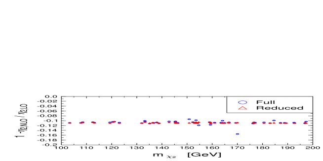
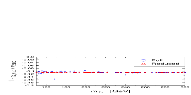
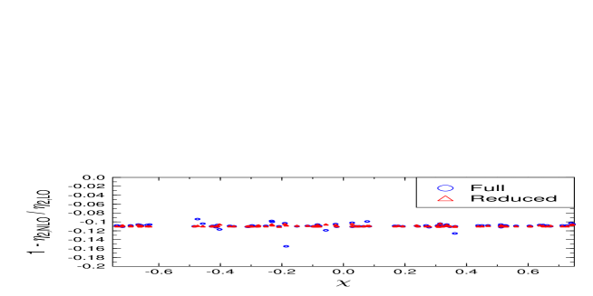
Figure 10: The ratio $\eta_{2LO}/\eta_{2NLO}$ in dependence on $m_{\tilde{t}_{R}}$, $m_{\tilde{\chi}_{2}}$, $\chi$. In all cases we practically decoupled the Higgs boson by setting $M_{H}=1000\,\mbox{\rm GeV}$ and $\tan\!\beta=5$.

Figure 15: The influence of adding THDM and MSSM to the SM on the position of $(\rho,\eta)$. We varied the top–mass within the bounds indicated above as well as the hadronic parameters and chose $M_{H}=200\,\mbox{\rm GeV}$, $\tan\!\beta=1.5$ for the THDM investigations and $M_{H}=500\,\mbox{\rm GeV}$, $\tan\!\beta=5$, $m_{\tilde{t}_{R}}=200\,\mbox{\rm GeV}$ and $m_{\tilde{\chi}_{2}}=120\,\mbox{\rm GeV}$ for the reduced MSSM.

References

• [1] H. E. Haber, G. L. Kane; Phys. Rep. 117 (1985) 75.
• [2] J. F. Gunion, H. E. Haber; Nucl. Phys. B272 (1986) 1.
• [3] J. Wess, J. Bagger; Supersymmetry and Supergravity, Princeton University Press, Princeton, New Jersey (1992).
• [4] H. E. Haber; Introductory Low-Energy Supersymmetry, Proceedings of the 1992 Theoretical Advanced Study Institute in Particle Physics, World Scientific, Singapore (1993) 589.
• [5] L. Maiani, Proc. Summer School of Gif-sur-Yvette, Paris 1980, p. 3;
• [6] M. Veltman, Acta Phys. Pol. B12 (1981) 437;
• [7] E. Witten, NPB 188 (1981) 513.
• [8] M. Drees; An Introduction To Supersymmetry, Lectures given at Inauguration Conference of the Asia Pacific Center for Theoretical Physics (APCTP), Seoul, Korea (1996); hep-ph/9611409.
• [9] S. Dawson; The MSSM and why it works, Lectures given at the 1997 TASI summer school, ”Supersymmetry, Supergravity, and Supercolliders” (1997); hep-ph/9712464.
• [10] S. Bertolini, F. Borzumati, A. Masiero, G. Ridolfi, Nucl. Phys. B353 (1991) 591;
• [11] R. Barbieri, G. F. Giudice, Phys. Lett. B309 (1993) 86;
• [12] N. Oshimo, Nucl. Phys. B404 (1993) 20;
• [13] R. Garisto, J. N. Ng, Phys. Lett. B315 (1993) 372;
• [14] M. A. Diaz, Phys. Lett. B304 (1993) 278;
• [15] Y. Okada, Phys. Lett. B315 (1993) 119;
• [16] F. Borzumati, Z. Phys. C63 (1994) 291;
• [17] P. Nath, R. Arnowitt, Phys. Lett. B336 (1994) 395;
• [18] S. Bertolini, F. Vissani, Z. Phys. C67 (1995) 513;
• [19] J. Lopez et al., Phys. Rev. D51 (1995) 147;
• [20] G. C. Branco, G. C. Cho, Y. Kizukuri, N. Oshimo, Phys. Lett. B337 (1994) 316;
• [21] P. Nath, R. Arnowitt, Phys. Lett. B336 (1994) 395;
• [22] G. C. Branco, W. Grimus, L. Lavoura, Phys. Lett. B380 (1996) 119;
• [23] A. Brignole, F. Feruglio, F. Zwirner, Z. Phys. C71 (1996) 679.
• [24] J. L. Hewett, James D. Wells; Phys. Rev. D55 (1997) 5549.
• [25] J. L. Hewett, T. Takeuchi, S. Thomas; Indirect Probes of New Physics, to appear in Electroweak Symmetry Breaking and Beyond the Standard Model, ed. T. Barklow, S. Dawson, H. Haber, S. Siegrist, World Scientific hep-ph/9603391.
• [26] J. L. Hewett; hep-ph/9803370.
• [27] A. J. Buras, M. Jamin, P. H. Weisz; Nucl. Phys. B347 (1990) 491.
• [28] S. Herrlich, U. Nierste; Phys. Rev. D52 (1995) 6505.
• [29] G. Buchalla, A. J. Buras, M. E. Lautenbacher; Rev. Mod. Phys. 68 (1996) 1125.
• [30] J. Urban, F. Krauss, U. Jentschura, G. Soff; Nucl. Phys. B523 (1998) 40.
• [31] M. Ciuchini, G. Degrassi, P. Gambino, G. F. Giudice; Nucl. Phys. B534 (1998) 3.
• [32] F. Gabbiani, E. Gabrielli, A. Masiero, L. Silvestrini; Nucl. Phys. B477 (1996) 321.
• [33] M. Misiak, S. Pokorski, J. Rosiek; Supersymmetry and FCNC effects, to appear in the Review Volume “Heavy Flavours II”, eds. A. J. Buras and M. Lindner, Advanced Series on Directions in High Energy Physics, World Scientific Publishing Co., Singapore, hep-ph/9703442
• [34] A. Masiero, L. Silvestrini; Two lectures on FCNC and CP violation in Supersymmetry, Lectures given at International School of Subnuclear Physics, 35th Course: Highlights: 50 Years Later, Erice, Italy, 26 Aug - 4 Sep 1997, and given at International School of Physics, ’Enrico Fermi’: Heavy Flavor Physics, hep-ph/9711401;
• [35] Jonathan A. Bagger, Konstantin T. Matchev, Ren-Jie Zhang; Phys. Lett. B412 (1997) 77.
• [36] A. H. Chamseddine, R. Arnowitt, Pran Nath; Phys. Rev.Lett. 49 (1982) 970.
• [37] R. Barbieri, S. Ferrara, C. A. Savoy; Phys. Lett. 119B (1982) 343.
• [38] L. Hall, J. Lykken, S. Weinberg; Phys. Rev. D27 (1983) 2359.
• [39] Pran Nath, R. Arnowitt, A. H. Chamseddine; Nucl. Phys. B227 (1983) 121.
• [40] T. Goto, T. Nihei, Y. Okada; Phys. Rev. D53 (1996) 5233; Erratum-ibid. D54 (1996) 5904.
• [41] W. de Boer; Acta Phys. Polon. B28 (1997) 1395.
• [42] W. de Boer, R. Ehret, A. V. Gladyshev, D. I. Kazakov; hep-ph/9712376.
• [43] J. Erler, D. M. Pierce; hep-ph/9801238.
• [44] J. Rosiek; Phys. Rev. D41 (1990) 3464. Err. in hep-ph/9511250.
• [45] T. Inami, C. N. Lim; Prog. Theor. Phys. 65 (1981) 297.
• [46] F. J. Gilman, M. B. Wise; Phys. Lett. 93B (1980) 129.
• [47] A. J. Buras, P. H. Weisz; Nucl. Phys. B333 (1990) 66.
• [48] W. A. Bardeen, A. J. Buras, D. W. Duke, T. Muta; Phys. Rev. D18 (1978) 3998.
• [49] S. Wolfram; Mathematica: A System for Doing Mathematics by Computer, Addison-Wesley, Reading (1993).
• [50] J. Küblbeck, M. Böhm, A. Denner; Comp. Phys. Comm. 60 (1990) 165
• [51] Particle Data Group; Phys. Rev. D54 (1996) 1.