Mean Field, Instantons and Finite Baryon Density

Abstract

Instantons create a non-local interaction between the quarks, which at finite baryon density leads to the formation of a scalar diquark condensate and color superconductivity. A mean field approach leads to a self-consistent description of the $\langle\bar{q}q\rangle$ and $\langle qq\rangle$ condensates and shows the inevitability of a BCS type instability at the Fermi surface. The role of the rearrangement of the instanton ensemble for the QCD phase transitions is also discussed.

1 Introduction

In the last two decades, instantons were shown to give an explanation of wide range of non-perturbative phenomena - from the binding of the lightest hadrons and the formation of the chiral condensate to the restoration of the chiral symmetry at temperatures of about 150 MeV and the formation of quark gluon-plasma [1]. Although the detailed understanding of the QCD vacuum and of phenomena like the color confinement still remains elusive, lattice studies tend to show that the instantons are the principal non-perturbative configurations in QCD and their role the phenomena mentioned above can be directly observed on the lattice [2]. Unfortunately, one area where the lattice studies are very difficult due to the complex action is the finite baryon density QCD. It seems that the instanton-inspired models are some of the very few methods that work in this area, and recent studies [3, 4, 5] have shown an exciting range of new QCD phases and phenomena like the color superconductivity. One can try to follow faithfully the instanton approach starting directly from the QCD Lagrangian instead of just considering another 4-fermion model interaction. Here we use a mean field treatment of the effective interactions for the case of three colors $N_{c}=3$ and two flavors $N_{f}=2$. We derive the grand canonical potential $\Omega$ at finite baryon chemical potential $\mu$, containing both the chiral $\langle\bar{q}q\rangle$ and the color diquark $\langle qq\rangle$ condensates. We use the exact finite $\mu$ instanton formfactors and show that the gap equations reveal a BCS like instability at the Fermi surface, which leads to a diquark condensation. On the other hand there is a critical coupling for the existence or the chiral condensate, which leads to the restoration of chiral symmetry at high densities.

2 Effective interaction and the finite $\mu$ formfactors

The method of deriving an effective $2N_{f}$-fermion interaction starting from the QCD action was first developed in [6] by D. Diakonov and V. Petrov. It consists of several steps that are sketched below. All momenta and coordinates are Euclidean and we use the Euclidean $\gamma$ matrices. Starting from the QCD partition function,

$$Z=\int{\cal D}\psi{\cal D}\psi^{\dagger}{\cal D}A\exp({S_{QCD}})=\int{\cal D}A\det(\not\!\!D)\exp({S_{gauge}}),$$ (1)

integrate out the fermions to obtain the fermion determinant and separate the low-eigenvalue part from the high-eigenvalue part, by introducing an arbitrary scale

$$\det(\not\!\!D)={\rm Det^{low}}{\rm Det^{high}}.$$ (2)

Consider the classical gauge configuration to consist of an instanton–anti-instanton ensemble. When sufficiently diluted it can be approximated by the sum ansatz

$$A=\sum_{k\in I,\bar{I}}A_{k}+\delta A.$$ (3)

The only collective effects are produced by the zero mode part of the fermion determinant. It consists of

$$T_{I\bar{I}}=\int dtd^{3}{\bf x}\phi_{I}^{\dagger}(x-z_{I})\not\!\partial\phi_{\bar{I}}(x-z_{\bar{I}}),$$ (4)

where $\phi$ are the fermion zero modes. They are known also in the case of finite baryon chemical potential [7]

$$\psi_{0}=-i\frac{\rho}{2\pi\sqrt{\rho^{2}+{x}^{2}}}{e^{\mu\,t}}\sigma_{{\nu}}\left(\partial_{{\nu}}-{\frac{\partial_{{\nu}}(1+{(\rho/x)}^{2})}{1+{(\rho/x)}^{2}}}\right){e^{-\mu\,t}}{1\over x^{2}}\left(\cos(\mu\,r)+{\frac{t}{r}\sin(\mu\,r)}\right)\epsilon_{R},$$ (5)

where $\rho$ is the instanton radius.

Next, reintroduce the fermions, but this time as free fields. Reproduce the zero mode determinant by calculating a Green’s function with $N_{f}(N_{+}+N_{-}+N_{m})$ external legs and using the Wick’s theorem to do the contractions.

$$Z=\int d\psi d\psi^{\dagger}{\exp\{\int d^{4}x\psi^{\dagger}i\not\!\!\partial\psi\}\over N_{+}!N_{-}}\prod_{I=1}^{N_{+}}\theta_{+}\prod_{\bar{I}=1}^{N_{-}}\theta_{-},$$ (6)

where in the two flavor case

$$\theta_{+}=\int dz_{I}d\Omega_{I}\prod_{f=1}^{2}\big{[}\int d^{4}x\psi^{\dagger}_{f}(x)i\not\!\!\partial\phi_{I}(x-z_{I})\int d^{4}y\phi_{I}^{\dagger}(y-z_{I})i\not\!\!\partial\psi_{f}(y)\big{]},$$ (7)

and the integrals are over the collective coordinates of the instantons. To exponentiate the fermion terms, apply inverse Laplace Transformation then go to momentum space and do the integrations over the center coordinates and the orientation angles of the instantons and anti-instantons. The formfactor $\alpha(\omega,k;\mu)$ in the resulting non-local effective Lagrangian is expressed through the Fourier transform of the fermion zero modes. The exact formula depends on the modified Bessel Functions ${\rm I}_{0}(\rho\omega^{\pm}/2)$ and ${\rm K}_{0}(\rho\omega^{\pm}/2)$ and their derivatives, where $\omega^{\pm}=\sqrt{\omega^{+}(k\pm\mu)^{2}}$. The rather lengthy expression shows that the formfactor is centered at the Fermi surface and has a singularity there, but remains finite. Its real and imaginary parts are shown on Fig. 1.

     

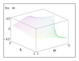
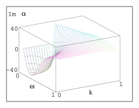
Figure 1: The real and imaginary parts of the formfactor at $\mu=0.5/\rho$. $\omega$ and $k$ are also in units of $1/\rho$.

For the mean field treatment below, it is convenient to write the effective interaction known as ’t Hooft Lagrangian [8] as a sum of the S, T and U channels of the ${\cal T}$ matrix in a tree approximation by doing the appropriate Fierz transforms. The meson channels (S+T) have color singlet and color octet terms, the scalar ones are attractive, while the pseudoscalars are repulsive:

$${\cal L}_{mes} = G\left\{{1\over 8N_{c}^{2}}\left[(\bar{\psi}\tau^{-}\psi)^{2}+(\bar{\psi}\tau^{-}\gamma_{5}\psi)^{2}\right]+{N_{c}-2\over 16N_{c}^{2}(N_{c}^{2}-1)}\left[(\bar{\psi}\tau^{-}\lambda^{a}\psi)^{2}\right.\right.$$ (8)

$$\left.\left.\mbox{}\!\!+(\bar{\psi}\tau^{-}\lambda^{a}\gamma_{5}\psi)^{2}\right]-{1\over 32N_{c}(N_{c}^{2}-1)}(\bar{\psi}\tau^{-}\sigma_{\mu\nu}\lambda^{a}\psi)^{2}\right\}.$$

The diquark channels contains both color antisymmetric ${\bf\bar{3}}$ and symmetric ${\bf 6}$ terms, the scalar and the tensor are attractive:

$${\cal L}_{diq} = G\left\{-{1\over 8N_{c}^{2}(N_{c}-1)}\left[(\psi^{T}C\tau_{2}\lambda_{A}^{a}\psi)(\bar{\psi}\tau_{2}\lambda_{A}^{a}C\bar{\psi}^{T})+(\psi^{T}C\tau_{2}\lambda_{A}^{a}\gamma_{5}\psi)(\bar{\psi}\tau_{2}\lambda_{A}^{a}\gamma_{5}C\bar{\psi}^{T})\right]\right.$$ (9)

$$\left.\mbox{}\!\!+{1\over 16N_{c}^{2}(N_{c}+1)}(\psi^{T}C\tau_{2}\lambda_{S}^{a}\sigma_{\mu\nu}\psi)(\bar{\psi}\tau_{2}\lambda_{S}^{a}\sigma_{\mu\nu}C\bar{\psi}^{T})\right\},$$

where $C$ is the charge conjugation matrix, $\tau_{2}$ is the anti-symmetric Pauli matrix, $\lambda_{A,S}$ are the anti-symmetric (color ${\bf\bar{3}}$) and symmetric (color 6) color generators (normalized in an unconventional way, ${\rm}tr(\lambda^{a}\lambda^{b})=N_{c}\delta^{ab}$, in order to facilitate the comparison between mesons and diquarks). When written in momentum representation, each fermion has a formfactor $\sqrt{\alpha}$ attached to it. The overall coupling constant G comes from the exponentiation of the fermion terms through the inverse Laplace transformation. One can do a saddle point approximation of this integral by varying G and thus relate it to the parameters of the instanton ensemble - total density $n_{inst}$ and average radius $\rho$.

3 Mean field approach

There is a variety of mean field methods, that yield equivalent results. One of the most convenient is the use of a bilocal effective action $\Gamma[G,F,\bar{F}]$ [9, 10, 11], which depends on the propagators $G(x,y)=\langle T\psi(x)\bar{\psi}(y)\rangle,F(x,y)=\langle T\psi(x)\psi^{T}(y)\rangle,$ and $\bar{F}(y,x)=\langle T\bar{\psi}^{T}(x)\bar{\psi}(y)\rangle.$ In momentum representation one obtains:

$$\Gamma[G,F,\bar{F}]=-1/2\rm tr\ln[G(-p)]-1/2\rm tr\ln[G(p)+F(p)(G^{T}(-p))^{-1}\bar{F}(-p)]$$

$$+1/2\rm tr[G_{0}^{-1}(p)G(p)+G_{0}^{-1}(-p)G(-p)-2]+V[G,F,\bar{F}].$$ (10)

Assuming the breakdown both of the chiral and the color symmetry through scalar color singlet $\langle\bar{\psi}\psi\rangle$ and color ${\bf\bar{3}}$ $\langle\psi^{T}C\gamma_{5}\tau_{2}{\vec{\xi}}\cdot{\vec{\lambda}_{A}}\psi\rangle$ condensates, one can write the relevant for the mean field approach terms of the potential $V$ in the zeroth meson-diquark loop approximation

$$V[G,F,\bar{F}]=G{1\over 8N_{c}^{2}}(\rm tr[G_{1}+G_{2}]|\alpha|)^{2}+G{N_{c}-2\over 16N_{c}^{2}(N_{c}^{2}-1)}(\rm tr[\lambda_{8}(G_{1}+G_{2})|\alpha|])^{2}$$

$$+G{1\over 8N_{c}^{2}(N_{c}-1)}\rm tr[C\gamma_{5}\tau_{2}{\vec{\lambda}_{A}}F\alpha(p)]\rm tr[C\gamma_{5}\tau_{2}{\vec{\lambda}_{A}}\bar{F}\alpha(-p)].$$ (11)

The unit vector $\vec{\xi}$ determines the direction of the diquark condensate in the space of $\lambda_{A}$. Without restrictions we can chose it to point towards $\lambda_{2}$. The breakdown of the color symmetry leads to the formation of two different chiral condensates, one involving the quarks of the first two colors, and the second – for the quarks of the third color. Correspondingly, we split the propagator $G=G_{1}+G_{2}$, with $G_{1}$ containing the projector $P$ to the upper left $2\times 2$ square of the SU(3) matrices, while $G_{2}$ containing the projector to the lower right entry. Because both $G_{1}$ and $G_{2}$ mix with the $\lambda_{8}$ matrix, one has to include the color octet interaction term, which contains $\lambda_{8}$. (Please, note again the non-standard normalization of the $\lambda$ matrices.) Varying $\Gamma$ one obtains the Hartree-Fock equations for the propagators. In a picture representation they are shown in Fig. 2.

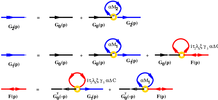
Figure 2: Hartree-Fock equations for the propagators. The effective masses $\tilde{M}_{1},\tilde{M}_{2}$ and the gap $\tilde{\Delta}$ are proportional to the corresponding chiral and color condensates.

The solution of these equations is

$$G_{2} = {-(i\not p^{-}+m_{2})(1-P)\over(p^{-})^{2}+m^{2}},G_{1}={(i\not p^{+}+m_{1})P\over(i\not p^{-}-m_{1})(i\not p^{+}+m_{1})+\Delta^{2}},$$

$$F = {-i\tau_{2}\lambda_{2}C\gamma_{5}\tilde{\Delta}\alpha(-p)\over(i\not p^{+}+m_{1})(i\not p^{-}-m_{1})+\Delta^{2}},$$ (12)

where $\not p^{\pm}=\gamma_{0}(\omega\pm i\mu)+\vec{\gamma}\vec{k}$ and $m_{1,2}=m_{0}+M_{1,2}$, with $m_{0}$ being the current quark mass and $M_{1,2}=\alpha(\omega,k,mu)\tilde{M}_{1,2},\Delta_{1,2}=\alpha(\omega,k,mu)\tilde{\Delta}{1,2}$. Substituting into (10) one obtains the grand canonical potential

$$\Omega(\tilde{M}_{1},\tilde{M}_{2},\tilde{\Delta};\mu)=4\int{d^{4}p\over(2\pi)^{4}}\ln[((\omega_{1}^{+})^{2}+\Delta^{2})((\omega_{1}^{-})^{2}+\Delta^{2})]+2\int{d^{4}p\over(2\pi)^{4}}\ln[(\omega_{2}^{+})^{2}(\omega_{2}^{-})^{2}]$$

$$-16\int{d^{4}p\over(2\pi)^{4}}{m_{1}M_{1}(s_{1}+\Delta^{2}-\mu^{2})+\Delta^{2}(s_{1}+\Delta^{2}+\mu^{2})\over((\omega_{1}^{+})^{2}+\Delta^{2})((\omega_{1}^{-})^{2}+\Delta^{2})}-8\int{d^{4}p\over(2\pi)^{4}}{m_{2}M_{2}(s_{2}-\mu^{2})\over(\omega_{2}^{+})^{2}(\omega_{2}^{-})^{2}}$$

$$+{8\over 9}G\left[\int{d^{4}p|\alpha|\over(2\pi)^{4}}\left({2m_{1}(s_{1}+\Delta^{2}-\mu^{2})\over((\omega_{1}^{+})^{2}+\Delta^{2})((\omega_{1}^{-})^{2}+\Delta^{2})}+{m_{2}(s_{2}-\mu^{2})\over(\omega_{2}^{+})^{2}(\omega_{2}^{-})^{2}}\right)\right]^{2}$$

$$+{1\over 9}G\left[\int{d^{4}p|\alpha|\over(2\pi)^{4}}\left({m_{1}(s_{1}+\Delta^{2}-\mu^{2})\over((\omega_{1}^{+})^{2}+\Delta^{2})((\omega_{1}^{-})^{2}+\Delta^{2})}-{m_{2}(s_{2}-\mu^{2})\over(\omega_{2}^{+})^{2}(\omega_{2}^{-})^{2}}\right)\right]^{2}$$

$$+{2\over 3}G\left[\int{d^{4}p|\alpha|\over(2\pi)^{4}}{\Delta(s_{1}+\Delta^{2}+\mu^{2})\over((\omega_{1}^{+})^{2}+\Delta^{2})((\omega_{1}^{-})^{2}+\Delta^{2})}\right]^{2},$$ (13)

where $(\omega_{1,2}^{\pm})^{2}=\omega^{2}+(\sqrt{k^{2}+m_{1,2}^{2}}\pm\mu)^{2}$, $s_{1,2}=\omega^{2}+k^{2}+m_{1,2}^{2}$. By differentiating with respect to $\tilde{M}_{1},\tilde{M}_{2}$ and $\tilde{\Delta}$ one can obtain a system of coupled gap equations, which can be solved numerically for each value of $\mu$. An easier approach for studying the phase diagram of the system is to plot $\Omega$ as a function of two of the parameters for different values of $\mu$ and a fixed third parameter. The minima will correspond to the different possible phases and the phase transitions correspond to two minima having an equal value (first order), or joining together (second order). But even without a computer, one can study the limiting cases – pure chiral condensate ($\tilde{M}_{1}=\tilde{M}_{2},\tilde{\Delta}=0$), or pure diquark condensate ($\tilde{M}_{1}=\tilde{M}_{2}=0$). The corresponding gap equations have the following form:

$$1 = {1\over 12}G\int{d^{4}p\over(2\pi)^{4}}{(s_{1}+\Delta^{2}+\mu^{2})|\alpha|^{2}\over((\omega_{1}^{+})^{2}+\Delta^{2})((\omega_{1}^{-})^{2}+\Delta^{2})},$$ (14)

$$1 = {2\over 3}G\int{d^{4}p\over(2\pi)^{4}}{(s_{1}-\mu^{2})|\alpha|^{2}\over(s_{1}-\mu^{2})^{2}+4\mu^{2}\omega^{2}},$$ (15)

The formfactor $|\alpha|$, which enters in $M_{1},M_{2},\Delta$, although having a cusp at $k=\mu$ is also continuous, so that for the qualitative picture one can substitute it with a sharp cutoff around the Fermi surface. If we remove the gap $\tilde{\Delta}$ the first equation develops a logarithmic divergence of the BCS type and can not be satisfied for any G:

$$1={1\over 96\pi^{2}}GF_{1}\left[\int_{\mu-\epsilon}^{\mu+\epsilon}{k^{2}dk\over k+\mu}+\int_{\mu}^{\mu+\epsilon}{k^{2}dk\over k-\mu}+\int_{\mu-\epsilon}^{\mu}{k^{2}dk\over\mu-k}\right].$$ (16)

The last two terms, which are divergent correspond to quarks and holes close to the Fermi surface $k=\mu$. The second equation, however, is of Nambu type

$$1={1\over 6\pi^{2}}GF_{2}\int_{(\mu^{2}-m^{2})^{1/2}}^{mu+\epsilon}{k^{2}dk\over\sqrt{k^{2}+m^{2}}}$$ (17)

and needs a minimal critical coupling for a solution to exist even at finite $\mu$. Note also that the Fermi momentum $k_{F}=\sqrt{\mu^{2}-m^{2}}$. Similar conclusions were reached in [3] using a different method and ad-hoc formfactors.

4 Phase Transitions

Although in the picture drawn so far there can be phase transitions, they may be very dependent on the particular scenario, e.g. in [3] the chiral restoration transition is due mainly to the formfactor which is centered not at $k=\mu$, but at $k=0$, so that at sufficiently large chemical potential, it cuts off effectively the interaction. Another possibility is the Debye screening of the instantons in the plasma phase, which also leads to decrease in the effective four-fermion coupling. Studies of the finite temperature chiral restoration transition [12, 13], has shown the importance of the correlations in the instanton ensemble, which grow with $T$. One can take into account these correlations in the mean field approach by considering the tightly bound and polarized instanton – anti-instanton pairs as new objects called molecules, which form a new component. The phase transition is characterized by complete pairing of all instantons into molecules. The role of the molecules is to deplete the random component, which is responsible for the collectivization of the zero modes and it also provides additional four-fermion interactions.

At finite chemical potential, two mechanisms for suppressing $\langle\bar{\psi}\psi\rangle$ may exist: the depletion of the random component by the molecules, and the competition from $\langle\psi\psi\rangle$ - i.e. instantons previously engaged in the infinite “vacuum quark clusters” (the collectivized zero modes) become engaged in the “matter diquark chains”.

If $\mu>>m_{s}$, we should consider the $s$ quark as a light one and study the phase diagram as a function of its mass too. As recent papers has shown [4]the phase structure in the $N_{f}=3$ case is richer and more exotic. There is the possibility of many new condensates, and patterns of symmetry breaking, i.e. ${SU(3)_{c}}\times{SU(3)_{f}}\to SU(3)_{d}$. The color superconductivity is complete, because there is a gap for all quarks. In this case the instantons can not form alone a diquark condensate, but the molecules can. Their contribution to the diquark binding may be not a correction, but the main one.

5 Conclusion

The mean field approach to the instanton induced quark interaction has proved itself as a reliable method to study the richness of QCD phenomena at finite baryon density, a situation in which very few other methods seem to work. It has shown that the expectations of a BCS type of superconductivity transition were correct, and simultaneously they show how the chiral symmetry is restored. However, if one wants to make this approach more realistic, he should take into account the correlations and the restructuring of the instanton ensemble, something that has been shown to play the key role in the finite temperature phase transition.

6 Acknowledgements

I would like to thank my collaborators Edward Shuryak, Ralf Rapp and Thomas Schäfer for the useful discussions. I also want to thank D. Diakonov for the healthy criticism and the interesting discussions.

References

- [1] For a review see T. Schäfer and E. Shuryak, Rev. Mod. Phys. 70, 323-426 (1998).
- [2] M. C. Chu, J. M. Grandy, S. Huang and J. W. Negele, Phys. Rev. Lett. 70, 225 (1993); M. C. Chu and S. Huang, Phys. Rev. D45, 7 (1992). M. C. Chu, J. M. Grandy, S. Huang, J. W. Negele, Phys. Rev. D49, 6039 (1994). C. Michael, P. S. Spencer, Nucl. Phys. (Proc. Suppl.) B42, 261 (1995); Phys. Rev. D50, 7570 (1995).
- [3] M. Alford, K. Rajagopal, F. Wilczek Phys. Lett. B422, 247 (1998), e-Print Archive: hep-ph/9711395.
- [4] J. Berges, K. Rajagopal Preprint MIT-CTP-2725, Apr 1998. e-Print Archive: hep-ph/9804233
- [5] R. Rapp, T. Schäfer, E. Shuryak, M. Velkovsky e-Print Archive: hep-ph/9711396, to appear in Phys. Rev. Lett.
- [6] D. I. Diakonov, V. Yu. Petrov ”Spontaneous breaking of chiral symmetry in the instanton vacuum”, preprint LNPI-1153 (1986), published in: Hadron matter under extreme conditions, Kiev (1986) p. 192. D. I. Diakonov, V. Yu. Petrov Sov.Phys.Jetp 62, 204 ( 1985) (Zh. Eksp. Teor. Fiz. 89, 361 (1985)) Nucl. Phys. B272, 457 (1986).
- [7] A.A. Abrikosov, Jr., Yad. Fiz. (Sov. J. of Nucl. Phys.) 37, 772 (1983).
- [8] G. ’t Hooft Phys. Rev. D14, 3432(1976).
- [9] J. M. Cornwall, R. Jackiw and E. Tombolis, Phys. Rev. D10, 2428 (1974).
- [10] M. Lutz, J. Praschifka, Int. Jour. Mod. Phys A8, 277 (1993).
- [11] D. I. Diakonov, M. Lutz, Preprint ECT*/Dec/95-003, e-Print Archive: hep-ph/9512385.
- [12] T. Schäfer and E. Shuryak, Phys. Rev. D53, 6522 (1996).
- [13] M. Velkovsky, E. Shuryak Phys. Rev. D56, 2766 (1997).