Dimensionally Regularized Study of Nonperturbative
Quenched QED

Abstract

We study the dimensionally regularized fermion propagator Dyson-Schwinger equation in quenched nonperturbative QED in an arbitrary covariant gauge using the Curtis-Pennington vertex and perform nonperturbative renormalization numerically. The nonperturbative fermion propagator is solved in $D\equiv 4-2\epsilon<4$ dimensional Euclidean space for a large number of values of $\epsilon$ for two values of the coupling, $\alpha=0.6$ and $\alpha=1.5$. Results for $D=4$ are then obtained by extrapolation to $\epsilon\to 0$. We compare these results against previous studies employing a modified ultraviolet cut-off regularization and find agreement to within the numerical precision of the present calculations.

1 Introduction

The Dyson-Schwinger equations (DSE) are an infinite tower of integral equations that self-consistently relate the Green’s functions of a field theory. They provide an alternative to lattice gauge theory [1] for investigating nonperturbative phenomena such as dynamical chiral symmetry breaking and dynamical mass generation. The advantage of such a continuum formulation is that it is at times possible to obtain analytical insights, there is no limit to the momentum range that can be studied and one is able to compare different regularization schemes. The disadvantage is that the tower has to be truncated to those equations involving Green’s functions with relatively few external legs: consequently some of the Green’s functions appearing in the remaining equations are no longer determined self-consistently by the DSE’s and we must make an educated guess (Ansatz) regarding their form.

As an example, quantum electrodynamics (QED) in four dimensions in the DSE formalism [2, 3, 4] admits a dynamical mass above a certain critical coupling. The coupled integral equations determining the photon and fermion propagators are completely closed once the photon-fermion proper vertex is specified. The quenched approximation, in which the photon propagator is bare and the coupling does not run with momentum, reduces the study of these coupled equations to that of the fermion propagator: for computational reasons it is almost universally used at present. The vertex Ansatz is constrained by the need to respect the discrete symmetries and the Ward-Takahashi identities [5] (WTI), have no artificial kinematic singularities, satisfy the requirements of perturbative multiplicative renormalizability (MR), and agree with perturbation theory in the weak coupling limit. Furthermore the gauge dependence of the resulting fermion propagator should be consistent with the Landau-Khalatnikov transformation [6]. Ultimately, observables like the critical coupling should be verified to be gauge-independent, once the effect of the regulator is removed.

A number of discussions of the choice of proper vertex in quenched QED can be found in the literature, e.g., Refs. [7, 8, 9, 10, 11, 12, 13, 14, 15]. Here we concentrate on the Curtis-Pennington (CP) vertex, which satisfies both the WTI and the constraints of multiplicative renormalizability. With a bare vertex (which breaks both gauge invariance and MR) the critical coupling of quenched QED differs by approximately 50% when calculated in the Feynman and Landau gauge. This should be compared to a difference of less than 2% if this quantity is calculated with the Curtis-Pennington vertex [11, 16]. Similar results are obtained in [18]. These calculations used a form of the ultraviolet (UV) regulated DSE with a gauge covariance correction, where an obvious gauge covariance violating term arising from the cut-off was omitted.

Clearly, the gauge dependence of the critical coupling is decreased, but not eliminated, through the use of a photon-fermion proper vertex which satisfies the WTI. The question arises whether the remaining slight gauge dependence in the critical coupling is primarily due to limitations of the vertex itself or whether it is due to the use of a UV cut-off regulator in these calculations. Bashir and Pennington [13, 14] have pursued the first of these alternatives and have obtained, within a cut-off regularized theory, further restrictions on the transverse part of the vertex which ensure by construction that the critical coupling indeed becomes strictly gauge independent. It is not clear that adjusting the vertex to remove an unwanted gauge-dependence is the most appropriate procedure when using a gauge-invariance (and Poincaré-invariance) violating regularization scheme.

We explore the second alternative by studying renormalized quenched QED numerically using the CP vertex and dimensional regularization [20] where gauge invariance is explicitly maintained. To our knowledge this is the first complete nonperturbative demonstration of dimensional regularization and renormalization, and follows procedures first developed using the DSE for a UV cutoff regulator in Refs. [17, 18, 19]. The resulting nonlinear integral equation for the fermion propagator is solved numerically in $D=4-2\epsilon<4$ Euclidean dimensional space. Successive calculations with decreasing $\epsilon$ are then extrapolated to $\epsilon=0$ and compared with the corresponding (modified and unmodified) UV cutoff results.

2 Formalism

We summarize the implementation of nonperturbative renormalization using dimensional regularization within the context of numerical DSE studies, adopting a notation similar to that used in Refs. [17, 18, 19]. The formalism is presented in Minkowski space and the Wick rotation into Euclidean space can then be performed once the equations to be solved have been written down. Note we use dimensional regularization in conjunction with off-shell renormalization, rather than using the $MS$ or $\overline{MS}$ renormalization schemes, which can only be defined in a perturbative context.

The renormalized inverse fermion propagator is defined through

$$S^{-1}(\mu;p)=A(\mu;p^{2})\not\!p-B(\mu;p^{2}) = Z_{2}(\mu,\epsilon)[\not\!p-m_{0}(\epsilon)]-\Sigma^{\prime}(\mu,\epsilon;p)$$ (1)

$$= \not\!p-m(\mu)-\widetilde{\Sigma}(\mu;p)\;\;\;,$$

where $\mu$ is the chosen renormalization scale, $m(\mu)$ is the value of the renormalized mass at $p^{2}=\mu^{2}$, $m_{0}(\epsilon)$ is the bare mass and $Z_{2}(\mu,\epsilon)$ is the wavefunction renormalization constant. Due to the WTI for the fermion-photon proper vertex, we have for the vertex renormalization constant $Z_{1}(\mu,\epsilon)=Z_{2}(\mu,\epsilon)$. The renormalized and unrenormalized fermion self-energies are denoted as $\widetilde{\Sigma}(\mu;p)$ and $\Sigma^{\prime}(\mu,\epsilon;p)$ respectively. These can be expressed in terms of Dirac and scalar pieces, where for example

$$\Sigma^{\prime}(\mu,\epsilon;p)=\Sigma^{\prime}_{d}(\mu,\epsilon;p^{2})\not\!p+\Sigma^{\prime}_{s}(\mu,\epsilon;p^{2})\;\;\;,$$ (2)

and similarly for $\widetilde{\Sigma}(\mu;p)$. In the interests of notational brevity we do not explicitly indicate the dependence on $\epsilon$ of the renormalized quantities $A(\mu;p^{2})$, $B(\mu;p^{2})$ and $\widetilde{\Sigma}(\mu;p)$, since for these and other renormalized quantities we are always interested in their $\epsilon\to 0$ limit. The renormalized mass function $M(p^{2})\equiv B(\mu;p^{2})/A(\mu;p^{2})$ is renormalization point independent, which follows straightforwardly from multiplicative renormalizability [18].

The renormalization point boundary condition

$$\left.S^{-1}(\mu;p)\right|_{p^{2}=\mu^{2}}=\not\!p-m(\mu)\>$$ (3)

implies that $A(\mu;\mu^{2})\equiv 1$ and $m(\mu)\equiv M(\mu^{2})$ and yields the following relations between renormalized and unrenormalized self-energies

$$\widetilde{\Sigma}_{d,s}(\mu;p^{2})=\Sigma^{\prime}_{d,s}(\mu,\epsilon;p^{2})-\Sigma^{\prime}_{d,s}(\mu,\epsilon;\mu^{2})\;\;\;.$$ (4)

Also, the wavefunction renormalization is given by

$$Z_{2}(\mu,\epsilon)=1+\Sigma^{\prime}_{d}(\mu,\epsilon;\mu^{2})$$ (5)

and the bare mass $m_{0}(\epsilon)$ is linked to the renormalized mass $m(\mu)$ through

$$m_{0}(\epsilon)=\left[m(\mu)-\Sigma^{\prime}_{s}(\mu,\epsilon;\mu^{2})\right]/Z_{2}(\mu,\epsilon)\;\;\;.$$ (6)

It also follows from MR that under a renormalization point transformation $\mu\to\mu^{\prime}$, $m(\mu^{\prime})=M({\mu^{\prime}}^{2})$ and $Z_{2}(\mu^{\prime},\epsilon)=A(\mu^{\prime};\mu^{2})\,Z_{2}(\mu,\epsilon)$ as discussed in [18].

The unrenormalized self-energy is given by the integral

$$\Sigma^{\prime}(\mu,\epsilon;p)=iZ_{1}(\mu,\epsilon)[e(\mu)\nu^{\epsilon}]^{2}\int\frac{d^{D}k}{(2\pi)^{D}}\gamma^{\lambda}{S}(\mu;k){\Gamma}^{\nu}(\mu;k,p){D}_{\lambda\nu}(\mu;p-k)\>,$$ (7)

where $\nu$ is an arbitrary mass scale introduced in $D$ dimensions so that the renormalized coupling $e(\mu)$ remains dimensionless. Since we are here working in the quenched approximation we have $Z_{3}(\mu,\epsilon)=1$, $e_{0}\equiv e(\mu)$, and the renormalized photon propagator ${D}^{\mu\nu}(\mu;q)$ is equal to the bare photon propagator

$$D^{\mu\nu}(q)=\left(-g^{\mu\nu}+\frac{q^{\mu}q^{\nu}}{q^{2}}-\xi\frac{q^{\mu}q^{\nu}}{q^{2}}\right)\frac{1}{q^{2}}\>$$ (8)

with $\xi$ being the covariant gauge parameter. Finally, ${\Gamma}^{\nu}(\mu;k,p)$ is the renormalized photon-fermion vertex for which we use the CP Ansatz, namely ($q\equiv k-p$)

$$\Gamma^{\mu}(\mu;k,p)=\Gamma_{\rm BC}^{\mu}(\mu;k,p)+\tau_{6}(\mu;k^{2},p^{2},q^{2})\left[\gamma^{\mu}(p^{2}-k^{2})+(p+k)^{\mu}{\not\!q}\right]\>,$$ (9)

where $\Gamma_{\rm BC}$ is the usual Ball-Chiu part of the vertex which saturates the Ward-Takahashi identity [7]

$$\Gamma^{\mu}_{\rm BC}(\mu;k,p) = \frac{1}{2}[A(\mu;k^{2})+A(\mu;p^{2})]\gamma^{\mu}$$

$$+\frac{(k+p)^{\mu}}{k^{2}-p^{2}}\left\{[A(\mu;k^{2})-A(\mu;p^{2})]\frac{{\not\!k}+{\not\!p}}{2}-[B(\mu;k^{2})-B(\mu;p^{2})]\right\}$$

and the coefficient function $\tau_{6}$ is that chosen by Curtis and Pennington, i.e.,

$$\tau_{6}(\mu;k^{2},p^{2},q^{2})=-\frac{1}{2}[A(\mu;k^{2})-A(\mu;p^{2})]/d(k,p)\>,$$ (11)

where

$$d(k,p)=\frac{(k^{2}-p^{2})^{2}+[M^{2}(k^{2})+M^{2}(p^{2})]^{2}}{k^{2}+p^{2}}\>.$$ (12)

The unrenormalized scalar and Dirac self–energies are extracted out of the DSE, Eq. (7), by taking $\frac{1}{4}{\rm Tr}$ of this equation, multiplied by 1 and $\not\!p/p^{2}$, respectively. Note that we use the following conventions [21] for the Dirac algebra:

$$g^{\mu}{}_{\mu}\>=D\hskip 28.45274pt \Rightarrow \hskip 28.45274pt\gamma^{\mu}\gamma_{\mu}=D,\quad\gamma^{\mu}\gamma^{\nu}\gamma_{\mu}=(2-D)\gamma^{\nu}$$

$${\rm Tr}[{\bf 1}]\>=\>4\hskip 28.45274pt \Rightarrow \hskip 28.45274pt{\rm Tr}\left[\gamma^{\mu}\gamma^{\nu}\right]=4g^{\mu\nu}.$$

The integrands appearing in Eq. (7) only depend on the magnitude of the internal fermion’s momentum $k^{2}$ as well as the angle $\theta$ between the fermion and photon momentum. Hence the D-dimensional integrals reduce to 2-dimensional ones, i.e.,

$$\int d^{D}k\,f(k^{2},p^{2},k\cdot p)=\int d\Omega^{D-1}\times\int_{0}^{\infty}dk\,k^{D-1}\int_{0}^{\pi}d\theta\>\sin^{D-2}\theta\>f(k^{2},p^{2},k\cdot p)$$ (13)

where

$$\int d\Omega^{D}=\frac{2\pi^{D/2}}{\Gamma(D/2)}$$ (14)

is the surface area of a D-dimensional sphere. Furthermore, it is possible to express all the angular integrals in terms of a single hypergeometric function so that it is only necessary to do the momentum integral numerically, solving the renormalized fermion DSE by iteration. Note that the momentum integration extends to infinity, necessitating a change in integration variables. The infinite range of the integration also requires an extrapolation of $A(\mu;p^{2})$ and $B(\mu;p^{2})$ above the highest gridpoint. We check insensitivity to this extrapolation by comparing results obtained with a number of different extrapolation prescriptions. In addition, we use grids which extend some 20-30 orders of magnitude beyond what is usually used in cut-off studies. We have verified the effect of the extrapolation to infinity is well-controlled.

3 Results

We present solutions for the DSE for two values of the coupling $\alpha=e_{0}^{2}/4\pi$, namely $\alpha=0.6$ and $\alpha=1.5$, chosen to correspond to couplings respectively well below and above the critical coupling found in previous UV cut-off based studies. Note that all results are quoted in terms of dimensionless units, i.e., all mass and momentum scales can be simultaneoulsy multiplied by any desired mass scale.

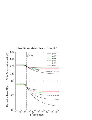
(a)

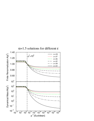
(b)

Figure 1: The finite renormalization $A(p^{2})$ and mass function $M(p^{2})$ for various choices of the regulator parameter $\epsilon$. Figure 1(a) has coupling $\alpha=0.6$ and 1(b) $\alpha=1.5$, with gauge parameter $\xi=0.25$, renormalization point $\mu^{2}=10^{8}$, renormalized mass $m(\mu)=400$ and scale $\nu=1$. In the low $p^{2}$ region the smallest $\epsilon$ has the largest value of $M(p^{2})$.

Fig. 1 show a family of solutions with the regulator parameter $\epsilon$ decreased from $0.08$ to $0.03$ for the two values of the coupling. We see that the mass function increases in strength in the infrared and tails off faster in the ultraviolet as $\epsilon$ is reduced or $\alpha$ is increased. Furthermore, it is important to note the strong dependence on $\epsilon$, even though this parameter is already rather small. As one would expect, the ultraviolet is most sensitive to this regulator, however even in the infrared there is considerable dependence due to the intrinsic coupling between these regions by the renormalization procedure. This strong dependence on $\epsilon$ should be contrasted with the situation in cut-off based studies where it was observed that already at rather modest cut-offs ($\Lambda^{2}\approx 10^{10}$) the renormalized functions $A$ and $M$ had reached their asymptotic limits.

Currently it is not possible to decrease $\epsilon$ significantly below the values shown in Fig. 1 due to numerical limitations. In order to extract the values of $A$ and $M$ in four dimensions we extrapolate to $\epsilon=0$, which introduces an added uncertainty in the final result. However it is possible to estimate this uncertainty by using the fact that in the limit $\epsilon\rightarrow 0$ the renormalized quantities should become independent of the arbitrary scale $\nu$, introduced to keep the coupling $\alpha$ dimensionless in $D$ dimensions.

(a)

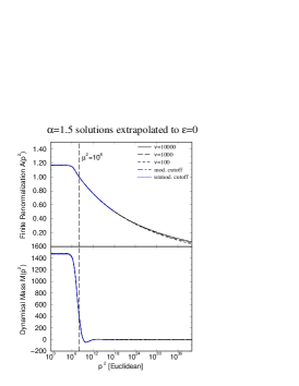
(b)

Figure 2: (a) shows the finite renormalization $A(p^{2})$ and mass function $M(p^{2})$ evaluated at $p^{2}=1$ for various values of the regulator parameter $\epsilon$ and extrapolated to $\epsilon=0$ by fitting a polynomial cubic in $\epsilon$. Shown are five scales $\nu=1$, $10$, $100$, $1000$ and $10000$. All other parameters are those of Fig. 1. The different scales coincide at $\epsilon=0$ to an accuracy of approximately $0.2\%$. (b) shows the finite renormalization $A(p^{2})$ and mass function $M(p^{2})$ extrapolated to $\epsilon=0$ at each momentum point for the three scales $\nu=100$, $1000$ and $10000$. Also shown are results obtained using a modified and unmodified UV cutoff. The modified UV cutoff and extrapolated results are indistinguishable in these plots, and differ from those of the unmodified UV cutoff in the IR.

In Fig. 2a we show $A(p^{2})$ and $M(p^{2})$ evaluated with $\alpha=e_{0}^{2}/4\pi=1.5$ in the infrared (at $p^{2}=1$) as a function of $\epsilon$ for a range of values of $\nu$. The results at $\epsilon=0$ are extracted from cubic polynomial fits in $\epsilon$. The agreement between the different curves at $\epsilon=0$ is excellent, being of the order of $0.2\%$. In Fig. 2b we show the results for $\nu=100$, $1000$ and $10000$ extrapolated to $\epsilon=0$ as a function of momentum for $\alpha=1.5$. Again the agreement is very good for a wide range of $p^{2}$ and $\nu$. Only in the ultraviolet region (above say $p^{2}=10^{12}$) are differences between the curves discernible. The discrepancies for $\nu=1$ and $10$ cases were somewhat greater in the UV, presumably reflecting greater non-linearity in the fits for these cases that is manifest at $p^{2}=0$ in Fig. 2a. This is supported by the observation that these lower-scale cases were more sensitive to changing the order of the polynomial the higher-scale cases. Also shown in Fig. 2b are the corresponding UV cutoff results, both with and without a modification which used a gauge-covariance fix to remove an obvious part of the gauge dependence induced by the cutoff [18]. The modified UV cutoff curve is indistinguishable from the scaled dimensionally regularized ones, while the unmodified UV cutoff curve clearly deviates from the others in the IR. It should also be noted that the oscillatory behaviour in the mass function first noticed in [17] is reproduced in this work.

4 Conclusions and Outlook

We have reported the first detailed study of the numerical renormalization of the fermion Dyson-Schwinger equation of QED through the use of a dimensional regulator rather than a gauge invariance-violating UV cut-off. The initial results are encouraging. Firstly, we have explicitly demonstrated that the approach works and is independent of the intermediate dimensional regularization scale as expected. Secondly, the previously obtained modified UV cut-off results are reproduced with considerable precision.

A significant practical difference between the dimensionally and UV cut-off regularized approaches is that in the former it is currently necessary to perform an explicit extrapolation to $\epsilon=0$ whereas in the latter for a sufficiently large choice of UV cut-off the results became independent of the cut-off. We are presently investigating whether it is numerically possible to extend the studies to smaller values of $\epsilon$ in order to improve the precision of the $\epsilon\to 0$ extrapolation. In the meantime, the extrapolation to $\epsilon=0$ appears to be well under control, at least for values of the fermion momentum away from the ultraviolet region.

Having demonstrated the numerical procedure of renormalization using dimensional regularization, we plan to study chiral symmetry breaking and in particular hope to extract the critical coupling as a function of the gauge parameter, and to shed further light on the nature of the chiral limit discussed in [19]. Results of this work will be presented elsewhere. The eventual aim is to extend this treatment to the case of unquenched QED.

References

References

- [1] H.J. Rothe, Lattice Gauge Theories: an Introduction, (World Scientific, Singapore, 1992).
- [2] C.D. Roberts and A.G. Williams, Dyson-Schwinger Equations and their Application to Hadronic Physics, in Progress in Particle and Nuclear Physics, Vol. 33 (Pergamon Press, Oxford, 1994), p. 477.
- [3] V. A. Miranskii, Dynamical Symmetry Breaking in Quantum Field Theories, (World Scientific, Singapore, 1993).
- [4] P. I. Fomin, V. P. Gusynin, V. A. Miransky and Yu. A. Sitenko, Riv. Nuovo Cim. 6, 1 (1983).
- [5] J.C. Ward, Phys. Rev. 78, 124 (1950); Y. Takahashi, Nuovo Cimento 6, 370 (1957).
- [6] L. D. Landau and I. M. Khalatnikov, Sov. Phys. JETP 2, 69 (1956) [translation of Zhur. Eksptl. i Teoret. Fiz. 29, 89 (1955)]; K. Johnson and B. Zumino, Phys. Rev. Lett. 3, 351 (1959).
- [7] J.S. Ball and T.W. Chiu, Phys. Rev. D 22, 2542 (1980); Phys. Rev. D 22, 2550 (1980).
- [8] D.C. Curtis and M.R. Pennington, Phys. Rev. D 42, 4165 (1990).
- [9] D.C. Curtis and M.R. Pennington, Phys. Rev. D 44, 536 (1991).
- [10] D.C. Curtis and M.R. Pennington, Phys. Rev. D 46, 2663 (1992).
- [11] D.C. Curtis and M.R. Pennington, Phys. Rev. D 48, 4933 (1993).
- [12] Z. Dong, H. Munczek, and C.D. Roberts, Phys. Lett. B 333, 536 (1994).
- [13] A. Bashir and M. R. Pennington, Phys. Rev. D 50, 7679 (1994).
- [14] A. Bashir and M. R. Pennington, Phys. Rev. D 53, 4694 (1996).
- [15] A. Kizilersü, M. Reenders, and M. R. Pennington, Phys. Rev. D 52, 1242 (1995).
- [16] D. Atkinson, J.C.R. Bloch, V.P. Gusynin, M. R. Pennington, and M. Reenders, Phys. Lett. B 329, 117 (1994).
- [17] F.T. Hawes and A.G. Williams, Phys. Rev. D 51, 3081 (1995).
- [18] F.T. Hawes, A.G. Williams and C.D. Roberts, Phys. Rev. D 54, 5361 (1996).
- [19] F.T. Hawes, T. Sizer and A.G. Williams, Phys. Rev. D 55, 3866 (1997).
- [20] G. ’t Hooft and M.J.G. Veltman, Nucl. Phys. B 44, 189 (1972).
- [21] T. Muta, Foundations of quantum chromodynamics – An introduction to perturbative methods in gauge theories, (World Scientific, Singapore, 1987).