Nonperturbative renormalization
and the electron’s anomalous moment in large-$\alpha$ QED

Abstract

We study the physical electron in quantum electrodynamics expanded on the light-cone Fock space in order to address two problems: (1) the physics of the electron’s anomalous magnetic moment $a_{e}$ in nonperturbative QED, and (2) the practical problems of ultraviolet regularization and renormalization in truncated nonperturbative light-cone Hamiltonian theory. We present results for $a_{e}$ computed in a light-cone gauge Fock space truncated to include one bare electron and at most two photons; i.e., up to two photons in flight. The calculational scheme uses an invariant mass cutoff, discretized light-cone quantization (DLCQ), a Tamm–Dancoff truncation of the Fock space, and a photon mass regulator. We introduce new weighting methods which greatly improve convergence to the continuum within DLCQ. Nonperturbative renormalization of the coupling and electron mass are carried out, and a limit on the magnitude of the effective physical coupling strength is computed. A large renormalized coupling strength $\alpha_{R}=0.1$ is then used to make the nonperturbative effects in the electron anomalous moment from the one-electron, two-photon Fock state sector numerically detectable.

I Introduction

Many years ago Feynman issued the following challenge[1]: “It seems that very little physical intuition has yet been developed in this subject [of quantum electrodynamics]. In nearly every case we are reduced to computing exactly the coefficient of some specific term. We have no way to get a general idea of the result to be expected. …  As a specific challenge, is there any method of computing the anomalous moment of the electron which, on first rough approximation, gives a rough approximation to the $\alpha$ term and a crude one to $\alpha^{2}$; and when improved, increases the accuracy of the $\alpha^{2}$ term, yielding a rough estimate to $\alpha^{3}$ and beyond?” This challenge was taken up by Drell and Pagels[2], who used a sideways dispersion relation and low-energy theorems for Compton scattering[3] to construct consistency conditions for the anomalous moment. Their approach did meet with some success, particularly in understanding the sign of the $\alpha$ term; however, the dispersion relation requires an ultraviolet cutoff, and low-energy approximations of the integrand are not completely adequate.

We propose to meet Feynman’s challenge by using discretized light-cone[4] quantization[5] (DLCQ)[6]. By constructing the dressed electron state in Fock space we can in principle compute physical properties of the electron exactly[7, 8]. In practice, various truncations are required, but the approach remains nonperturbative. Instead of producing an expansion in $\alpha$, we produce an expansion in Fock particles, i.e. the number of photons in flight. The computation is equivalent to a selective summation of graphs to all orders, but is actually done by diagonalizing a matrix approximation of the light-cone mass-squared operator. In this form the calculation becomes a testing ground for techniques of nonperturbative renormalization.

When two-photon intermediate states are allowed, graphs such as the multiloop graph in Fig. 1(a) enter the calculation and are summed to all orders. Even at the one-photon level, the calculation is nonperturbative because there are infinite-order contributions from graphs of the sort in Fig. 1(b) and (c). However, in the case of Fig. 1(c), crossed-photon graphs and Z graphs are needed to cancel a divergence at zero longitudinal momentum for any instantaneous electron. Because of these cancellations, we place the nonperturbative part of the one-photon contribution into a two-photon calculation.

FIG. 1.: Typical loop graphs that contribute to an infinite-order resummation. Wavy lines represent photons and straight lines represent electrons. A crossed line corresponds to an instantaneous exchange on the light cone.

The selection of the graphs to be summed is driven by the truncations made and is designed to make the calculation tractable. The truncation in particle number is physically reasonable; the work of Drell and Pagels[2] shows that states with few photons in flight are dominant. As the actual number of particles is varied and as different truncations of the interactions are explored, one can gain a better understanding of the physics of the anomalous moment. Thus our calculation can be viewed as the beginning of a possible program, with systematic improvements available. It might even become a model for how to proceed with nonperturbative calculations in quantum chromodynamics (QCD).

In the work presented here we regulate the theory by an invariant-mass cutoff, which limits the light-cone energy of the Fock states included in the basis, and by a Tamm-Dancoff truncation[9] of the number of constituents. These restrictions keep the numerical calculation to a very reasonable size but they do complicate the renormalization. The truncations turn the bare parameters of the theory into Fock-sector dependent functions of momentum[10] and require careful construction of appropriate counterterms[11] to correctly approximate the solution to the original theory[12]. We fix these functions by applying conditions on mass eigenvalues and vertices in the presence of spectator constituents.

Two alternative renormalization procedures now exist. One is the similarity transformation developed by Wilson and Głazek[13] and Wegner[14], where counterterms are generated perturbatively as the Hamiltonian matrix is narrowed in the range of allowed light-cone energies; the final Hamiltonian matrix is used nonperturbatively. This approach has been applied by Perry and co-workers[15]. The other is based on introduction of Pauli–Villars regulators[16] before the quantization and numerical schemes are selected, so that counterterms can be supplied simply by adjusting the bare parameters. This approach has just recently been successfully tested in a simple model[17], and it should soon be considered for the anomalous-moment problem studied here.

We compute the anomalous moment[18, 19] from a spin-flip matrix element of the plus component of the electromagnetic current[20]. We approximate the Fock-state expansion of the dressed electron with a truncation to no more than two photons and one electron. The eigenvalue problem for the wave functions becomes a coupled set of three integral equations. To construct these equations we use the light-cone Hamiltonian derived by Tang et al.[21], regulated by the invariant-mass cutoff. The photon mass is taken to be one tenth of the electron mass, to help control infrared divergences. The coupling strength is set at $\alpha=1/10$, because limitations on numerical accuracy make nonperturbative effects discernible only at large coupling. The calculation is not an attempt to compete with the accuracy of the perturbative calculations by Kinoshita and co-workers[22].

The bare electron mass in the one-photon sector is computed from the one-loop correction allowed by the two-photon states, where one photon is a spectator. We then require that the bare mass in the no-photon sector be such that physical mass is an eigenvalue of the light-cone Hamiltonian.

The three-point bare coupling is also sector dependent. There are no vacuum polarization effects, because pair production is removed by the Tamm–Dancoff truncation. However, the truncation violates the Ward identity so that vertex and wave function renormalization do not cancel[23]. A consequence of this is that the physical coupling is limited to a cutoff-dependent finite range of allowed values. We compute the critical coupling that defines the upper limit.

The vertex renormalization is fixed by considering the proper part of the transition amplitude for photon absorption by an electron at zero photon momentum. A means by which this transition amplitude can be computed from the lowest eigenstate is constructed. Full diagonalization of the Hamiltonian is not required; however, the renormalization condition and the eigenvalue problem must be solved as a coupled system. The wave function renormalization is directly available from the bare amplitude in the Fock state expansion.

To within the accuracy of the calculation, the values for the anomalous moment become constant for an ultraviolet cutoff sufficiently large. However, most four-point graphs that arise in the bound-state problem are log divergent. To any order the divergences cancel if all graphs are included, but the Tamm–Dancoff truncation spoils this. The resulting logarithmic effects are not detectable in the numerical results.

The calculations presented here build on the significant amount of work that has been done recently on the use of light-cone quantization[4, 5, 24, 25] in the construction of solvable bound-state problems for strongly interacting theories. The coordinates used are based on the choice of $t+z$ as the time coordinate, where $t$ is the ordinary time and $z$ any Cartesian spatial coordinate. A variety of field theories have been analyzed in this way[6, 26, 27, 28, 29, 30, 31, 32, 33, 34, 35, 36, 21, 37, 38, 39, 40, 41]. Most theories considered have been simple model theories in one space dimension[6, 26, 27, 28, 29, 30, 31, 32, 33, 40, 41]; however, there have been studies of three dimensional theories, including the Wick–Cutkosky model[42, 34, 35], the Yukawa model[36], quantum electrodynamics (QED)[21, 37], and quantum chromodynamics (QCD)[38]. There has also been some work on nonperturbative scattering calculations[43, 44, 45] and on the stationary phase approximation to the soliton in $\phi_{1+1}^{4}$[46].

Much of this work has involved numerical studies. Brodsky, Pauli, and co-workers have analyzed various one-dimensional theories (Yukawa[6], QED[27], and QCD[28]) and have devoted a considerable amount of effort to three-dimensional QED[21, 37]. Some work on the three-dimensional Wick–Cutkosky model[42] has been done by Sawicki and co-workers, Ji and Furnstahl[34], and Wivoda and Hiller[35]. One-dimensional scalar theories, $\phi^{3}$ and $\phi^{4}$, have been studied by Harindranath and Vary[26]. Work on the one-dimensional Yukawa model has been done by Harindranath, Shigemitsu and Perry[30]; this was based on a Tamm–Dancoff truncation[9] and used basis-function methods as well as a discretization technique. The basis-function methods have been extended to the three-dimensional case by Głazek et al.[36]. A preliminary treatment of QCD in three dimensions has been attempted by Hollenberg and co-workers[38]. Dimensional reduction of QCD to an effective theory in $1+1$ dimensions has also been considered[40, 41].

Other nonperturbative approaches applicable to QCD include lattice gauge theory[47, 48], sum rules[49], and Schwinger–Dyson equations[50]. A particularly successful form of lattice theory has been developed by Lepage and collaborators[51] who use tadpole-improved actions to reduce discretization errors. The Hamiltonian form of lattice theory[52] is actually similar to the approach usually taken in light-cone quantization, in that a Hamiltonian operator is constructed and partially diagonalized[53]. There has also been work on combinations of the lattice with light-cone methods in the transverse lattice method[54] and in direct use of a light-cone lattice[55].

Two important aspects of QCD that all these methods address are vacuum structure and symmetry breaking. In light-cone quantization, the vacuum appears to be the trivial perturbative vacuum. This has the advantage that one can compute massive states immediately without first computing the vacuum state. However, in equal-time quantization, the nontrivial structure of the QCD vacuum is known to be important. This paradox of the trivial vacuum has received much attention. Nonperturbative analyses of various light-cone models indicate that interactions induced by zero modes[56, 57, 58] and other considerations[11] play important roles in generating effects such as symmetry breaking[59, 60] that are usually associated with the vacuum.

The progress made recently in the application of light-cone quantization owes much to earlier work[61]. The development then was aimed at perturbation theory, and in particular its application to deep inelastic scattering, but much has been carried over to bound-state problems. New work on perturbation theory has also been done[62, 19].

An outline of the remainder of the paper is as follows. The discretized light-cone formulation of the anomalous moment problem is given in Sec. II. The nonperturbative mass and coupling renormalization that we use are described in Sec. III. Finite corrections associated with photon zero modes and with ambiguities in infinite renormalizations are discussed in Sec. IV. Our results are presented in Sec. V, and a brief summary is given in Sec. VI.

II Discretized light-cone quantization

A Light-cone quantization

We define light-cone coordinates[5] by

$$x^{\pm}=t\pm z\,,\;\;\mathchoice{{\hbox{\boldmath$\displaystyle x$}}}{{\hbox{\boldmath$\textstyle x$}}}{{\hbox{\boldmath$\scriptstyle x$}}}{{\hbox{\boldmath$\scriptscriptstyle x$}}}_{\perp}=(x,y)\,.$$ (1)

Momentum variables are similarly constructed as

$$p^{\pm}=E\pm p_{z}\,,\;\;\mathchoice{{\hbox{\boldmath$\displaystyle p$}}}{{\hbox{\boldmath$\textstyle p$}}}{{\hbox{\boldmath$\scriptstyle p$}}}{{\hbox{\boldmath$\scriptscriptstyle p$}}}_{\perp}=(p_{x},p_{y}).$$ (2)

The time variable is taken to be $x^{+}$, and time evolution of a system is then determined by ${\cal P}^{-}$, the operator associated with the momentum component conjugate to $x^{+}$. Usually one seeks stationary states obtained as eigenstates of ${\cal P}^{-}$. Frequently the eigenvalue problem is expressed in terms of a light-cone Hamiltonian[6] (mass-squared operator)

$$H_{\rm LC}={\cal P}^{+}{\cal P}^{-}-{\cal P}^{2}_{\perp}$$ (3)

as

$$H_{\rm LC}\Psi=M^{2}\Psi\,,$$ (4)

where $M$ is the mass of the state, and ${\cal P}^{+}$ and $\mathchoice{{\hbox{\boldmath$\displaystyle\cal P$}}}{{\hbox{\boldmath$\textstyle\cal P$}}}{{\hbox{\boldmath$\scriptstyle\cal P$}}}{{\hbox{\boldmath$\scriptscriptstyle\cal P$}}}_{\perp}$ are momentum operators conjugate to $x^{-}$ and $\mathchoice{{\hbox{\boldmath$\displaystyle x$}}}{{\hbox{\boldmath$\textstyle x$}}}{{\hbox{\boldmath$\scriptstyle x$}}}{{\hbox{\boldmath$\scriptscriptstyle x$}}}_{\perp}$.

It is convenient to work in a Fock basis $\{|n:p_{i}^{+},\mathchoice{{\hbox{\boldmath$\displaystyle p$}}}{{\hbox{\boldmath$\textstyle p$}}}{{\hbox{\boldmath$\scriptstyle p$}}}{{\hbox{\boldmath$\scriptscriptstyle p$}}}_{\perp i}\rangle\}$ where ${\cal P}^{+}$ and $\mathchoice{{\hbox{\boldmath$\displaystyle\cal P$}}}{{\hbox{\boldmath$\textstyle\cal P$}}}{{\hbox{\boldmath$\scriptstyle\cal P$}}}{{\hbox{\boldmath$\scriptscriptstyle\cal P$}}}_{\perp}$ are diagonal, with $n$ the number of particles and $i$ ranging between 1 and $n$. To simplify the notation only one particle type is included explicitly. The state $\Psi$ is given by an expansion

$$\Psi=\sum_{n}\int[dx]_{n}\,[d^{2}k_{\perp}]_{n}\,\psi_{n}(x,\mathchoice{{\hbox{\boldmath$\displaystyle k$}}}{{\hbox{\boldmath$\textstyle k$}}}{{\hbox{\boldmath$\scriptstyle k$}}}{{\hbox{\boldmath$\scriptscriptstyle k$}}}_{\perp})|n:p^{+}=xP^{+},\mathchoice{{\hbox{\boldmath$\displaystyle p$}}}{{\hbox{\boldmath$\textstyle p$}}}{{\hbox{\boldmath$\scriptstyle p$}}}{{\hbox{\boldmath$\scriptscriptstyle p$}}}_{\perp}=x\mathchoice{{\hbox{\boldmath$\displaystyle P$}}}{{\hbox{\boldmath$\textstyle P$}}}{{\hbox{\boldmath$\scriptstyle P$}}}{{\hbox{\boldmath$\scriptscriptstyle P$}}}_{\perp}+\mathchoice{{\hbox{\boldmath$\displaystyle k$}}}{{\hbox{\boldmath$\textstyle k$}}}{{\hbox{\boldmath$\scriptstyle k$}}}{{\hbox{\boldmath$\scriptscriptstyle k$}}}_{\perp}\rangle\,,$$ (5)

with

$$[dx]_{n}=4\pi\delta(1-\sum_{i=1}^{n}x_{i})\prod_{i=1}^{n}\frac{dx_{i}}{4\pi\sqrt{x_{i}}}\,,\;\;\;[d^{2}k_{\perp}]_{n}=4\pi^{2}\delta(\sum_{i=1}^{n}\mathchoice{{\hbox{\boldmath$\displaystyle k$}}}{{\hbox{\boldmath$\textstyle k$}}}{{\hbox{\boldmath$\scriptstyle k$}}}{{\hbox{\boldmath$\scriptscriptstyle k$}}}_{\perp i})\prod_{i=1}^{n}\frac{d^{2}k_{\perp i}}{4\pi^{2}}\,,$$ (6)

$(P^{+},\mathchoice{{\hbox{\boldmath$\displaystyle P$}}}{{\hbox{\boldmath$\textstyle P$}}}{{\hbox{\boldmath$\scriptstyle P$}}}{{\hbox{\boldmath$\scriptscriptstyle P$}}}_{\perp})$ the total light-cone momentum, and $\psi_{n}$ interpreted as the wave function of the contribution from states with $n$ particles. The solution of (4) in principle yields these wave functions.

The anomalous moment $a_{e}$ is computed from the standard form factor $F_{2}(q^{2})$ at zero momentum transfer:

$$a_{e}=F_{2}(0)\,.$$ (7)

In the standard light-cone frame[63] where

$$q=(0,q_{\perp}^{2}/p^{+},\mathchoice{{\hbox{\boldmath$\displaystyle q$}}}{{\hbox{\boldmath$\textstyle q$}}}{{\hbox{\boldmath$\scriptstyle q$}}}{{\hbox{\boldmath$\scriptscriptstyle q$}}}_{\perp}=q_{1}\hat{x})\,,$$ (8)

the form factor can be computed from the spin-flip matrix element of the plus component of the current:

$$-\frac{q_{1}}{2m_{e}}F_{2}(q^{2})=\frac{1}{2p^{+}}\langle p+q,\uparrow|J^{+}(0)|p,\downarrow\rangle\,.$$ (9)

Brodsky and Drell[20] have given a reduction of this matrix element to a convenient form that depends directly on the wave functions. From this we have

$$a_{e}=-2m_{e}\sum_{j}e_{j}\sum_{n}\int\,[dx]_{n}\,[d^{2}k_{\perp}]_{n}\,\psi_{n\uparrow}^{*}(x,\mathchoice{{\hbox{\boldmath$\displaystyle k$}}}{{\hbox{\boldmath$\textstyle k$}}}{{\hbox{\boldmath$\scriptstyle k$}}}{{\hbox{\boldmath$\scriptscriptstyle k$}}}_{\perp})\sum_{i\neq j}x_{i}\frac{\partial}{\partial k_{1i}}\psi_{n\downarrow}(x,\mathchoice{{\hbox{\boldmath$\displaystyle k$}}}{{\hbox{\boldmath$\textstyle k$}}}{{\hbox{\boldmath$\scriptstyle k$}}}{{\hbox{\boldmath$\scriptscriptstyle k$}}}_{\perp})\,,$$ (10)

where $e_{j}$ is the fractional charge of the struck constituent.

Up to this point, we have used formally exact expressions. A key approximation to be made is the truncation of all sums to a finite number of particles. The result is the light-cone equivalent of the Tamm-Dancoff approximation[9]. The eigenvalue problem becomes a finite set of equations that are in principle solvable. However, the truncation has many consequences for the renormalization of the theory[10] and for comparisons to Feynman perturbation theory[62, 19]. Some of these consequences are discussed in Sec. III.

In addition, QED requires regularization and renormalization. To regularize it, we use a cutoff on the invariant mass of the allowed Fock states[5]

$$\sum_{i}\frac{m_{i}^{2}+k_{\perp i}^{2}}{x_{i}}\leq\Lambda^{2}\,.$$ (11)

This limits the relative transverse momentum $k_{\perp}$ of each constituent and keeps the longitudinal momentum away from zero. The latter aspect is important for control of spurious infrared singularities, which are discussed in III C. An additional cutoff, that limits the change in invariant mass across any matrix element of the Hamiltonian[64], could be considered.

When only states with at most one photon and no pairs are retained, and instantaneous interactions are neglected, Brodsky and Drell[20] have shown that Eq. (10) reduces to

$$a_{e}=\frac{\alpha m_{e}^{2}}{\pi^{2}}\int\,dx\,d^{2}k_{\perp}\,\frac{m_{e}}{1-x}\frac{\theta(\Lambda^{2}-(m_{e}^{2}+k_{\perp}^{2})/(1-x)-(m_{\gamma}^{2}+k_{\perp}^{2})/x)}{[m_{e}^{2}-(m_{e}^{2}+k_{\perp}^{2})/(1-x)-(m_{\gamma}^{2}+k_{\perp}^{2})/x]^{2}}\,,$$ (12)

which in the limit of $\Lambda\rightarrow\infty$ becomes

$$a_{e}=a_{e}^{S}\equiv\frac{\alpha}{2\pi}\int_{0}^{1}\frac{2x^{2}(1-x)dx}{x^{2}+(1-x)(m_{\gamma}/m_{e})^{2}}\,.$$ (13)

Because the instantaneous interactions are higher order in $\alpha$, this is the leading perturbative result. The integrals involved can all be done analytically even for finite cutoff, although the final form is not instructive. For $m_{\gamma}=0$, the resulting formula yields the standard Schwinger[18] contribution of $\alpha/2\pi$ at infinite cutoff. In general this provides a point of comparison for numerical calculations with one or more photons. The inclusion of the dependence on the photon mass in the analytic result is crucial for comparison with numerical results calculated with nonzero $m_{\gamma}$ because the mass dependence is quite strong, as can be seen in Fig. 2.

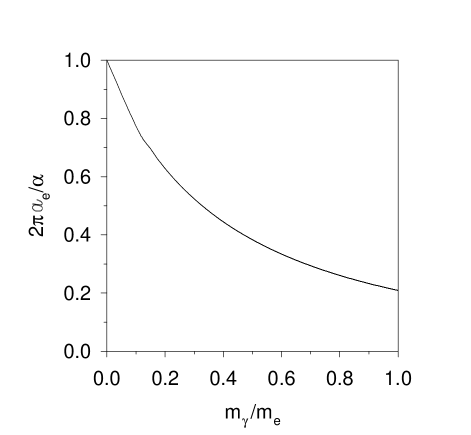
FIG. 2.: The one-photon perturbative contribution to the anomalous moment $a_{e}$ as a function of photon mass $m_{\gamma}$. It is the Schwinger term, given by Eq. 13 of the text.

B Discretization

The most systematic approach to discretization of the eigenvalue problem is the method originally suggested by Pauli and Brodsky[6], discretized light-cone quantization (DLCQ). In essence it is the replacement of integrals by trapezoidal approximations, with equally-spaced intervals in the longitudinal and transverse momenta

$$p^{+}\rightarrow\frac{\pi}{L}n\,,\;\;\mathchoice{{\hbox{\boldmath$\displaystyle p$}}}{{\hbox{\boldmath$\textstyle p$}}}{{\hbox{\boldmath$\scriptstyle p$}}}{{\hbox{\boldmath$\scriptscriptstyle p$}}}_{\perp}\rightarrow(\frac{\pi}{L_{\perp}}n_{x},\frac{\pi}{L_{\perp}}n_{y})\,.$$ (14)

The length scales $L$ and $L_{\perp}$ determine the resolution of the calculation. Because the plus component of momentum is always positive, the limit $L\rightarrow\infty$ can be exchanged for a limit in terms of the integer resolution[6]

$$K\equiv\frac{L}{\pi}P^{+}\,.$$ (15)

The combination of momentum components that defines $H_{\rm LC}$ is then independent of $L$. The longitudinal momentum fractions $x_{i}$ become ratios of integers $n_{i}/K$. Because the $n_{i}$ are all positive, DLCQ automatically limits the number of particles to no more than $K$. The integers $n_{x}$ and $n_{y}$ range between limits associated with some maximum integer $N_{\perp}$ fixed by the invariant-mass cutoff. A finite matrix problem is then obtained without an explicit Tamm-Dancoff truncation; however, this number of particles is much too large in practice for numerical treatments of three-dimensional theories.

We use antiperiodic boundary conditions for the fermions and periodic boundary conditions for the photons. These restrict the integers $n$ associated with longitudinal momenta to being odd for fermions and even for photons. The description of the dressed electron state must then use odd values of $K$.

In most applications, DLCQ is introduced at the level of second quantization. This can yield a compact expression of the eigenvalue problem. Recently, a transformation of the DLCQ Hamiltonian to a Gaussian basis has been suggested[65]; however, the steps for renormalization in that basis have not been worked out.

The application of DLCQ to QED is summarized in [21], which we use as a starting point. This includes use of light-cone gauge [66], with $A^{+}=0$. Modifications of this gauge choice due to zero modes[57] are discussed in Sec. IV.

FIG. 3.: Complete set of diagrams for the fundamental interactions of QED in light-cone quantization. Solid lines represent fermions; wavy lines represent photons. A line with a bar through it indicates an instantaneous interaction expressed in the Hamiltonian as a four-body operator. Only the first three diagrams are included in the present calculation, and for the third, the piece kinematically equivalent to a Z graph is neglected.

The fundamental interactions of light-cone QED are illustrated in Fig. 3. For the calculation reported here we do not include any pair production processes. The instantaneous photon interactions are then completely excluded because each Fock state has only one fermion. We also exclude the fourth diagram (and its conjugate) to decouple two-photon states from the bare electron state; this simplifies the calculation and limits the role of two-photon states to that of providing the basis for inclusion of crossed-photon graphs. There is also a technical modification of the interaction associated with the third diagram of Fig. 3 which is discussed in Sec. III C. After the exclusions have been made, the light-cone Hamiltonian becomes

$$H_{\rm LC}=\sum_{\underline{n}}\sum_{s=\pm 1/2}\frac{m_{e}^{2}+(\mathchoice{{\hbox{\boldmath$\displaystyle n$}}}{{\hbox{\boldmath$\textstyle n$}}}{{\hbox{\boldmath$\scriptstyle n$}}}{{\hbox{\boldmath$\scriptscriptstyle n$}}}_{\perp}\pi/L_{\perp})^{2}}{n/K}b_{\underline{n},s}^{\dagger}b_{\underline{n},s}+\sum_{\underline{m}}\sum_{\lambda=\pm 1}\frac{m_{e}^{2}+(\mathchoice{{\hbox{\boldmath$\displaystyle m$}}}{{\hbox{\boldmath$\textstyle m$}}}{{\hbox{\boldmath$\scriptstyle m$}}}{{\hbox{\boldmath$\scriptscriptstyle m$}}}_{\perp}\pi/L_{\perp})^{2}}{m/K}a_{\underline{m},\lambda}^{\dagger}a_{\underline{m},\lambda}$$ (21)

$$+\frac{eKm_{e}}{2\sqrt{\pi}L_{\perp}}\sum_{\underline{n}_{1},\underline{n}_{2},\underline{m}}\sum_{s=\pm 1/2}\frac{1}{\sqrt{m}}\left\{\delta_{\underline{n}_{1}+\underline{m},\underline{n}_{2}}\left(\frac{1}{n_{1}}-\frac{1}{n_{2}}\right)b_{\underline{n}_{2},s}^{\dagger}b_{\underline{n}_{1},-s}a_{\underline{m},2s}+\,\mbox{h.c.}\right\}$$

$$+\frac{e\sqrt{\pi}K}{\sqrt{2}L_{\perp}^{2}}\sum_{\underline{n}_{1},\underline{n}_{2},\underline{m}}\sum_{s=\pm 1/2}\frac{1}{\sqrt{m}}\delta_{\underline{n}_{1}+\underline{m},\underline{n}_{2}}\left\{\mathchoice{{\hbox{\boldmath$\displaystyle\epsilon$}}}{{\hbox{\boldmath$\textstyle\epsilon$}}}{{\hbox{\boldmath$\scriptstyle\epsilon$}}}{{\hbox{\boldmath$\scriptscriptstyle\epsilon$}}}_{\perp\,,2s}\cdot\left(\frac{\mathchoice{{\hbox{\boldmath$\displaystyle m$}}}{{\hbox{\boldmath$\textstyle m$}}}{{\hbox{\boldmath$\scriptstyle m$}}}{{\hbox{\boldmath$\scriptscriptstyle m$}}}_{\perp}}{m}-\frac{\mathchoice{{\hbox{\boldmath$\displaystyle n$}}}{{\hbox{\boldmath$\textstyle n$}}}{{\hbox{\boldmath$\scriptstyle n$}}}{{\hbox{\boldmath$\scriptscriptstyle n$}}}_{\perp 1}}{n_{1}}\right)b_{\underline{n}_{2},s}^{\dagger}b_{\underline{n}_{1},s}a_{\underline{m},2s}+\,\mbox{h.c.}\right.$$

$$\hskip 108.405pt+\left.\mathchoice{{\hbox{\boldmath$\displaystyle\epsilon$}}}{{\hbox{\boldmath$\textstyle\epsilon$}}}{{\hbox{\boldmath$\scriptstyle\epsilon$}}}{{\hbox{\boldmath$\scriptscriptstyle\epsilon$}}}_{\perp\,,-2s}\cdot\left(\frac{\mathchoice{{\hbox{\boldmath$\displaystyle m$}}}{{\hbox{\boldmath$\textstyle m$}}}{{\hbox{\boldmath$\scriptstyle m$}}}{{\hbox{\boldmath$\scriptscriptstyle m$}}}_{\perp}}{m}-\frac{\mathchoice{{\hbox{\boldmath$\displaystyle n$}}}{{\hbox{\boldmath$\textstyle n$}}}{{\hbox{\boldmath$\scriptstyle n$}}}{{\hbox{\boldmath$\scriptscriptstyle n$}}}_{\perp 2}}{n_{2}}\right)b_{\underline{n}_{2},s}^{\dagger}b_{\underline{n}_{1},s}a_{\underline{m},-2s}+\,\mbox{h.c.}\right\}$$

$$+\frac{e^{2}K}{4\pi L_{\perp}^{2}}\sum_{\underline{n}_{1},\underline{n}_{2},\underline{m}_{1},\underline{m}_{2}}\sum_{s=\pm 1/2}\frac{1}{\sqrt{m_{1}m_{2}}}\delta_{\underline{n}_{2}+\underline{m}_{2},\underline{n}_{1}+\underline{m}_{1}}\left\{\frac{1}{n_{1}+m_{1}}b_{\underline{n}_{2},s}^{\dagger}b_{\underline{n}_{1},s}a_{\underline{m}_{2},-2s}^{\dagger}a_{\underline{m}_{1},-2s}\right.$$

$$\hskip 108.405pt+\left.\frac{1}{m_{2}-n_{1}}b_{\underline{n}_{2},s}^{\dagger}b_{\underline{n}_{1},s}a_{\underline{m}_{2},2s}^{\dagger}a_{\underline{m}_{1},2s}\right\}\,.$$

with $\mathchoice{{\hbox{\boldmath$\displaystyle\epsilon$}}}{{\hbox{\boldmath$\textstyle\epsilon$}}}{{\hbox{\boldmath$\scriptstyle\epsilon$}}}{{\hbox{\boldmath$\scriptscriptstyle\epsilon$}}}_{\perp\,,\lambda}=-(\lambda,i)/\sqrt{2}$.

The discrete form of the spin-$s$ eigenstate $\Psi_{s}$ is

$$\Psi_{s} = \psi_{0s}b_{\underline{K},s}^{\dagger}|0\rangle+\sum_{\underline{n},\underline{m}}\delta_{\underline{n}+\underline{m},\underline{K}}\sum_{s_{1},\lambda_{1}}\psi_{1s}(\underline{n},\underline{m};s_{1},\lambda_{1})b_{\underline{n},s_{1}}^{\dagger}a_{\underline{m},\lambda_{1}}^{\dagger}|0\rangle$$ (23)

$$+\sum_{\underline{n},\underline{m}_{1},\underline{m}_{2}}\delta_{\underline{n}+\underline{m}_{1}+\underline{m}_{2},\underline{K}}\sum_{s_{1},\lambda_{1},\lambda_{2}}\psi_{2s}(\underline{n},\underline{m}_{1},\underline{m}_{2};s_{1},\lambda_{1},\lambda_{2})\frac{1}{\sqrt{2}}b_{\underline{n},s_{1}}^{\dagger}a_{\underline{m}_{1},\lambda_{1}}^{\dagger}a_{\underline{m}_{2},\lambda_{2}}^{\dagger}|0\rangle\,,$$

where $\underline{K}=(K,\mathchoice{{\hbox{\boldmath$\displaystyle K$}}}{{\hbox{\boldmath$\textstyle K$}}}{{\hbox{\boldmath$\scriptstyle K$}}}{{\hbox{\boldmath$\scriptscriptstyle K$}}}_{\perp}=0)$. According to the eigenvalue equation $H_{\rm LC}\Psi=M^{2}\Psi$ the amplitudes $\psi_{is}$ must satisfy the following (discretized) integral equations:

$$(M^{2}-m_{0}^{2})\psi_{0s}=e_{0}\frac{Km_{e}}{2\sqrt{\pi}L_{\perp}}\sum_{\underline{n},\underline{m}}\delta_{\underline{n}+\underline{m},\underline{K}}\frac{1}{\sqrt{m}}\left(\frac{1}{n}-\frac{1}{K}\right)\psi_{1s}(\underline{n},\underline{m};-s,2s)$$ (26)

$$+e_{0}\frac{K\sqrt{\pi}}{\sqrt{2}L_{\perp}^{2}}\sum_{\underline{n},\underline{m}}\delta_{\underline{n}+\underline{m},\underline{K}}\frac{1}{\sqrt{m}}\left\{\mathchoice{{\hbox{\boldmath$\displaystyle\epsilon$}}}{{\hbox{\boldmath$\textstyle\epsilon$}}}{{\hbox{\boldmath$\scriptstyle\epsilon$}}}{{\hbox{\boldmath$\scriptscriptstyle\epsilon$}}}_{\perp\,,2s}\cdot\left(\frac{\mathchoice{{\hbox{\boldmath$\displaystyle m$}}}{{\hbox{\boldmath$\textstyle m$}}}{{\hbox{\boldmath$\scriptstyle m$}}}{{\hbox{\boldmath$\scriptscriptstyle m$}}}_{\perp}}{m}-\frac{\mathchoice{{\hbox{\boldmath$\displaystyle n$}}}{{\hbox{\boldmath$\textstyle n$}}}{{\hbox{\boldmath$\scriptstyle n$}}}{{\hbox{\boldmath$\scriptscriptstyle n$}}}_{\perp}}{n}\right)\psi_{1s}(\underline{n},\underline{m};s,2s)\right.$$

$$\hskip 108.405pt+\left.\mathchoice{{\hbox{\boldmath$\displaystyle\epsilon$}}}{{\hbox{\boldmath$\textstyle\epsilon$}}}{{\hbox{\boldmath$\scriptstyle\epsilon$}}}{{\hbox{\boldmath$\scriptscriptstyle\epsilon$}}}_{\perp\,,-2s}\cdot\frac{\mathchoice{{\hbox{\boldmath$\displaystyle m$}}}{{\hbox{\boldmath$\textstyle m$}}}{{\hbox{\boldmath$\scriptstyle m$}}}{{\hbox{\boldmath$\scriptscriptstyle m$}}}_{\perp}}{m}\psi_{1s}(\underline{n},\underline{m};s,-2s)\right\}\,,$$

$$\left(M^{2}-\left[\frac{m_{1}^{2}(\underline{n}^{\prime})+(\mathchoice{{\hbox{\boldmath$\displaystyle n$}}}{{\hbox{\boldmath$\textstyle n$}}}{{\hbox{\boldmath$\scriptstyle n$}}}{{\hbox{\boldmath$\scriptscriptstyle n$}}}^{\prime}_{\perp}\pi/L_{\perp})^{2}}{n^{\prime}/K}+\frac{m_{\gamma}^{2}+(\mathchoice{{\hbox{\boldmath$\displaystyle m$}}}{{\hbox{\boldmath$\textstyle m$}}}{{\hbox{\boldmath$\scriptstyle m$}}}{{\hbox{\boldmath$\scriptscriptstyle m$}}}^{\prime}_{\perp}\pi/L_{\perp})^{2}}{m^{\prime}/K}\right]\right)\psi_{1s}(\underline{n}^{\prime},\underline{m}^{\prime};s_{1},\lambda_{1})$$ (37)

$$=\frac{K}{4\pi L_{\perp}^{2}}\sum_{\underline{n},\underline{m}}\delta_{\underline{n}+\underline{m},\underline{K}}\frac{1}{\sqrt{m^{\prime}m}}\left\{e_{0}^{2}\delta_{\lambda_{1},-2s_{1}}\frac{1}{K}\psi_{1s}(\underline{n},\underline{m};s_{1},-2s_{1})\right.$$

$$\hskip 72.26999pt\left.-e_{1}(\underline{n}^{\prime})e_{1}(\underline{n})\delta_{\lambda_{1},2s_{1}}\frac{\theta(n-m^{\prime})}{n-m^{\prime}}\psi_{1s}(\underline{n},\underline{m};s_{1},2s_{1})\right\}$$

$$+e_{0}\frac{Km_{e}}{2\sqrt{\pi}L_{\perp}}\frac{1}{\sqrt{m^{\prime}}}\left(\frac{1}{n^{\prime}}-\frac{1}{K}\right)\delta_{\lambda_{1},2s}\delta_{s_{1},-s}\psi_{0s}$$

$$+e_{0}\frac{K\sqrt{\pi}}{\sqrt{2}L_{\perp}^{2}}\frac{1}{\sqrt{m^{\prime}}}\left\{\mathchoice{{\hbox{\boldmath$\displaystyle\epsilon$}}}{{\hbox{\boldmath$\textstyle\epsilon$}}}{{\hbox{\boldmath$\scriptstyle\epsilon$}}}{{\hbox{\boldmath$\scriptscriptstyle\epsilon$}}}_{\perp\,,\lambda_{1}}^{*}\cdot\left(\frac{\mathchoice{{\hbox{\boldmath$\displaystyle m$}}}{{\hbox{\boldmath$\textstyle m$}}}{{\hbox{\boldmath$\scriptstyle m$}}}{{\hbox{\boldmath$\scriptscriptstyle m$}}}^{\prime}_{\perp}}{m^{\prime}}-\frac{\mathchoice{{\hbox{\boldmath$\displaystyle n$}}}{{\hbox{\boldmath$\textstyle n$}}}{{\hbox{\boldmath$\scriptstyle n$}}}{{\hbox{\boldmath$\scriptscriptstyle n$}}}^{\prime}_{\perp}}{n^{\prime}}\right)\delta_{\lambda_{1},2s}\delta_{s_{1},s}+\mathchoice{{\hbox{\boldmath$\displaystyle\epsilon$}}}{{\hbox{\boldmath$\textstyle\epsilon$}}}{{\hbox{\boldmath$\scriptstyle\epsilon$}}}{{\hbox{\boldmath$\scriptscriptstyle\epsilon$}}}_{\perp\,,\lambda_{1}}^{*}\cdot\frac{\mathchoice{{\hbox{\boldmath$\displaystyle m$}}}{{\hbox{\boldmath$\textstyle m$}}}{{\hbox{\boldmath$\scriptstyle m$}}}{{\hbox{\boldmath$\scriptscriptstyle m$}}}^{\prime}_{\perp}}{m^{\prime}}\delta_{\lambda_{1},-2s}\delta_{s_{1},s}\right\}\psi_{0s}$$

$$+e_{1}(\underline{n}^{\prime})\frac{Km_{e}}{2\sqrt{\pi}L_{\perp}}\sum_{\underline{n},\underline{m}}\delta_{\underline{n}+\underline{m}+\underline{m^{\prime}},\underline{K}}\frac{1}{\sqrt{2m}}\left(\frac{1}{n}-\frac{1}{n+m}\right)$$

$$\hskip 72.26999pt\times\left\{\psi_{2s}(\underline{n},\underline{m},\underline{m}^{\prime};-s_{1},2s_{1},\lambda_{1})+\psi_{2s}(\underline{n},\underline{m}^{\prime},\underline{m};-s_{1},\lambda_{1},2s_{1})\right\}$$

$$+e_{1}(\underline{n}^{\prime})\frac{K\sqrt{\pi}}{\sqrt{2}L_{\perp}^{2}}\sum_{\underline{n},\underline{m}}\delta_{\underline{n}+\underline{m}+\underline{m^{\prime}},\underline{K}}\frac{1}{\sqrt{2m}}\left\{\mathchoice{{\hbox{\boldmath$\displaystyle\epsilon$}}}{{\hbox{\boldmath$\textstyle\epsilon$}}}{{\hbox{\boldmath$\scriptstyle\epsilon$}}}{{\hbox{\boldmath$\scriptscriptstyle\epsilon$}}}_{\perp\,,2s_{1}}\cdot\left(\frac{\mathchoice{{\hbox{\boldmath$\displaystyle m$}}}{{\hbox{\boldmath$\textstyle m$}}}{{\hbox{\boldmath$\scriptstyle m$}}}{{\hbox{\boldmath$\scriptscriptstyle m$}}}_{\perp}}{m}-\frac{\mathchoice{{\hbox{\boldmath$\displaystyle n$}}}{{\hbox{\boldmath$\textstyle n$}}}{{\hbox{\boldmath$\scriptstyle n$}}}{{\hbox{\boldmath$\scriptscriptstyle n$}}}_{\perp}}{n}\right)\psi_{2s}(\underline{n},\underline{m},\underline{m}^{\prime};s_{1},2s_{1},\lambda_{1})\right.$$

$$\hskip 72.26999pt+\mathchoice{{\hbox{\boldmath$\displaystyle\epsilon$}}}{{\hbox{\boldmath$\textstyle\epsilon$}}}{{\hbox{\boldmath$\scriptstyle\epsilon$}}}{{\hbox{\boldmath$\scriptscriptstyle\epsilon$}}}_{\perp\,,2s_{1}}\cdot\left(\frac{\mathchoice{{\hbox{\boldmath$\displaystyle m$}}}{{\hbox{\boldmath$\textstyle m$}}}{{\hbox{\boldmath$\scriptstyle m$}}}{{\hbox{\boldmath$\scriptscriptstyle m$}}}_{\perp}}{m}-\frac{\mathchoice{{\hbox{\boldmath$\displaystyle n$}}}{{\hbox{\boldmath$\textstyle n$}}}{{\hbox{\boldmath$\scriptstyle n$}}}{{\hbox{\boldmath$\scriptscriptstyle n$}}}_{\perp}}{n}\right)\psi_{2s}(\underline{n},\underline{m}^{\prime},\underline{m};s_{1},\lambda_{1},2s_{1})$$

$$\hskip 72.26999pt+\mathchoice{{\hbox{\boldmath$\displaystyle\epsilon$}}}{{\hbox{\boldmath$\textstyle\epsilon$}}}{{\hbox{\boldmath$\scriptstyle\epsilon$}}}{{\hbox{\boldmath$\scriptscriptstyle\epsilon$}}}_{\perp\,,-2s_{1}}\cdot\left(\frac{\mathchoice{{\hbox{\boldmath$\displaystyle m$}}}{{\hbox{\boldmath$\textstyle m$}}}{{\hbox{\boldmath$\scriptstyle m$}}}{{\hbox{\boldmath$\scriptscriptstyle m$}}}_{\perp}}{m}-\frac{\mathchoice{{\hbox{\boldmath$\displaystyle n$}}}{{\hbox{\boldmath$\textstyle n$}}}{{\hbox{\boldmath$\scriptstyle n$}}}{{\hbox{\boldmath$\scriptscriptstyle n$}}}^{\prime}_{\perp}}{n^{\prime}}\right)\psi_{2s}(\underline{n},\underline{m},\underline{m}^{\prime};s_{1},-2s_{1},\lambda_{1})$$

$$\hskip 72.26999pt\left.+\mathchoice{{\hbox{\boldmath$\displaystyle\epsilon$}}}{{\hbox{\boldmath$\textstyle\epsilon$}}}{{\hbox{\boldmath$\scriptstyle\epsilon$}}}{{\hbox{\boldmath$\scriptscriptstyle\epsilon$}}}_{\perp\,,-2s_{1}}\cdot\left(\frac{\mathchoice{{\hbox{\boldmath$\displaystyle m$}}}{{\hbox{\boldmath$\textstyle m$}}}{{\hbox{\boldmath$\scriptstyle m$}}}{{\hbox{\boldmath$\scriptscriptstyle m$}}}_{\perp}}{m}-\frac{\mathchoice{{\hbox{\boldmath$\displaystyle n$}}}{{\hbox{\boldmath$\textstyle n$}}}{{\hbox{\boldmath$\scriptstyle n$}}}{{\hbox{\boldmath$\scriptscriptstyle n$}}}^{\prime}_{\perp}}{n^{\prime}}\right)\psi_{2s}(\underline{n},\underline{m}^{\prime},\underline{m};s_{1},\lambda_{1},-2s_{1})\right\}\,,$$

and

$$\left(M^{2}-\left[\frac{m_{e}^{2}+(\mathchoice{{\hbox{\boldmath$\displaystyle n$}}}{{\hbox{\boldmath$\textstyle n$}}}{{\hbox{\boldmath$\scriptstyle n$}}}{{\hbox{\boldmath$\scriptscriptstyle n$}}}^{\prime}_{\perp}\pi/L_{\perp})^{2}}{n^{\prime}/K}+\frac{m_{\gamma}^{2}+(\mathchoice{{\hbox{\boldmath$\displaystyle m$}}}{{\hbox{\boldmath$\textstyle m$}}}{{\hbox{\boldmath$\scriptstyle m$}}}{{\hbox{\boldmath$\scriptscriptstyle m$}}}^{\prime}_{\perp 1}\pi/L_{\perp})^{2}}{m^{\prime}_{1}/K}\right.\right.$$ (45)

$$\hskip 144.54pt\left.\left.+\frac{m_{\gamma}^{2}+(\mathchoice{{\hbox{\boldmath$\displaystyle m$}}}{{\hbox{\boldmath$\textstyle m$}}}{{\hbox{\boldmath$\scriptstyle m$}}}{{\hbox{\boldmath$\scriptscriptstyle m$}}}^{\prime}_{\perp 2}\pi/L_{\perp})^{2}}{m^{\prime}_{2}/K}\right]\right)\psi_{2s}(\underline{n}^{\prime},\underline{m}^{\prime}_{1},\underline{m}^{\prime}_{2};s_{1},\lambda_{1},\lambda_{2})$$

$$=\frac{Km_{e}}{2\sqrt{2\pi}L_{\perp}}\left\{\delta_{\lambda_{2},-2s_{1}}\frac{e_{1}(\underline{n}^{\prime}+\underline{m}^{\prime}_{2})}{\sqrt{m^{\prime}_{2}}}\left(\frac{1}{n^{\prime}}-\frac{1}{n^{\prime}+m^{\prime}_{2}}\right)\psi_{1s}(\underline{n}^{\prime}+\underline{m}^{\prime}_{2},\underline{m}^{\prime}_{1};-s_{1},\lambda_{1})\right.$$

$$\hskip 36.135pt\left.+\delta_{\lambda_{1},-2s_{1}}\frac{e_{1}(\underline{n}^{\prime}+\underline{m}^{\prime}_{1})}{\sqrt{m^{\prime}_{1}}}\left(\frac{1}{n^{\prime}}-\frac{1}{n^{\prime}+m^{\prime}_{1}}\right)\psi_{1s}(\underline{n}^{\prime}+\underline{m}^{\prime}_{1},\underline{m}^{\prime}_{2};-s_{1},\lambda_{2})\right\}$$

$$\frac{K\sqrt{\pi}}{2L_{\perp}^{2}}\left\{\delta_{\lambda_{2},2s_{1}}\frac{e_{1}(\underline{n}^{\prime}+\underline{m}^{\prime}_{2})}{\sqrt{m_{2}}}\mathchoice{{\hbox{\boldmath$\displaystyle\epsilon$}}}{{\hbox{\boldmath$\textstyle\epsilon$}}}{{\hbox{\boldmath$\scriptstyle\epsilon$}}}{{\hbox{\boldmath$\scriptscriptstyle\epsilon$}}}_{\perp\,,\lambda_{2}}^{*}\cdot\left(\frac{\mathchoice{{\hbox{\boldmath$\displaystyle m$}}}{{\hbox{\boldmath$\textstyle m$}}}{{\hbox{\boldmath$\scriptstyle m$}}}{{\hbox{\boldmath$\scriptscriptstyle m$}}}^{\prime}_{\perp 2}}{m^{\prime}_{2}}-\frac{\mathchoice{{\hbox{\boldmath$\displaystyle n$}}}{{\hbox{\boldmath$\textstyle n$}}}{{\hbox{\boldmath$\scriptstyle n$}}}{{\hbox{\boldmath$\scriptscriptstyle n$}}}^{\prime}_{\perp}}{n^{\prime}}\right)\psi_{1s}(\underline{n}^{\prime}+\underline{m}^{\prime}_{2},\underline{m}^{\prime}_{1};s_{1},\lambda_{1})\right.$$

$$\hskip 36.135pt+\delta_{\lambda_{1},2s_{1}}\frac{e_{1}(\underline{n}^{\prime}+\underline{m}^{\prime}_{1})}{\sqrt{m_{1}}}\mathchoice{{\hbox{\boldmath$\displaystyle\epsilon$}}}{{\hbox{\boldmath$\textstyle\epsilon$}}}{{\hbox{\boldmath$\scriptstyle\epsilon$}}}{{\hbox{\boldmath$\scriptscriptstyle\epsilon$}}}_{\perp\,,\lambda_{1}}^{*}\cdot\left(\frac{\mathchoice{{\hbox{\boldmath$\displaystyle m$}}}{{\hbox{\boldmath$\textstyle m$}}}{{\hbox{\boldmath$\scriptstyle m$}}}{{\hbox{\boldmath$\scriptscriptstyle m$}}}^{\prime}_{\perp 1}}{m^{\prime}_{1}}-\frac{\mathchoice{{\hbox{\boldmath$\displaystyle n$}}}{{\hbox{\boldmath$\textstyle n$}}}{{\hbox{\boldmath$\scriptstyle n$}}}{{\hbox{\boldmath$\scriptscriptstyle n$}}}^{\prime}_{\perp}}{n^{\prime}}\right)\psi_{1s}(\underline{n}^{\prime}+\underline{m}^{\prime}_{1},\underline{m}^{\prime}_{2};s_{1},\lambda_{2})$$

$$\hskip 36.135pt+\delta_{\lambda_{2},-2s_{1}}\frac{e_{1}(\underline{n}^{\prime}+\underline{m}^{\prime}_{2})}{\sqrt{m_{2}}}\mathchoice{{\hbox{\boldmath$\displaystyle\epsilon$}}}{{\hbox{\boldmath$\textstyle\epsilon$}}}{{\hbox{\boldmath$\scriptstyle\epsilon$}}}{{\hbox{\boldmath$\scriptscriptstyle\epsilon$}}}_{\perp\,,\lambda_{2}}^{*}\cdot\left(\frac{\mathchoice{{\hbox{\boldmath$\displaystyle m$}}}{{\hbox{\boldmath$\textstyle m$}}}{{\hbox{\boldmath$\scriptstyle m$}}}{{\hbox{\boldmath$\scriptscriptstyle m$}}}^{\prime}_{\perp 2}}{m^{\prime}_{2}}-\frac{\mathchoice{{\hbox{\boldmath$\displaystyle n$}}}{{\hbox{\boldmath$\textstyle n$}}}{{\hbox{\boldmath$\scriptstyle n$}}}{{\hbox{\boldmath$\scriptscriptstyle n$}}}^{\prime}_{\perp}+\mathchoice{{\hbox{\boldmath$\displaystyle m$}}}{{\hbox{\boldmath$\textstyle m$}}}{{\hbox{\boldmath$\scriptstyle m$}}}{{\hbox{\boldmath$\scriptscriptstyle m$}}}^{\prime}_{\perp 2}}{n^{\prime}+m^{\prime}_{2}}\right)\psi_{1s}(\underline{n}^{\prime}+\underline{m}^{\prime}_{2},\underline{m}^{\prime}_{1};s_{1},\lambda_{1})$$

$$\hskip 36.135pt\left.+\delta_{\lambda_{1},-2s_{1}}\frac{e_{1}(\underline{n}^{\prime}+\underline{m}^{\prime}_{1})}{\sqrt{m_{1}}}\mathchoice{{\hbox{\boldmath$\displaystyle\epsilon$}}}{{\hbox{\boldmath$\textstyle\epsilon$}}}{{\hbox{\boldmath$\scriptstyle\epsilon$}}}{{\hbox{\boldmath$\scriptscriptstyle\epsilon$}}}_{\perp\,,\lambda_{1}}^{*}\cdot\left(\frac{\mathchoice{{\hbox{\boldmath$\displaystyle m$}}}{{\hbox{\boldmath$\textstyle m$}}}{{\hbox{\boldmath$\scriptstyle m$}}}{{\hbox{\boldmath$\scriptscriptstyle m$}}}^{\prime}_{\perp 1}}{m^{\prime}_{1}}-\frac{\mathchoice{{\hbox{\boldmath$\displaystyle n$}}}{{\hbox{\boldmath$\textstyle n$}}}{{\hbox{\boldmath$\scriptstyle n$}}}{{\hbox{\boldmath$\scriptscriptstyle n$}}}^{\prime}_{\perp}+\mathchoice{{\hbox{\boldmath$\displaystyle m$}}}{{\hbox{\boldmath$\textstyle m$}}}{{\hbox{\boldmath$\scriptstyle m$}}}{{\hbox{\boldmath$\scriptscriptstyle m$}}}^{\prime}_{\perp 1}}{n^{\prime}+m^{\prime}_{1}}\right)\psi_{1s}(\underline{n}^{\prime}+\underline{m}^{\prime}_{1},\underline{m}^{\prime}_{2};s_{1},\lambda_{2})\right\}\,.$$

In anticipation of the discussion of renormalization in Sec. III, bare masses $m_{0}$ and $m_{1}$ and bare couplings $e_{0}$ and $e_{1}$ have been introduced. These equations are solved numerically, with the first step being the use of (45) to eliminate $\psi_{2}$ from (37). Once a solution is obtained for one value of total spin $s$, the solution for the opposite spin can be computed directly from

$$\psi_{1\downarrow}(s_{1}=-1/2,\lambda_{1}=\mp 1)=-\psi_{1\uparrow}^{*}(+1/2,\pm 1)$$ (46)

and

$$\psi_{1\downarrow}(s_{1}=+1/2,\lambda_{1}=\mp 1)=+\psi_{1\uparrow}^{*}(-1/2,\pm 1)\,.$$ (47)

These follow from the symmetries of the integral equations.

Other symmetries lead to relationships between amplitude components, which can be summarized as follows:

$$\psi_{1\uparrow}(x,\mathchoice{{\hbox{\boldmath$\displaystyle k$}}}{{\hbox{\boldmath$\textstyle k$}}}{{\hbox{\boldmath$\scriptstyle k$}}}{{\hbox{\boldmath$\scriptscriptstyle k$}}}_{\perp};s_{1}=1/2,\lambda_{1}=\pm 1)=k_{x}f_{r\lambda_{1}}(|k_{x}|,|k_{y}|)+ik_{y}f_{i\lambda_{1}}(|k_{x}|,|k_{y}|)$$ (48)

and

$$\psi_{1\uparrow}(x,\mathchoice{{\hbox{\boldmath$\displaystyle k$}}}{{\hbox{\boldmath$\textstyle k$}}}{{\hbox{\boldmath$\scriptstyle k$}}}{{\hbox{\boldmath$\scriptscriptstyle k$}}}_{\perp};s_{1}=-1/2,\lambda_{1}=\pm 1)=g_{r\lambda_{1}}(|k_{x}|,|k_{y}|)+ik_{x}k_{y}g_{i\lambda_{1}}(|k_{x}|,|k_{y}|)\,,$$ (49)

where the functions $f_{r\lambda}$, $f_{i\lambda}$, $g_{r\lambda}$, and $g_{i\lambda}$ are real. The problem can then be reduced to a smaller matrix problem for these real functions. For $s_{1}=1/2$ we store $k_{x}f_{r\pm}(k_{x}>0,0)$, $k_{y}f_{i\pm}(0,k_{y}>0)$, $k_{x}f_{r\pm}(k_{x}>0,k_{y}>0)$, and $k_{y}f_{i\pm}(k_{x}>0,k_{y}>0)$. For $s_{1}=-1/2$ we store $g_{r\pm}(0,0)$, $g_{r\pm}(k_{x}>0,0)$, $g_{r\pm}(0,k_{x}>0)$, $g_{r\pm}(k_{x}>0,k_{y}>0)$, and $k_{x}k_{y}g_{i\pm}(k_{x}>0,k_{y}>0)$. The use of symmetry reduces the matrix storage requirement by a factor of 8. The Hermitian matrix of the original eigenvalue equation (37) can be expressed as a real symmetric matrix in the reduced equation by using a two-component representation of complex arithmetic:

$$(c+id)(\alpha+i\beta)\longrightarrow\left(\begin{array}[]{rr}c&-d\\ d&c\end{array}\right)\left(\begin{array}[]{c}\alpha\\ \beta\end{array}\right)$$ (50)

and

$$(\alpha+i\beta)^{*}\longrightarrow\left(\begin{array}[]{rr}1&0\\ 0&-1\end{array}\right)\left(\begin{array}[]{c}\alpha\\ \beta\end{array}\right)\,.$$ (51)

The leading perturbative result[20] is recovered by keeping only $\psi_{0s}$ terms on the right-hand side of (37). This equation can then be immediately solved for $\psi_{1s}$, which can be used to form a discrete approximation to (12). The approximation includes a finite difference approximation to the derivatives that appear in (10) and therefore is not simply a trapezoidal approximation to (12).

C Discretization errors

Results obtained with ordinary DLCQ show an irregular dependence on the numerical parameters $K$ and $N_{\perp}$, which interferes with extrapolation to infinite resolution. The causes of the irregularities have been determined to be the numerical approximation of the derivative in the formula (10) for $a_{e}$ and boundary effects in the numerical integrations. The error in the derivative can be controlled by choosing $N_{\perp}\geq 7$ and $K\geq 21$. The bound on $K$ is consistent with the resolution needed to resolve the one-photon peak in the $a_{e}$ integrand when $m_{\gamma}=m_{e}/10$, which is the photon mass we use. Smaller values of $m_{\gamma}$ shift the peak to smaller photon momenta and would increase the lower bound on $K$. The shape of the integrand for various values of $m_{\gamma}$ is illustrated in Fig. 4. The mass sensitivity of the numerical convergence rate is shown in Table I.

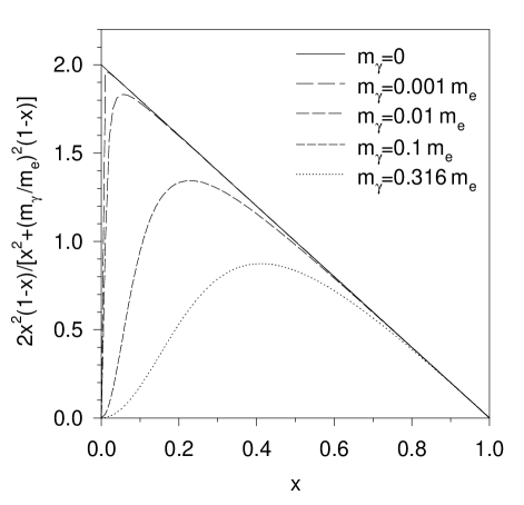
FIG. 4.: The integrand for the one-photon perturbative contribution. The integrals over the transverse momentum have been performed and only the integral over longitudinal momentum $x$ remains, as given in Eq. (13).

TABLE I.: The DLCQ approximation to the perturbative one-photon integral in Eq. (13). The values at different DLCQ resolutions $K$ show that the convergence rate depends on the photon mass $m_{\gamma}$.

	$m_{\gamma}/m_{e}$
$K$	$0$	$0.001$	$0.01$	$0.1$	$0.3162$
11	$0.8182$	$0.8182$	$0.8173$	$0.7455$	$0.5041$
21	$0.9048$	$0.9047$	$0.9025$	$0.7708$	$0.5079$
41	$0.9512$	$0.9512$	$0.9461$	$0.7728$	$0.5090$
81	$0.9753$	$0.9752$	$0.9648$	$0.7731$	$0.5093$
161	$0.9876$	$0.9873$	$0.9699$	$0.7732$	$0.5094$
321	$0.9938$	$0.9933$	$0.9703$	$0.7732$	$0.5094$
641	$0.9969$	$0.9959$	$0.9703$	$0.7732$	$0.5094$
1281	$0.9984$	$0.9968$	$0.9703$	$0.7732$	$0.5094$
2561	$0.9992$	$0.9969$	$0.9703$	$0.7732$	$0.5094$
$\infty$	$1.0000$	$0.9969$	$0.9703$	$0.7732$	$0.5094$

The integration boundary effects are more difficult to control. These effects arise from use of the DLCQ grid which is incommensurate with the integration domain. At the boundaries, the trapezoidal rule misses contributions beyond the last grid point; this error is not a smooth function of the grid spacing. To overcome this error, one can replace the trapezoidal rule by open-closed Newton–Cotes formulas tailored specifically to the boundary [17]. Grid points near the boundary are then associated with unequal integration weights. The unequal weights must be taken into account in normalization sums and symmetrization of the Hamiltonian matrix, but this is easily done. One can even consider use of Simpson’s rule, although this does not appear useful in the anomalous moment calculation. The improvement brought by these weighting methods can be dramatic, as shown in Ref. [17].

III Renormalization

A Mass renormalization

Here we are interested in ultraviolet divergences associated with large $k_{\perp}$. Electron self-energy contributions, which are divergent, shift the mass and, through wave function renormalization, change the coupling. These induce $\Lambda^{2}$ and $\log\Lambda$ dependencies in the eigenvalues. In the discrete truncated problem these effects depend on the Fock sector considered[10]. For example, an electron in a Fock state for which a transition to a state with more photons is not allowed, perhaps due to truncation in photon number, will not experience any self-energy corrections. If one additional photon is allowed, but not instantaneous interactions, only single loops can occur. If two or more additional photons can appear, then an infinite number of overlapping loops can contribute to self-energy corrections, a truly nonperturbative situation. In each case, the leading divergence is removed by introduction of counterterms associated with bare masses that are sector dependent and momentum dependent[67].

To be specific, consider the case where there are at most two photons and only one electron. The Fock-state expansion can be written schematically as

$$\Psi=\psi_{0}|e\rangle+\mathchoice{{\hbox{\boldmath$\displaystyle\psi$}}}{{\hbox{\boldmath$\textstyle\psi$}}}{{\hbox{\boldmath$\scriptstyle\psi$}}}{{\hbox{\boldmath$\scriptscriptstyle\psi$}}}_{1}|e\gamma\rangle+\mathchoice{{\hbox{\boldmath$\displaystyle\psi$}}}{{\hbox{\boldmath$\textstyle\psi$}}}{{\hbox{\boldmath$\scriptstyle\psi$}}}{{\hbox{\boldmath$\scriptscriptstyle\psi$}}}_{2}|e\gamma\gamma\rangle\,.$$ (52)

Here $\mathchoice{{\hbox{\boldmath$\displaystyle\psi$}}}{{\hbox{\boldmath$\textstyle\psi$}}}{{\hbox{\boldmath$\scriptstyle\psi$}}}{{\hbox{\boldmath$\scriptscriptstyle\psi$}}}_{1}$ and $\mathchoice{{\hbox{\boldmath$\displaystyle\psi$}}}{{\hbox{\boldmath$\textstyle\psi$}}}{{\hbox{\boldmath$\scriptstyle\psi$}}}{{\hbox{\boldmath$\scriptscriptstyle\psi$}}}_{2}$ are column vectors that contain the amplitudes for individual Fock states with one and two photons, respectively. The eigenvalue problem (4) becomes a coupled set of three integral equations (26), (37), and (45), which we write more compactly as

$$m_{0}^{2}\psi_{0}+\mathchoice{{\hbox{\boldmath$\displaystyle b$}}}{{\hbox{\boldmath$\textstyle b$}}}{{\hbox{\boldmath$\scriptstyle b$}}}{{\hbox{\boldmath$\scriptscriptstyle b$}}}_{1}^{\dagger}\cdot\mathchoice{{\hbox{\boldmath$\displaystyle\psi$}}}{{\hbox{\boldmath$\textstyle\psi$}}}{{\hbox{\boldmath$\scriptstyle\psi$}}}{{\hbox{\boldmath$\scriptscriptstyle\psi$}}}_{1}+\mathchoice{{\hbox{\boldmath$\displaystyle b$}}}{{\hbox{\boldmath$\textstyle b$}}}{{\hbox{\boldmath$\scriptstyle b$}}}{{\hbox{\boldmath$\scriptscriptstyle b$}}}_{2}^{\dagger}\cdot\mathchoice{{\hbox{\boldmath$\displaystyle\psi$}}}{{\hbox{\boldmath$\textstyle\psi$}}}{{\hbox{\boldmath$\scriptstyle\psi$}}}{{\hbox{\boldmath$\scriptscriptstyle\psi$}}}_{2} = M^{2}\psi_{0}\,,$$ (53)

$$\mathchoice{{\hbox{\boldmath$\displaystyle b$}}}{{\hbox{\boldmath$\textstyle b$}}}{{\hbox{\boldmath$\scriptstyle b$}}}{{\hbox{\boldmath$\scriptscriptstyle b$}}}_{1}\psi_{0}+\mathchoice{{\hbox{\boldmath$\displaystyle A$}}}{{\hbox{\boldmath$\textstyle A$}}}{{\hbox{\boldmath$\scriptstyle A$}}}{{\hbox{\boldmath$\scriptscriptstyle A$}}}_{11}\mathchoice{{\hbox{\boldmath$\displaystyle\psi$}}}{{\hbox{\boldmath$\textstyle\psi$}}}{{\hbox{\boldmath$\scriptstyle\psi$}}}{{\hbox{\boldmath$\scriptscriptstyle\psi$}}}_{1}+\mathchoice{{\hbox{\boldmath$\displaystyle A$}}}{{\hbox{\boldmath$\textstyle A$}}}{{\hbox{\boldmath$\scriptstyle A$}}}{{\hbox{\boldmath$\scriptscriptstyle A$}}}_{12}\mathchoice{{\hbox{\boldmath$\displaystyle\psi$}}}{{\hbox{\boldmath$\textstyle\psi$}}}{{\hbox{\boldmath$\scriptstyle\psi$}}}{{\hbox{\boldmath$\scriptscriptstyle\psi$}}}_{2} = M^{2}\mathchoice{{\hbox{\boldmath$\displaystyle\psi$}}}{{\hbox{\boldmath$\textstyle\psi$}}}{{\hbox{\boldmath$\scriptstyle\psi$}}}{{\hbox{\boldmath$\scriptscriptstyle\psi$}}}_{1}\,,$$ (54)

$$\mathchoice{{\hbox{\boldmath$\displaystyle b$}}}{{\hbox{\boldmath$\textstyle b$}}}{{\hbox{\boldmath$\scriptstyle b$}}}{{\hbox{\boldmath$\scriptscriptstyle b$}}}_{2}\psi_{0}+\mathchoice{{\hbox{\boldmath$\displaystyle A$}}}{{\hbox{\boldmath$\textstyle A$}}}{{\hbox{\boldmath$\scriptstyle A$}}}{{\hbox{\boldmath$\scriptscriptstyle A$}}}_{12}^{\dagger}\mathchoice{{\hbox{\boldmath$\displaystyle\psi$}}}{{\hbox{\boldmath$\textstyle\psi$}}}{{\hbox{\boldmath$\scriptstyle\psi$}}}{{\hbox{\boldmath$\scriptscriptstyle\psi$}}}_{1}+\mathchoice{{\hbox{\boldmath$\displaystyle A$}}}{{\hbox{\boldmath$\textstyle A$}}}{{\hbox{\boldmath$\scriptstyle A$}}}{{\hbox{\boldmath$\scriptscriptstyle A$}}}_{22}\mathchoice{{\hbox{\boldmath$\displaystyle\psi$}}}{{\hbox{\boldmath$\textstyle\psi$}}}{{\hbox{\boldmath$\scriptstyle\psi$}}}{{\hbox{\boldmath$\scriptscriptstyle\psi$}}}_{2} = M^{2}\mathchoice{{\hbox{\boldmath$\displaystyle\psi$}}}{{\hbox{\boldmath$\textstyle\psi$}}}{{\hbox{\boldmath$\scriptstyle\psi$}}}{{\hbox{\boldmath$\scriptscriptstyle\psi$}}}_{2}\,,$$ (55)

where $m_{0}$ is the bare electron mass and the vectors $\mathchoice{{\hbox{\boldmath$\displaystyle b$}}}{{\hbox{\boldmath$\textstyle b$}}}{{\hbox{\boldmath$\scriptstyle b$}}}{{\hbox{\boldmath$\scriptscriptstyle b$}}}_{i}^{\dagger}$ and the tensors $\mathchoice{{\hbox{\boldmath$\displaystyle A$}}}{{\hbox{\boldmath$\textstyle A$}}}{{\hbox{\boldmath$\scriptstyle A$}}}{{\hbox{\boldmath$\scriptscriptstyle A$}}}_{ij}$ are integral operators obtained from $H_{\rm LC}$. We now require that $m_{0}$ be such that $M^{2}=m_{e}^{2}$ is an eigenvalue. The second and third equations can be solved for $\mathchoice{{\hbox{\boldmath$\displaystyle\psi$}}}{{\hbox{\boldmath$\textstyle\psi$}}}{{\hbox{\boldmath$\scriptstyle\psi$}}}{{\hbox{\boldmath$\scriptscriptstyle\psi$}}}_{1}/\psi_{0}$ and $\mathchoice{{\hbox{\boldmath$\displaystyle\psi$}}}{{\hbox{\boldmath$\textstyle\psi$}}}{{\hbox{\boldmath$\scriptstyle\psi$}}}{{\hbox{\boldmath$\scriptscriptstyle\psi$}}}_{2}/\psi_{0}$. Then the first equation yields $m_{0}$. Normalization of $\Psi$ fixes the value of $\psi_{0}$.

Suppose now that this two-photon problem is embedded in some larger problem where one needs to know the bare mass of an electron in a Fock state that can couple to Fock states obtained by adding at most two photons. The same set of equations can be applied, with all constituents in the lowest Fock state, other than the electron, acting as spectators. One need only replace $m_{0}^{2}$ in (53) by $(m_{0}^{2}+k_{\perp}^{2})/x$ and $M^{2}=m_{e}^{2}$ by $M^{2}=(m_{e}^{2}+k_{\perp}^{2})/x$, with $x$ and $\mathchoice{{\hbox{\boldmath$\displaystyle k$}}}{{\hbox{\boldmath$\textstyle k$}}}{{\hbox{\boldmath$\scriptstyle k$}}}{{\hbox{\boldmath$\scriptscriptstyle k$}}}_{\perp}$ the longitudinal momentum fraction and transverse momentum of the initial electron. Notice that $m_{0}$ is now a function of $x$ and $\mathchoice{{\hbox{\boldmath$\displaystyle k$}}}{{\hbox{\boldmath$\textstyle k$}}}{{\hbox{\boldmath$\scriptstyle k$}}}{{\hbox{\boldmath$\scriptscriptstyle k$}}}_{\perp}$.

This can be generalized to cases with more photons, and reduced to the case of only one contributing photon. Thus one obtains a mechanism for a sector-dependent, momentum-dependent mass renormalization that is used from the top $n$-photon sector down to the bare electron state $|e\rangle$. The last step automatically includes the solution of the full eigenvalue problem for the dressed electron state.

For the one-photon case embedded in the two-photon problem we have

$$\frac{m_{1}^{2}+k_{\perp}^{2}}{x}\psi_{1s}(x,\mathchoice{{\hbox{\boldmath$\displaystyle k$}}}{{\hbox{\boldmath$\textstyle k$}}}{{\hbox{\boldmath$\scriptstyle k$}}}{{\hbox{\boldmath$\scriptscriptstyle k$}}}_{\perp})+\mathchoice{{\hbox{\boldmath$\displaystyle b$}}}{{\hbox{\boldmath$\textstyle b$}}}{{\hbox{\boldmath$\scriptstyle b$}}}{{\hbox{\boldmath$\scriptscriptstyle b$}}}^{\dagger}(x,\mathchoice{{\hbox{\boldmath$\displaystyle k$}}}{{\hbox{\boldmath$\textstyle k$}}}{{\hbox{\boldmath$\scriptstyle k$}}}{{\hbox{\boldmath$\scriptscriptstyle k$}}}_{\perp})\cdot\mathchoice{{\hbox{\boldmath$\displaystyle\psi$}}}{{\hbox{\boldmath$\textstyle\psi$}}}{{\hbox{\boldmath$\scriptstyle\psi$}}}{{\hbox{\boldmath$\scriptscriptstyle\psi$}}}_{2} = \frac{m_{e}^{2}+k_{\perp}^{2}}{x}\psi_{1s}(x,\mathchoice{{\hbox{\boldmath$\displaystyle k$}}}{{\hbox{\boldmath$\textstyle k$}}}{{\hbox{\boldmath$\scriptstyle k$}}}{{\hbox{\boldmath$\scriptscriptstyle k$}}}_{\perp})\,,$$ (56)

$$\mathchoice{{\hbox{\boldmath$\displaystyle b$}}}{{\hbox{\boldmath$\textstyle b$}}}{{\hbox{\boldmath$\scriptstyle b$}}}{{\hbox{\boldmath$\scriptscriptstyle b$}}}\,\psi_{1s}(x,\mathchoice{{\hbox{\boldmath$\displaystyle k$}}}{{\hbox{\boldmath$\textstyle k$}}}{{\hbox{\boldmath$\scriptstyle k$}}}{{\hbox{\boldmath$\scriptscriptstyle k$}}}_{\perp})+\mathchoice{{\hbox{\boldmath$\displaystyle A$}}}{{\hbox{\boldmath$\textstyle A$}}}{{\hbox{\boldmath$\scriptstyle A$}}}{{\hbox{\boldmath$\scriptscriptstyle A$}}}\mathchoice{{\hbox{\boldmath$\displaystyle\psi$}}}{{\hbox{\boldmath$\textstyle\psi$}}}{{\hbox{\boldmath$\scriptstyle\psi$}}}{{\hbox{\boldmath$\scriptscriptstyle\psi$}}}_{2} = \frac{m_{e}^{2}+k_{\perp}^{2}}{x}\mathchoice{{\hbox{\boldmath$\displaystyle\psi$}}}{{\hbox{\boldmath$\textstyle\psi$}}}{{\hbox{\boldmath$\scriptstyle\psi$}}}{{\hbox{\boldmath$\scriptscriptstyle\psi$}}}_{2s}\,.$$ (57)

The second photon is a spectator. The coupling to $\mathchoice{{\hbox{\boldmath$\displaystyle\psi$}}}{{\hbox{\boldmath$\textstyle\psi$}}}{{\hbox{\boldmath$\scriptstyle\psi$}}}{{\hbox{\boldmath$\scriptscriptstyle\psi$}}}_{2}$ then induces the one-loop self-energy correction with this spectator present. The explicit form is obtained from (37) and (45) with $M^{2}=(m_{e}^{2}+k_{\perp}^{2})/x+(m_{\gamma}^{2}+k_{\perp}^{2})/(1-x)$ and with any interaction involving the spectator dropped. Eq. 45 can then be solved for $\mathchoice{{\hbox{\boldmath$\displaystyle\psi$}}}{{\hbox{\boldmath$\textstyle\psi$}}}{{\hbox{\boldmath$\scriptstyle\psi$}}}{{\hbox{\boldmath$\scriptscriptstyle\psi$}}}_{2}$ and the result substituted into the modified (37) to obtain.

$$\frac{m_{e}^{2}+(\mathchoice{{\hbox{\boldmath$\displaystyle n$}}}{{\hbox{\boldmath$\textstyle n$}}}{{\hbox{\boldmath$\scriptstyle n$}}}{{\hbox{\boldmath$\scriptscriptstyle n$}}}^{\prime}_{\perp}\pi/L_{\perp})^{2}}{n^{\prime}/K}\psi_{1s}(\underline{n}^{\prime},\underline{m}^{\prime};s_{1},\lambda_{1})=\frac{m_{1}^{2}(\underline{n}^{\prime})+(\mathchoice{{\hbox{\boldmath$\displaystyle n$}}}{{\hbox{\boldmath$\textstyle n$}}}{{\hbox{\boldmath$\scriptstyle n$}}}{{\hbox{\boldmath$\scriptscriptstyle n$}}}^{\prime}_{\perp}\pi/L_{\perp})^{2}}{n^{\prime}/K}\psi_{1s}(\underline{n}^{\prime},\underline{m}^{\prime};s_{1},\lambda_{1})\hskip 36.135pt$$ (60)

$$\hskip 18.06749pt+e_{1}^{2}(\underline{n}^{\prime})\frac{K^{2}m_{e}^{2}}{4\pi L_{\perp}^{2}}\sum_{\underline{n},\underline{m}}\frac{\delta_{\underline{n}+\underline{m},\underline{n}^{\prime}}/m\left(1/n^{\prime}-1/n\right)^{2}\psi_{1s}(\underline{n}^{\prime},\underline{m}^{\prime};s_{1},\lambda_{1})}{\frac{K}{n^{\prime}}\left[m_{e}^{2}+(\mathchoice{{\hbox{\boldmath$\displaystyle n$}}}{{\hbox{\boldmath$\textstyle n$}}}{{\hbox{\boldmath$\scriptstyle n$}}}{{\hbox{\boldmath$\scriptscriptstyle n$}}}^{\prime}_{\perp}\pi/L_{\perp})^{2}\right]-\frac{K}{n}\left[m_{e}^{2}+(\mathchoice{{\hbox{\boldmath$\displaystyle n$}}}{{\hbox{\boldmath$\textstyle n$}}}{{\hbox{\boldmath$\scriptstyle n$}}}{{\hbox{\boldmath$\scriptscriptstyle n$}}}_{\perp}\pi/L_{\perp})^{2}\right]-\frac{K}{m}\left[m_{\gamma}^{2}+(\mathchoice{{\hbox{\boldmath$\displaystyle m$}}}{{\hbox{\boldmath$\textstyle m$}}}{{\hbox{\boldmath$\scriptstyle m$}}}{{\hbox{\boldmath$\scriptscriptstyle m$}}}_{\perp}\pi/L_{\perp})^{2}\right]}$$

$$\hskip 18.06749pt+e_{1}^{2}(\underline{n}^{\prime})\frac{K^{2}\pi}{4L_{\perp}^{4}}\sum_{\underline{n},\underline{m}}\frac{\delta_{\underline{n}+\underline{m},\underline{n}^{\prime}}/m\left\{\left(\mathchoice{{\hbox{\boldmath$\displaystyle m$}}}{{\hbox{\boldmath$\textstyle m$}}}{{\hbox{\boldmath$\scriptstyle m$}}}{{\hbox{\boldmath$\scriptscriptstyle m$}}}_{\perp}/m-\mathchoice{{\hbox{\boldmath$\displaystyle n$}}}{{\hbox{\boldmath$\textstyle n$}}}{{\hbox{\boldmath$\scriptstyle n$}}}{{\hbox{\boldmath$\scriptscriptstyle n$}}}_{\perp}/n\right)^{2}+\left(\mathchoice{{\hbox{\boldmath$\displaystyle m$}}}{{\hbox{\boldmath$\textstyle m$}}}{{\hbox{\boldmath$\scriptstyle m$}}}{{\hbox{\boldmath$\scriptscriptstyle m$}}}_{\perp}/m-\mathchoice{{\hbox{\boldmath$\displaystyle n$}}}{{\hbox{\boldmath$\textstyle n$}}}{{\hbox{\boldmath$\scriptstyle n$}}}{{\hbox{\boldmath$\scriptscriptstyle n$}}}^{\prime}_{\perp}/n^{\prime}\right)^{2}\right\}\psi_{1s}(\underline{n}^{\prime},\underline{m}^{\prime};s_{1},\lambda_{1})}{\frac{K}{n^{\prime}}\left[m_{e}^{2}+(\mathchoice{{\hbox{\boldmath$\displaystyle n$}}}{{\hbox{\boldmath$\textstyle n$}}}{{\hbox{\boldmath$\scriptstyle n$}}}{{\hbox{\boldmath$\scriptscriptstyle n$}}}^{\prime}_{\perp}\pi/L_{\perp})^{2}\right]-\frac{K}{n}\left[m_{e}^{2}+(\mathchoice{{\hbox{\boldmath$\displaystyle n$}}}{{\hbox{\boldmath$\textstyle n$}}}{{\hbox{\boldmath$\scriptstyle n$}}}{{\hbox{\boldmath$\scriptscriptstyle n$}}}_{\perp}\pi/L_{\perp})^{2}\right]-\frac{K}{m}\left[m_{\gamma}^{2}+(\mathchoice{{\hbox{\boldmath$\displaystyle m$}}}{{\hbox{\boldmath$\textstyle m$}}}{{\hbox{\boldmath$\scriptstyle m$}}}{{\hbox{\boldmath$\scriptscriptstyle m$}}}_{\perp}\pi/L_{\perp})^{2}\right]}\,.$$

The Kronecker deltas from helicity conservation have been used to simplify the result, and only terms in which the second photon is a spectator have been kept. Rearrangement of the coefficient of $\psi_{1s}$ yields

$$m_{1}^{2}(\underline{n}^{\prime})=m_{e}^{2}-\frac{n^{\prime}}{K}e_{1}^{2}(\underline{n}^{\prime})\frac{K^{2}\pi}{4L_{\perp}^{4}}$$ (62)

$$\hskip 36.135pt\times\sum_{\underline{n},\underline{m}}\frac{\delta_{\underline{n}+\underline{m},\underline{n}^{\prime}}}{m}\frac{\left(m_{e}L_{\perp}/\pi\right)^{2}\left(1/n^{\prime}-1/n\right)^{2}+\left(\mathchoice{{\hbox{\boldmath$\displaystyle m$}}}{{\hbox{\boldmath$\textstyle m$}}}{{\hbox{\boldmath$\scriptstyle m$}}}{{\hbox{\boldmath$\scriptscriptstyle m$}}}_{\perp}/m-\mathchoice{{\hbox{\boldmath$\displaystyle n$}}}{{\hbox{\boldmath$\textstyle n$}}}{{\hbox{\boldmath$\scriptstyle n$}}}{{\hbox{\boldmath$\scriptscriptstyle n$}}}_{\perp}/n\right)^{2}+\left(\mathchoice{{\hbox{\boldmath$\displaystyle m$}}}{{\hbox{\boldmath$\textstyle m$}}}{{\hbox{\boldmath$\scriptstyle m$}}}{{\hbox{\boldmath$\scriptscriptstyle m$}}}_{\perp}/m-\mathchoice{{\hbox{\boldmath$\displaystyle n$}}}{{\hbox{\boldmath$\textstyle n$}}}{{\hbox{\boldmath$\scriptstyle n$}}}{{\hbox{\boldmath$\scriptscriptstyle n$}}}^{\prime}_{\perp}/n^{\prime}\right)^{2}}{\frac{K}{n^{\prime}}\left[m_{e}^{2}+(\mathchoice{{\hbox{\boldmath$\displaystyle n$}}}{{\hbox{\boldmath$\textstyle n$}}}{{\hbox{\boldmath$\scriptstyle n$}}}{{\hbox{\boldmath$\scriptscriptstyle n$}}}^{\prime}_{\perp}\pi/L_{\perp})^{2}\right]-\frac{K}{n}\left[m_{e}^{2}+(\mathchoice{{\hbox{\boldmath$\displaystyle n$}}}{{\hbox{\boldmath$\textstyle n$}}}{{\hbox{\boldmath$\scriptstyle n$}}}{{\hbox{\boldmath$\scriptscriptstyle n$}}}_{\perp}\pi/L_{\perp})^{2}\right]-\frac{K}{m}\left[m_{\gamma}^{2}+(\mathchoice{{\hbox{\boldmath$\displaystyle m$}}}{{\hbox{\boldmath$\textstyle m$}}}{{\hbox{\boldmath$\scriptstyle m$}}}{{\hbox{\boldmath$\scriptscriptstyle m$}}}_{\perp}\pi/L_{\perp})^{2}\right]}$$

as the one-loop mass.

If electron-positron pairs are included, the photon mass is renormalized and must be treated in the analogous fashion. In general, the two mass renormalizations are coupled, and must be carried out simultaneously.

All of the steps in mass renormalization depend on knowing all couplings. This information is actually not immediately available because the couplings are to be renormalized.

B Coupling renormalization

The bare coupling for the electron-photon three-point vertex depends on the initial and final momenta of the electron and on the sectors between which the coupling acts[10]. The momentum dependence is present because the amount of momentum available constrains the extent to which higher order corrections can contribute. Similarly, the sector dependence makes itself felt when the number of additional particles in higher-order corrections is restricted.

We fix these bare coupling functions by matching photon absorption amplitudes to the fundamental three-point vertex. The amplitudes are computed from the numerical eigenfunction of the light-cone Hamiltonian. Therefore, the coupling renormalization conditions and the mass eigenvalue problem form a coupled set of equations that are solved iteratively.

1 Renormalization conditions

When vacuum polarization is absent, the bare coupling $e_{0}$ is related to the physical coupling $e_{R}$ by

$$e_{0}(\underline{k}_{i},\underline{k}_{f})=\frac{Z_{1}(\underline{k}_{f})e_{R}}{\sqrt{Z_{2i}(\underline{k}_{i})Z_{2f}(\underline{k}_{f})}}$$ (63)

where $\underline{k}_{i}=(k_{i}^{+},\mathchoice{{\hbox{\boldmath$\displaystyle k$}}}{{\hbox{\boldmath$\textstyle k$}}}{{\hbox{\boldmath$\scriptstyle k$}}}{{\hbox{\boldmath$\scriptscriptstyle k$}}}_{\perp i})$ is the initial electron momentum and $\underline{k}_{f}$ the final momentum. The renormalization functions $Z_{1}(\underline{k})$ and $Z_{2}(\underline{k})$ are generalizations of the usual constants[23].

The wave function renormalization function $Z_{2}$ is easily computed since it is the probability of the bare electron Fock state in the dressed electron state. In the earlier notation of Eq. (52), we have

$$Z_{2}(\underline{k})=|\psi_{0}|^{2}\,,$$ (64)

where $\underline{k}$ is the light-cone momentum of the dressed electron. The amplitude $\psi_{0}$ must be computed in a basis where only allowed particles appear. For example, if the vertex is the photon absorption process, $Z_{2i}$ must be computed with one less photon in the basis than in the basis used for $Z_{2f}$. From this example one can see that the Tamm-Dancoff approximation has destroyed the usual Ward identity.

The function $Z_{1}$ can be fixed by considering the transition amplitude $T_{fi}$ for photon absorption by an electron at zero photon momentum. The proper part of this amplitude, meaning that without self-energy corrections to the legs, is required to be proportional to the elementary three-point no-flip vertex $V_{fi}$ when $\underline{q}=\underline{k}_{f}-\underline{k}_{i}\rightarrow 0$:

$$T_{fi}^{\rm proper}=\frac{1}{Z_{1}(\underline{k}_{f})}V_{fi}\,.$$ (65)

In the limit, only $\underline{k}_{f}=\underline{k}_{i}$ dependence can remain. Numerically the limit can be taken by using a photon with momentum $(2P^{+}/K,\hat{q}_{\perp}\pi/L_{\perp})$; in the DLCQ limit of $K\rightarrow\infty$ and $L_{\perp}\rightarrow\infty$, this momentum becomes zero. Of course, if this particular state does not satisfy the cutoff, a state with slightly larger longitudinal momentum must be used instead.

The full transition amplitude can be computed from solutions to the eigenvalue problem (4). Let $H_{0}$ be the free light-cone Hamiltonian with physical masses. The eigenstates of $H_{0}$ are then the asymptotic states of the electron and photon. The transition is driven by the interaction $V\equiv H_{\rm LC}-H_{0}$. Define resolvents for the free and full Hamiltonians as

$$G^{+}=\frac{1}{s+i\epsilon-H_{0}}\;\;\;\mbox{and}\;\;\;{\cal G}^{+}=\frac{1}{s+i\epsilon-H_{\rm LC}}\,,$$ (66)

with $s$ the square of the center-of-mass energy. The $T$ matrix can be formally expressed in terms of these as

$$G^{+}TG^{+}=G^{+}VG^{+}+G^{+}VG^{+}TG^{+}={\cal G}^{+}VG^{+}\,.$$ (67)

When sandwiched between the initial and final states, this yields

$$\frac{1}{s-m_{e}^{2}}T_{fi}\frac{1}{s-s_{i}}=\sum_{n}\frac{\psi_{n0}}{s-M_{n}^{2}}\langle\Psi_{n}|V|i\rangle\frac{1}{s-s_{i}}\,,$$ (68)

where the $|\Psi_{n}\rangle$ are eigenstates of $H_{\rm LC}$ with eigenvalues $M_{n}^{2}$ and bare-electron amplitudes $\psi_{n0}$. In the limit that $s$ becomes $m_{e}^{2}$, we obtain

$$T_{fi}=\psi_{0}\langle\Psi|V|i\rangle\,,$$ (69)

in which $|\Psi\rangle$ is the dressed electron state and $\psi_{0}=\sqrt{Z_{2f}(\underline{k}_{f})}$.

The connection between $T_{fi}$ and $T_{fi}^{\rm proper}$ is made by considering the matrix element of $G^{+}TG^{+}=G^{+}V\sum_{n=0}^{\infty}\left(G^{+}V\right)^{n}G^{+}$. We have

$$\langle f|G^{+}TG^{+}|i\rangle=\sum\langle f|G^{+}V\cdots VG^{+}|f\rangle\langle f|VG^{+}V\cdots G^{+}|i\rangle\langle i|G^{+}V\cdots VG^{+}|i\rangle\,.$$ (70)

FIG. 5.: Representative diagram for the extraction of the proper vertex amplitude $T_{fi}^{\rm proper}$ from the full amplitude $T_{fi}$. The vertical lines separate the three regions of the diagram. To the left the initial photon is a spectator to the dressing of the initial electron. To the right only corrections to the final electron line are present. The proper vertex is in the center.

The factors on the right are illustrated in Fig. 5. The second factor contains no intermediate $|f\rangle$ states and the initial photon is absorbed before $|i\rangle$ appears as an intermediate state. In the third factor, the initial photon remains a spectator throughout. The sum runs over all possible combinations of these forms and yields

$$\langle f|G^{+}TG^{+}|i\rangle=\langle f|{\cal G}^{+}|f\rangle T_{fi}^{\rm proper}\langle e_{i}|{\cal G}_{\gamma}^{+}|e_{i}\rangle,$$ (71)

where ${\cal G}_{\gamma}^{+}$ is the propagator for the electron in the presence of the initial photon as a spectator. In the limit where $s$ and $s_{i}$ approach $m_{e}^{2}$, we obtain

$$\frac{1}{s-m_{e}^{2}}T_{fi}\frac{1}{s-s_{i}}=\frac{|\psi_{f0}|^{2}}{s-m_{e}^{2}}T_{fi}^{\rm proper}\frac{|\psi_{i0}|^{2}}{s-s_{i}}\,.$$ (72)

This then reduces to an expression for $T_{fi}^{\rm proper}$

$$T_{fi}^{\rm proper}=\frac{1}{Z_{2f}Z_{2i}}T_{fi}\,.$$ (73)

Thus the solution of the eigenvalue problem for only one state can be used to compute $Z_{1}$. Full diagonalization of $H_{\rm LC}$ is not needed.

2 Application of renormalization conditions

Because $Z_{1}$ is needed in the construction of $H_{\rm LC}$, the eigenvalue problem and the renormalization conditions must be solved simultaneously. This leads to an iterative procedure that begins with an initial guess for the bare coupling functions. One then computes bare masses and new bare couplings. The process is repeated until convergence is attained. This must be done from the top sector down; the bare masses in any one sector and the bare couplings between any two depend only on the sectors above, the ones with more photons. The structure of the Hamiltonian matrix can then be determined once and for all at these levels and then used in the determination of the structure at the levels further below.

When the Fock basis is limited to no more than one photon, and instantaneous interactions are neglected, the renormalization conditions are quite simple. We have from (69)

$$T_{fi}=\psi_{0}\psi_{0}^{*}V_{fi}=Z_{2f}V_{fi}$$ (74)

and from this, with (65) and (73),

$$Z_{1}=Z_{2f}Z_{2i}\frac{V_{fi}}{Z_{2f}V_{fi}}=Z_{2i}=1\,,$$ (75)

where the last equality follows from the unavailability of any state that can correct the initial electron line when a photon spectator is present. The bare charge is then given by

$$e_{1}=\frac{Z_{1}e_{R}}{\sqrt{Z_{2f}Z_{2i}}}=\frac{e_{R}}{\psi_{0}}\,.$$ (76)

The subscript of 1 corresponds to use in couplings between one and two-photon states.

We now consider the solution of the problem in the case of a basis with no more than two photons. Eq. (76) provides the solution for the bare coupling between one and two-photon states and, through spectator dependence of $\psi_{0}$, makes $e_{1}$ a function of the final electron momentum. We then need to consider the bare coupling between the bare electron and the one-photon states. On substitution of Eqs. (65) and (73), Eq. (63) becomes

$$e_{0}=\sqrt{Z_{2f}Z_{2i}}\frac{V_{fi}}{T_{fi}}e_{R}\,.$$ (77)

This is a nonlinear equation for $e_{0}$ because $T_{fi}$ has a complicated dependence on this bare charge. To make this dependence explicit, we first use the fact that $|\Psi\rangle$ is an eigenstate of $H_{0}+V$ to reduce (69) to the form

$$T_{fi}=\left[m_{e}^{2}-\frac{m_{e}^{2}+\pi^{2}/L_{\perp}^{2}}{1-2/K}-\frac{m_{\gamma}^{2}+\pi^{2}/L_{\perp}^{2}}{2/K}\right]\psi_{0}\psi_{1}^{*}(1-2/K,\hat{x}\pi/L_{\perp})\,.$$ (78)

The amplitude $\psi_{1}$ satisfies the middle equation of (53), which can be written as

$$\mathchoice{{\hbox{\boldmath$\displaystyle b$}}}{{\hbox{\boldmath$\textstyle b$}}}{{\hbox{\boldmath$\scriptstyle b$}}}{{\hbox{\boldmath$\scriptscriptstyle b$}}}_{1}\psi_{0}+[\mathchoice{{\hbox{\boldmath$\displaystyle A$}}}{{\hbox{\boldmath$\textstyle A$}}}{{\hbox{\boldmath$\scriptstyle A$}}}{{\hbox{\boldmath$\scriptscriptstyle A$}}}^{\prime}+e_{0}^{2}\mathchoice{{\hbox{\boldmath$\displaystyle c$}}}{{\hbox{\boldmath$\textstyle c$}}}{{\hbox{\boldmath$\scriptstyle c$}}}{{\hbox{\boldmath$\scriptscriptstyle c$}}}\mathchoice{{\hbox{\boldmath$\displaystyle c$}}}{{\hbox{\boldmath$\textstyle c$}}}{{\hbox{\boldmath$\scriptstyle c$}}}{{\hbox{\boldmath$\scriptscriptstyle c$}}}^{\dagger}]\cdot\mathchoice{{\hbox{\boldmath$\displaystyle\psi$}}}{{\hbox{\boldmath$\textstyle\psi$}}}{{\hbox{\boldmath$\scriptstyle\psi$}}}{{\hbox{\boldmath$\scriptscriptstyle\psi$}}}_{1}=m_{e}^{2}\mathchoice{{\hbox{\boldmath$\displaystyle\psi$}}}{{\hbox{\boldmath$\textstyle\psi$}}}{{\hbox{\boldmath$\scriptstyle\psi$}}}{{\hbox{\boldmath$\scriptscriptstyle\psi$}}}_{1}\,,$$ (79)

where $\mathchoice{{\hbox{\boldmath$\displaystyle A$}}}{{\hbox{\boldmath$\textstyle A$}}}{{\hbox{\boldmath$\scriptstyle A$}}}{{\hbox{\boldmath$\scriptscriptstyle A$}}}^{\prime}$ is an effective interaction obtained by integrating out the $\psi_{2}$ amplitude and the $e_{0}^{2}\mathchoice{{\hbox{\boldmath$\displaystyle c$}}}{{\hbox{\boldmath$\textstyle c$}}}{{\hbox{\boldmath$\scriptstyle c$}}}{{\hbox{\boldmath$\scriptscriptstyle c$}}}\mathchoice{{\hbox{\boldmath$\displaystyle c$}}}{{\hbox{\boldmath$\textstyle c$}}}{{\hbox{\boldmath$\scriptstyle c$}}}{{\hbox{\boldmath$\scriptscriptstyle c$}}}^{\dagger}$ term is the finite instantaneous fermion interaction. The coupling to $\psi_{0}$ contains $e_{0}$ as a simple factor. We extract this in the following definitions:

$$\mathchoice{{\hbox{\boldmath$\displaystyle b$}}}{{\hbox{\boldmath$\textstyle b$}}}{{\hbox{\boldmath$\scriptstyle b$}}}{{\hbox{\boldmath$\scriptscriptstyle b$}}}_{1}^{\prime}\equiv\mathchoice{{\hbox{\boldmath$\displaystyle b$}}}{{\hbox{\boldmath$\textstyle b$}}}{{\hbox{\boldmath$\scriptstyle b$}}}{{\hbox{\boldmath$\scriptscriptstyle b$}}}_{1}/e_{0}\;\;\mbox{and}\;\;\mathchoice{{\hbox{\boldmath$\displaystyle\psi$}}}{{\hbox{\boldmath$\textstyle\psi$}}}{{\hbox{\boldmath$\scriptstyle\psi$}}}{{\hbox{\boldmath$\scriptscriptstyle\psi$}}}_{1}^{\prime}\equiv\mathchoice{{\hbox{\boldmath$\displaystyle\psi$}}}{{\hbox{\boldmath$\textstyle\psi$}}}{{\hbox{\boldmath$\scriptstyle\psi$}}}{{\hbox{\boldmath$\scriptscriptstyle\psi$}}}_{1}/(e_{0}\psi_{0})\,.$$ (80)

The scaled amplitude $\psi_{1}^{\prime}$ can then be obtained as a formal solution to Eq. (79) that shows all $e_{0}$ dependence

$$\mathchoice{{\hbox{\boldmath$\displaystyle\psi$}}}{{\hbox{\boldmath$\textstyle\psi$}}}{{\hbox{\boldmath$\scriptstyle\psi$}}}{{\hbox{\boldmath$\scriptscriptstyle\psi$}}}_{1}^{\prime}=\mathchoice{{\hbox{\boldmath$\displaystyle B$}}}{{\hbox{\boldmath$\textstyle B$}}}{{\hbox{\boldmath$\scriptstyle B$}}}{{\hbox{\boldmath$\scriptscriptstyle B$}}}-e_{0}^{2}\frac{\mathchoice{{\hbox{\boldmath$\displaystyle c$}}}{{\hbox{\boldmath$\textstyle c$}}}{{\hbox{\boldmath$\scriptstyle c$}}}{{\hbox{\boldmath$\scriptscriptstyle c$}}}^{\dagger}\cdot\mathchoice{{\hbox{\boldmath$\displaystyle B$}}}{{\hbox{\boldmath$\textstyle B$}}}{{\hbox{\boldmath$\scriptstyle B$}}}{{\hbox{\boldmath$\scriptscriptstyle B$}}}}{1+e_{0}^{2}\mathchoice{{\hbox{\boldmath$\displaystyle c$}}}{{\hbox{\boldmath$\textstyle c$}}}{{\hbox{\boldmath$\scriptstyle c$}}}{{\hbox{\boldmath$\scriptscriptstyle c$}}}^{\dagger}\cdot\mathchoice{{\hbox{\boldmath$\displaystyle D$}}}{{\hbox{\boldmath$\textstyle D$}}}{{\hbox{\boldmath$\scriptstyle D$}}}{{\hbox{\boldmath$\scriptscriptstyle D$}}}}\mathchoice{{\hbox{\boldmath$\displaystyle D$}}}{{\hbox{\boldmath$\textstyle D$}}}{{\hbox{\boldmath$\scriptstyle D$}}}{{\hbox{\boldmath$\scriptscriptstyle D$}}}\,,$$ (81)

with

$$\mathchoice{{\hbox{\boldmath$\displaystyle B$}}}{{\hbox{\boldmath$\textstyle B$}}}{{\hbox{\boldmath$\scriptstyle B$}}}{{\hbox{\boldmath$\scriptscriptstyle B$}}}\equiv-(\mathchoice{{\hbox{\boldmath$\displaystyle A$}}}{{\hbox{\boldmath$\textstyle A$}}}{{\hbox{\boldmath$\scriptstyle A$}}}{{\hbox{\boldmath$\scriptscriptstyle A$}}}^{\prime}-m_{e}^{2})^{-1}\mathchoice{{\hbox{\boldmath$\displaystyle b$}}}{{\hbox{\boldmath$\textstyle b$}}}{{\hbox{\boldmath$\scriptstyle b$}}}{{\hbox{\boldmath$\scriptscriptstyle b$}}}_{1}^{\prime}\;\;\mbox{and}\;\;\mathchoice{{\hbox{\boldmath$\displaystyle D$}}}{{\hbox{\boldmath$\textstyle D$}}}{{\hbox{\boldmath$\scriptstyle D$}}}{{\hbox{\boldmath$\scriptscriptstyle D$}}}\equiv(\mathchoice{{\hbox{\boldmath$\displaystyle A$}}}{{\hbox{\boldmath$\textstyle A$}}}{{\hbox{\boldmath$\scriptstyle A$}}}{{\hbox{\boldmath$\scriptscriptstyle A$}}}^{\prime}-m_{e}^{2})^{-1}\mathchoice{{\hbox{\boldmath$\displaystyle c$}}}{{\hbox{\boldmath$\textstyle c$}}}{{\hbox{\boldmath$\scriptstyle c$}}}{{\hbox{\boldmath$\scriptscriptstyle c$}}}\,.$$ (82)

The amplitude for two-photon states is then given by

$$\mathchoice{{\hbox{\boldmath$\displaystyle\psi$}}}{{\hbox{\boldmath$\textstyle\psi$}}}{{\hbox{\boldmath$\scriptstyle\psi$}}}{{\hbox{\boldmath$\scriptscriptstyle\psi$}}}_{2}=e_{0}\psi_{0}\mathchoice{{\hbox{\boldmath$\displaystyle\psi$}}}{{\hbox{\boldmath$\textstyle\psi$}}}{{\hbox{\boldmath$\scriptstyle\psi$}}}{{\hbox{\boldmath$\scriptscriptstyle\psi$}}}_{2}^{\prime}=e_{0}\psi_{0}R\mathchoice{{\hbox{\boldmath$\displaystyle\psi$}}}{{\hbox{\boldmath$\textstyle\psi$}}}{{\hbox{\boldmath$\scriptstyle\psi$}}}{{\hbox{\boldmath$\scriptscriptstyle\psi$}}}_{1}^{\prime}\,,$$ (83)

where $R$ is a rectangular matrix independent of $e_{0}$.

The discrete normalization condition is

$$1=|\psi_{0}|^{2}+|\mathchoice{{\hbox{\boldmath$\displaystyle\psi$}}}{{\hbox{\boldmath$\textstyle\psi$}}}{{\hbox{\boldmath$\scriptstyle\psi$}}}{{\hbox{\boldmath$\scriptscriptstyle\psi$}}}_{1}|^{2}+|\mathchoice{{\hbox{\boldmath$\displaystyle\psi$}}}{{\hbox{\boldmath$\textstyle\psi$}}}{{\hbox{\boldmath$\scriptstyle\psi$}}}{{\hbox{\boldmath$\scriptscriptstyle\psi$}}}_{2}|^{2}=|\psi_{0}|^{2}[1+e_{0}^{2}|\mathchoice{{\hbox{\boldmath$\displaystyle\psi$}}}{{\hbox{\boldmath$\textstyle\psi$}}}{{\hbox{\boldmath$\scriptstyle\psi$}}}{{\hbox{\boldmath$\scriptscriptstyle\psi$}}}_{1}^{\prime}|^{2}+e_{0}^{2}|\mathchoice{{\hbox{\boldmath$\displaystyle\psi$}}}{{\hbox{\boldmath$\textstyle\psi$}}}{{\hbox{\boldmath$\scriptstyle\psi$}}}{{\hbox{\boldmath$\scriptscriptstyle\psi$}}}_{2}^{\prime}|^{2}]\,.$$ (84)

This yields

$$\psi_{0}=1/\sqrt{1+e_{0}^{2}(|\mathchoice{{\hbox{\boldmath$\displaystyle\psi$}}}{{\hbox{\boldmath$\textstyle\psi$}}}{{\hbox{\boldmath$\scriptstyle\psi$}}}{{\hbox{\boldmath$\scriptscriptstyle\psi$}}}_{1}^{\prime}|^{2}+|\mathchoice{{\hbox{\boldmath$\displaystyle\psi$}}}{{\hbox{\boldmath$\textstyle\psi$}}}{{\hbox{\boldmath$\scriptstyle\psi$}}}{{\hbox{\boldmath$\scriptscriptstyle\psi$}}}_{2}^{\prime}|^{2})}\,,$$ (85)

which can be used with (78) and (77) to obtain

$$e_{0}=\frac{\sqrt{Z_{2i}}V_{fi}^{\prime}e_{R}\sqrt{1+e_{0}^{2}(|\mathchoice{{\hbox{\boldmath$\displaystyle\psi$}}}{{\hbox{\boldmath$\textstyle\psi$}}}{{\hbox{\boldmath$\scriptstyle\psi$}}}{{\hbox{\boldmath$\scriptscriptstyle\psi$}}}_{1}^{\prime}|^{2}+|\mathchoice{{\hbox{\boldmath$\displaystyle\psi$}}}{{\hbox{\boldmath$\textstyle\psi$}}}{{\hbox{\boldmath$\scriptstyle\psi$}}}{{\hbox{\boldmath$\scriptscriptstyle\psi$}}}_{2}^{\prime}|^{2})}}{\psi_{1}^{\prime*}(1-2/K,\hat{x}\pi/L_{\perp})\left[m_{e}^{2}-\frac{m_{e}^{2}+\pi^{2}/L_{\perp}^{2}}{1-2/K}-\frac{m_{\gamma}^{2}+\pi^{2}/L_{\perp}^{2}}{2/K}\right]}\,,$$ (86)

where $V^{\prime}\equiv V/e_{0}$ is independent of $e_{0}$. The phases of $\psi^{\prime}_{1}$ and $V^{\prime}_{fi}$ are such that the right-hand side is real, as it must be. The remaining implicit dependence on $e_{0}$ is in $\mathchoice{{\hbox{\boldmath$\displaystyle\psi$}}}{{\hbox{\boldmath$\textstyle\psi$}}}{{\hbox{\boldmath$\scriptstyle\psi$}}}{{\hbox{\boldmath$\scriptscriptstyle\psi$}}}_{1}^{\prime}$, which is given by (81), and in $\mathchoice{{\hbox{\boldmath$\displaystyle\psi$}}}{{\hbox{\boldmath$\textstyle\psi$}}}{{\hbox{\boldmath$\scriptstyle\psi$}}}{{\hbox{\boldmath$\scriptscriptstyle\psi$}}}_{2}^{\prime}=R\mathchoice{{\hbox{\boldmath$\displaystyle\psi$}}}{{\hbox{\boldmath$\textstyle\psi$}}}{{\hbox{\boldmath$\scriptstyle\psi$}}}{{\hbox{\boldmath$\scriptscriptstyle\psi$}}}_{1}^{\prime}$, with $R$ independent of $e_{0}$. Notice that $\textstyle B$ and $\textstyle D$ are independent of $e_{0}$ and need to be computed only once. The equation for $e_{0}$ is best solved iteratively after it is squared to eliminate the square root on the right hand side.

A real solution exists only for a finite range of the physical coupling $e_{R}$. This is an artifact of the Tamm–Dancoff truncation and the consequent failure of the Ward identity. The value of the critical coupling $e_{R}^{\rm crit}$, the upper limit of the allowed range, can be found by studying the $e_{0}\rightarrow\infty$ limit. In this limit we find

$$\alpha_{R}^{\rm crit}=\frac{(e_{R}^{\rm crit})^{2}}{4\pi}=\frac{\left[\psi_{1}^{\prime*}(1-2/K,\hat{x}\pi/L_{\perp})\right]^{2}}{4\pi Z_{2i}V_{fi}^{\prime\,2}(|\mathchoice{{\hbox{\boldmath$\displaystyle\psi$}}}{{\hbox{\boldmath$\textstyle\psi$}}}{{\hbox{\boldmath$\scriptstyle\psi$}}}{{\hbox{\boldmath$\scriptscriptstyle\psi$}}}_{1}^{\prime}|^{2}+|\mathchoice{{\hbox{\boldmath$\displaystyle\psi$}}}{{\hbox{\boldmath$\textstyle\psi$}}}{{\hbox{\boldmath$\scriptstyle\psi$}}}{{\hbox{\boldmath$\scriptscriptstyle\psi$}}}_{2}^{\prime}|^{2})}\left[m_{e}^{2}-\frac{m_{e}^{2}+\pi^{2}/L_{\perp}^{2}}{1-2/K}-\frac{m_{\gamma}^{2}+\pi^{2}/L_{\perp}^{2}}{2/K}\right]^{2}\,,$$ (87)

with $\mathchoice{{\hbox{\boldmath$\displaystyle\psi$}}}{{\hbox{\boldmath$\textstyle\psi$}}}{{\hbox{\boldmath$\scriptstyle\psi$}}}{{\hbox{\boldmath$\scriptscriptstyle\psi$}}}^{\prime}_{1}$ calculable as $\mathchoice{{\hbox{\boldmath$\displaystyle B$}}}{{\hbox{\boldmath$\textstyle B$}}}{{\hbox{\boldmath$\scriptstyle B$}}}{{\hbox{\boldmath$\scriptscriptstyle B$}}}-(\mathchoice{{\hbox{\boldmath$\displaystyle c$}}}{{\hbox{\boldmath$\textstyle c$}}}{{\hbox{\boldmath$\scriptstyle c$}}}{{\hbox{\boldmath$\scriptscriptstyle c$}}}^{\dagger}\cdot\mathchoice{{\hbox{\boldmath$\displaystyle B$}}}{{\hbox{\boldmath$\textstyle B$}}}{{\hbox{\boldmath$\scriptstyle B$}}}{{\hbox{\boldmath$\scriptscriptstyle B$}}}/\mathchoice{{\hbox{\boldmath$\displaystyle c$}}}{{\hbox{\boldmath$\textstyle c$}}}{{\hbox{\boldmath$\scriptstyle c$}}}{{\hbox{\boldmath$\scriptscriptstyle c$}}}^{\dagger}\cdot\mathchoice{{\hbox{\boldmath$\displaystyle D$}}}{{\hbox{\boldmath$\textstyle D$}}}{{\hbox{\boldmath$\scriptstyle D$}}}{{\hbox{\boldmath$\scriptscriptstyle D$}}})\mathchoice{{\hbox{\boldmath$\displaystyle D$}}}{{\hbox{\boldmath$\textstyle D$}}}{{\hbox{\boldmath$\scriptstyle D$}}}{{\hbox{\boldmath$\scriptscriptstyle D$}}}$. Values of the critical coupling are plotted in Fig. 6. The change from a basis with no more than one photon to a basis with no more than two is quite small. To stay within the limit imposed by this result we will use a physical coupling of $\alpha_{R}=0.1$.

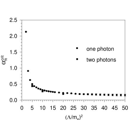
FIG. 6.: The critical coupling $\alpha_{R}^{\rm crit}$ as a function of cutoff $\Lambda$. This is the upper limit of the range allowed for the physical coupling; beyond this value there is no solution for the bare coupling, as a consequence of the truncations of the theory. The one-photon values are obtained from extrapolations using $\alpha_{R}^{\rm crit}+a_{1}/K+a_{2}/K^{2}+b_{1}/N_{\perp}+b_{2}/N_{\perp}^{2}+c_{11}/(KN_{\perp})$; the error bars represent the difference between this fit and one without the $b_{1}/N_{\perp}$ term. The two-photon values come from a fit to $\alpha_{R}^{\rm crit}+a_{1}/K+a_{2}/K^{2}+b_{1}/N_{\perp}+b_{2}/N_{\perp}^{2}$; the error bars are obtained from a fit without the quadratic terms. For all the photon mass is $m_{\gamma}=m_{e}/10$.

C Infrared singularities

A nonzero photon mass $m_{\gamma}$ is used to eliminate the usual infrared singularities. Because the calculation deals with a charged system, there would otherwise be considerable difficulty with soft photons[68]. On the light cone, there are other singularities not removed by the photon mass. They are associated with contributions that involve zero longitudinal momentum.

The fundamental four-point vertices can be infrared singular, in the limit of zero longitudinal momentum for the instantaneous fermion. They must be allowed to cancel against iterations of the three-point vertices which are also singular. This constrains the bare couplings in the four-point vertices to forms derived from the three-point coupling $e_{0}$. The pairs of diagrams are shown in Fig. 7. The first pair does not actually involve a singularity; however, we do match the four-point coupling to the iterated three-point coupling. The second requires basis states with two photons, which are available in the calculation. The third pair requires the presence of electron-positron pairs in the basis, or an effective interaction in the Hamiltonian. Neither is included at present, and therefore this piece of the instantaneous interaction must also be excluded from the Hamiltonian. Detection of $k^{+}<0$ in the instantaneous interaction can be easily done to exclude this graph.

FIG. 7.: Instantaneous fermion interactions paired with corresponding iterated three-point interactions. The vertical dashed lines indicate the intermediate states of the iterated interactions. In (b) the longitudinal momentum of the instantaneous fermion is positive, and in (c) it is negative; this represents a separation of the crossed-photon graph into two pieces.

Other infrared singularities are associated with the emission and absorption of real photons with longitudinal momentum near zero[69]. In perturbative calculations these are regulated by the Mandelstam–Leibbrandt prescription[70]. Viewed in $x^{+}$-ordered perturbation theory, each intermediate state contributes a denominator in which the light-cone energy $k^{-}=(m_{\gamma}^{2}+k_{\perp}^{2})/k^{+}$ of the photon becomes large, and each vertex can contain a factor of $(k^{+})^{-3/2}$. If $k^{+}$ is separately regulated, with some lower cutoff $\epsilon$, graphs with multiple photons will contribute powers of $\log\epsilon$ or even $\epsilon^{-1}$. For a Tamm-Dancoff approximation to a charged system, these cannot be expected to cancel. The choice of the invariant mass cutoff (11) instead couples the regulation of small $k^{+}$ to that of large $k_{\perp}$. The combination prevents the small $k^{+}$ region of integration from making large contributions except in cases where there are already ultraviolet transverse divergences. These spurious infrared infinities are then handled by the mass and coupling renormalization discussed in this section.

D Four-point graphs

There remains a logarithmic divergence associated with four-point graphs of the sort illustrated in Fig. 8(a) and (b). If all graphs of this order are included in a perturbative calculation, the logarithms cancel. However, the Tamm-Dancoff truncation of the present calculation excludes some graphs, such as the one shown in Fig. 8(c), and the cancellation can no longer take place. In a nonperturbative calculation one must include the equivalent of diagrams with an arbitrary number of interlocked loops, such as Fig. 8(b), which are also logarithmically divergent. The needed counterterm is of the form $\lambda(p_{i}^{+},p_{f}^{+})\log\Lambda$ but cannot be found analytically without summing all the infinite chains of interlocked loops.

FIG. 8.: Logarithmically divergent four-point graphs. Those with no more than two photons in any intermediate state, (a) and (b), are included in the present calculation. The nonperturbative nature of the calculation implies that (b) can have an arbitrary number of loops. Diagram (c), which contains three photons in flight is not included.

One way to approach the construction of $\lambda(p_{i}^{+},p_{f}^{+})$ is to fit Compton amplitudes to data[7]. This will require development of techniques to describe scattering processes within DLCQ. A generalization of earlier work[45, 71] on the inversion of the full Greens function may be useful as a means for computing the $T$ matrix and thus scattering amplitudes. We do not consider this further here. The results presented in Sec. V do still contain the $\log\Lambda$ divergence.

IV Finite corrections

A Photon zero modes

As applied to QED, DLCQ requires the use of periodic boundary conditions for the photon field. This is because photons couple to fermion bilinears, which are automatically periodic, even if the preferred antiperiodic boundary conditions are used for the fermions. For fields periodic in the longitudinal direction $x^{-}$, there are contributions from zero modes[26, 57, 58, 59, 60], modes independent of $x^{-}$ that correspond to zero longitudinal momentum. As shown by Pauli and Kalloniatis[57], these modes prevent the choice of ordinary light-cone gauge because the zero-mode piece of $A^{+}$ cannot be gauged away. Instead this piece must satisfy a constraint equation. In fact, careful application of DLCQ to most bosonic theories will result in constraint equations that relate the zero-mode contribution to the normal-mode operators in a nonlinear, nontrivial way. For QED there are zero modes in all the components of the photon field, for which constraint equations must be solved. What is more, the constraint equation for the dependent piece of the fermion field, which is easily solved in light-cone gauge in the continuum, becomes coupled to the zero-mode constraint equations. A formulation of the coupled system of constraints has been given by Kalloniatis and Robertson[56]. Extension of these constraints to include a nonzero photon mass is straightforward.

The constraint equations are difficult to solve, even in simpler theories[60]. This is partly because they couple states with different $P^{+}$ and require study of convergence as a function of some $P^{+}$ cutoff. The difficulty is also due to the need for an ultraviolet cutoff and renormalization of masses and couplings. Because the renormalization is formulated in terms of solutions to the mass eigenvalue problem and because the Hamiltonian cannot be formed until the zero-mode contribution is known, the problem expands to a very large nonlinear system of simultaneous equations. As a result of these difficulties, the calculations discussed here do not include zero modes. However, some progress has been made recently by Kalloniatis[72] in the solution of constraint equations for SU(2) Yang-Mills in $1+1$ dimensions coupled to massive adjoint scalars.

For theories such as QED where symmetry breaking effects are not expected, solution of constraint equations may not be necessary. One can instead treat the end-point behavior of photon amplitudes in a manner similar to that of the “ladder relations” studied by Antonuccio and Dalley[40]. Behavior of amplitudes at small longitudinal momentum, as extracted from the integral equations, can be used to construct effective interactions that include zero modes to leading order in $1/K$. This is equivalent to the approach used in[35] where the behavior of the exchange kernel was studied in a scalar theory to determine the effective interaction[73]. To keep zero-mode terms to higher order in $1/K$ would actually be inconsistent with DLCQ’s neglect of higher order non-zero-mode terms. In the work of Ref. [35] inclusion of the zero-mode contributions ${\cal O}(1/K)$ did improve convergence.

The whole issue may actually be moot when the invariant mass cutoff (11) is used. This cutoff explicitly excludes contributions from states with zero longitudinal momentum. The meaning of this exclusion for nondynamical fields is unclear. The calculations that showed zero modes to be useful for convergence[35] did not employ the invariant mass cutoff. New calculations need to be carried out specifically to study the effect of cutoff choice on the importance of zero modes.

B Restoration of symmetries

The use of light-cone coordinates, combined with the Tamm-Dancoff truncation in particle number and the invariant mass cutoff, explicitly break symmetries of the theory[10]. In particular, rotational symmetry about the transverse axes is broken because the associated operators involve the interaction and therefore change particle number. The change in particle number cannot be accommodated in field theory without allowing an infinite number of particles.

Restoration of such symmetries can be accomplished by the addition of finite counter-terms to the Hamiltonian[74, 75] including adjustment of the “vertex mass,” which appears in the spin-flip vertex, relative to the “kinetic mass”[74]. The ambiguities associated with the infinite counterterms allow such finite terms to exist[10]. Restoration of symmetries is then viewed as a source of conditions by which these finite parts can be determined. In practice, this might involve study of processes[76] such as Compton scattering[7] or electron-electron scattering.

Given the Tamm-Dancoff truncation, an alternative is to view the eigenvalue problem as a few-body problem[77] for which the correct effective Hamiltonian and the generators of translations, rotations, and boosts must satisfy the usual Poincaré algebra[78]. The effective operators might be constructed by adding minimal finite corrections to their field-theoretic forms. The finite corrections are determined by the requirement that the Poincaré algebra be satisfied.

For the results presented here, no attempt has been made to include these finite corrections.

V Results

An accurate DLCQ calculation for a basis with at most one photon can be easily done when instantaneous interactions are neglected. The accuracy can be verified directly because the integrals that yield $a_{e}$ can be performed analytically[20]. In the limit of infinite cutoff and zero photon mass this reproduces the Schwinger[18] result of $\alpha_{R}/2\pi$. The only coupling renormalization is a trivial wave function renormalization. The DLCQ result at various cutoff values is shown in Fig. 9 for a photon mass of $m_{e}/10$. Weighting methods[17] are a critical part of the calculation.

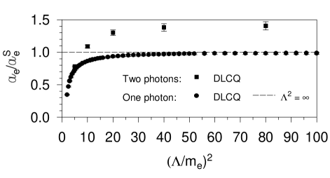
FIG. 9.: The ratio of the renormalized anomalous moment $a_{e}$ to the exact one-photon perturbative result $a_{e}^{S}$ at the same photon mass $m_{\gamma}$, as a function of the invariant-mass cutoff $\Lambda$. Here $m_{\gamma}=m_{e}/10$, and $\alpha_{R}=0.1$. The Fock space is truncated to include at most one or two photons. The DLCQ results are extrapolated from calculations done with $K=21$ to 31, and $N_{\perp}=8$ to 15 for one photon and $N_{\perp}=7$ to 9, 10, or 11 for two photons.

Calculations with a basis that includes at most two photons have been done at five different values of the cutoff for a coupling of $\alpha_{R}=0.1$. They are also shown in Fig. 9. The two-photon contribution adds approximately 40%. This is much larger than the order of magnitude ($\alpha/\pi$ or 3%) that one would expect. It is also opposite in sign to the Sommerfield–Petermann contribution[79] of $-0.328(\alpha/\pi)^{2}$ to the anomalous moment. We attribute this large difference to the absence of Z graphs.

The basis sizes involved are on the order of 1 to 4 million, which translates to solution of linear systems with 4000 to 10,000 variables once the two-photon states are integrated out and symmetries of the one-photon states are used.

The values obtained from DLCQ were extrapolated to $K=\infty$ and $N_{\perp}=\infty$ by fits to $a_{e}+a/K+b/N_{\perp}+c/(KN_{\perp})$. Exclusion of the last term provided an estimate of the error in the fit, which is reflected in the error bars in Fig. 9. The values of $K$ ranged from 21 to 31 and those of $N_{\perp}$ from 7 to 9, 10 or 11, depending on matrix size limitations.

The time required for an extrapolated value at a fixed cutoff is roughly 10 hours on a Cray X-MP, using less than 32 million words of memory. This seems quite competitive with older lattice methods, where a quenched QCD calculation of heavy-light meson wave functions[80] required 300 hours on a CM-200[81], but does not yet match the effort required with the latest methods[51], for which calculation of the B meson magnetic form factor might require 50 hours on a good PC[82].

VI Summary

The nonperturbative calculation of the anomalous moment of the electron $a_{e}$, besides being of intrinsic interest itself, exposes many important issues for nonperturbative calculations within gauge theories which occur in the context of a truncated Fock space. These include nonperturbative mass and coupling renormalization, control of spurious infrared singularities, determination of zero-mode contributions, and the construction of finite counterterms which restore symmetries. Each of these has been addressed in the preceding sections, and the first two have been incorporated into a DLCQ calculation where as many as two photons are included in the basis.

We have presented results for $a_{e}$ computed in a light-cone-gauge Fock space truncated to include one bare electron and at most two photons; i.e., up to two photons in flight. The calculational scheme uses an invariant mass cutoff, discretized light-cone quantization (DLCQ), a Tamm–Dancoff truncation of the Fock space, and a photon mass regulator. We have utilized new weighting methods which greatly improve convergence to the continuum within DLCQ. A large renormalized coupling strength $\alpha_{R}=0.1$ is then used to make the nonperturbative effects in the electron anomalous moment from the one-electron, two-photon Fock state sector numerically detectable. Results are given in Fig. 9.

The disagreement between these results and what one would expect from perturbation theory at order $\alpha^{2}$ indicates that the effect of Z graphs needs to be included in a systematic way. This can be done as an effective interaction, to avoid expansion of the Fock basis to include pair states. The corresponding piece of the instantaneous fermion interaction, as depicted in Fig. 7(c), must then also be included to maintain an infrared cancellation.

Further progress in computing the electron moment will require:

1. New counterterms: One piece of the infinite renormalization is missing in the calculation. As discussed in Section III D, it requires a new nonperturbative counterterm for the logarithmic divergences present in diagrams of the type shown in Fig. 8(a) and (b). The divergence arises because the Tamm–Dancoff truncation prevents certain cancellations. Construction of the counterterm will likely require analysis of scattering processes.

2. Zero modes in DLCQ: Before full consideration of photon zero modes is undertaken, we recommend renewed study of zero modes in a scalar theory where the constraint equation can be solved exactly[35]. This may show that, when the invariant mass cutoff (11) is used, zero modes do not make a significant numerical contribution. If instead there is an important contribution, it should be computed only to leading order in the numerical resolution, to be consistent with the level of approximation used in the basic DLCQ approach.

3. Use of symmetries in DLCQ renormalization: The restoration of symmetries should then complete construction of the light-cone Hamiltonian. One can normalize to specific physical processes[76, 7] or take an abstract approach based on the algebra of the Poincaré generators[77, 78].

4. Higher Fock States: Once the two-photon calculation is fully under control, the addition of $eee^{+}$ states can be considered. This will require analysis of photon mass and wave function renormalization.

Many of the complications of the light-cone Fock state analysis presented here can be traced to the complexity of sector-dependent renormalization. Given such complications the newly developed alternative of Pauli–Villars regularization[17] may be the preferred approach. Within such a scheme, it is also likely that the limitation to a small number of photons can be relaxed.

The analysis presented here is the first step in a systematic program to compute physical quantities in gauge theory systematically utilizing a light-cone Fock expansion. It will also be interesting to use these methods and the present knowledge of the dressed-electron state in QED in order to systematically construct the neutral positronium state as a composite of a dressed electron and positron. Such an analysis can serve as the prototype for systemic nonperturbative construction of colorless bound state hadrons in QCD.

REFERENCES

• [1] R.P. Feynman, in The Quantum Theory of Fields, (Interscience, New York, 1961).
• [2] S.D. Drell and H.R. Pagels, Phys. Rev. 140, B397 (1965).
• [3] W. Thirring, Phil. Mag. 41, 1193 (1950); F. Low, Phys. Rev. 96, 1428 (1954); M. Gell-Mann and M. Goldberger, Phys. Rev. 96, 1433 (1954).
• [4] P.A.M. Dirac, Rev. Mod. Phys. 21, 392 (1949); for an alternate approach in terms of the infinite-momentum frame, see S. Weinberg, Phys. Rev. 150, 1313 (1966).
• [5] For reviews and discussion, see G.P. Lepage and S.J. Brodsky, Phys. Rev. D 22, 2157 (1980); S.J. Brodsky, T. Huang, and G.P. Lepage in Springer Tracts in Modern Physics Vol. 100 (Springer–Verlag, Berlin, 1982); G.P. Lepage, S.J. Brodsky, T. Huang, and P.B. MacKenzie, in proceedings of the 1981 Banff Summer Institute on Particle Physics, Alberta, Canada; J.M. Namyslowski, Prog. in Part. and Nucl. Phys. 14, 49 (1985); S.J. Brodsky and H.-C. Pauli, in Recent Aspects of Quantum Fields, edited by H. Mitter and H. Gausterer, Lecture Notes in Physics Vol. 396 (Springer–Verlag, Berlin, 1991); S.J. Brodsky, G. McCartor, H.-C. Pauli, and S.S. Pinsky, Part. World 3, 109 (1993); K.G. Wilson, T.S. Walhout, A. Harindranath, W.-M. Zhang, R.J. Perry, and St.D. Głazek, Phys. Rev. D 49, 6720 (1994); T. Heinzl and E. Werner, Z. Phys. C 62, 521 (1994); S.J. Brodsky and D.G. Robertson, in the proceedings of the 1995 ELFE Summer School and Workshop, Confinement Physics, edited by S. Bass and P.A.M. Guichon, (Gif-sur-Yvette, Ed. Frontieres, 1996), p. 71; M. Burkardt, Adv. Nucl. Phys. 23, 1 (1996); S.J. Brodsky, H.-C. Pauli, and S.S. Pinsky, SLAC-PUB-7484, submitted to Phys. Rep., Report No. hep-ph/9705477 (unpublished).
• [6] H.-C. Pauli and S.J. Brodsky, Phys. Rev. D 32, 1993 (1985); 32, 2001 (1985).
• [7] D.Mustaki and S. Pinsky, Phys. Rev. D 45, 3775 (1992).
• [8] J.R. Hiller, in the proceedings of the workshop Theory of Hadrons and Light-Front QCD, Zakopane, Poland, August 16-25, 1994, edited by St.D. Głazek, (World Scientific, Singapore, 1995), p. 277; J.R. Hiller and S.J. Brodsky, in The Minneapolis Meeting (DPF96): Proceedings of the 1996 Meeting of the American Physical Society Division of Particles and Fields, edited by K. Heller, J.K. Nelson, and D. Reeder, (World Scientific, Singapore, 1998), Vol. I, p. 619, hep-ph/9608493; J.R. Hiller, in the proceedings of Orbis Scientiae 1997, High-Energy Physics and Cosmology: Celebrating the Impact of 25 Coral Gables Conferences, (Plenum, New York, 1998), in press, Report No. hep-ph/9703451.
• [9] I. Tamm, J. Phys. (Moscow) 9, 449 (1945); S.M. Dancoff, Phys. Rev. 78, 382 (1950).
• [10] R.J. Perry, A. Harindranath, and K.G. Wilson, Phys. Rev. Lett. 65, 2959 (1990); R.J. Perry and A. Harindranath, Phys. Rev. D 43, 4051 (1991); K.G. Wilson et al., Ref. VI.
• [11] R.J. Perry and K.G. Wilson, Nucl. Phys. B403, 587 (1993); R.J. Perry, Ann. Phys. (NY) 232, 116 (1994); R.J. Perry, lectures presented at Hadrons 94, Gramado, Brasil, April 1994; E.A. Ammons, Phys. Rev. D 50, 980 (1994); 54, 5153 (1996); T. Sugihara and M. Yahiro, ibid53, 7239 (1996); 55, 2218 (1997).
• [12] For related work on model theories, see St.D. Głazek and R. J. Perry, Phys. Rev. D 45, 3734 (1992); 45, 3740 (1992); M. Brisudová and St.D. Głazek, ibid50, 971 (1994).
• [13] K.G. Wilson et al., Ref. VI; St.D. Głazek and K.G. Wilson, Phys. Rev. D 48, 5863 (1993); 49, 4214 (1994); T. Masłowski and M. Wiȩckowski, Phys. Rev. D 57, 4976 (1998); St.D. Głazek, Report No. hep-th/9706212 (unpublished); Report No. hep-th/9707028 (unpublished); Report No. hep-th/9712188 (unpublished).
• [14] F. Wegner, Ann. der Physik 3, 77 (1994); E.L. Gubankova and F. Wegner, Report No. hep-th/9702162 (unpublished); Report No. hep-th/9710233 (unpublished); Report No. hep-th/9801018 (unpublished).
• [15] M. Brisudová and R.J. Perry, Phys. Rev. D 54, 1831 (1996); M. Brisudová and R.J. Perry, ibid54, 6453 (1996); M. Brisudová, R.J. Perry, and K.G. Wilson, Phys. Rev. Lett. 78, 1227 (1997); B.D. Jones, R.J. Perry, and St.D. Głazek, Phys. Rev. D 55, 6561 (1997); B.D. Jones and R.J. Perry, ibid., 7715 (1997); M.M. Brisudová, S. Szpigel, and R.J. Perry, Report No. hep-ph/9709479 (unpublished). See also K. Harada and A. Okazaki, ibid., 6198 (1997).
• [16] W. Pauli and F. Villars, Rev. Mod. Phys. 21, 4334 (1949).
• [17] S.J. Brodsky, J.R. Hiller, and G. McCartor, Report No. hep-th/9802020, Phys. Rev. D, to appear, 1998.
• [18] J. Schwinger, Phys. Rev. 73, 416 (1948); 76, 790 (1949).
• [19] For perturbative DLCQ calculations of the electron’s anomalous moment, see A. Langnau, Ph.D. thesis, SLAC Report 385, 1992; A. Langnau and S.J. Brodsky, J. Comput. Phys. 109, 84 (1993); A. Langnau and M. Burkardt, Phys. Rev. D 47, 3452 (1993).
• [20] S.J. Brodsky and S.D. Drell, Phys. Rev. D 22, 2236 (1980). For discussion of renormalization issues, see S.J. Brodsky, R. Roskies, and R. Suaya, Ref. VI.
• [21] A.C. Tang, Ph.D. thesis, SLAC Report No. 351, 1990; A.C. Tang, S.J. Brodsky, and H.-C. Pauli, Phys. Rev. D 44, 1842 (1991).
• [22] T. Kinoshita, Phys. Rev. Lett. 75, 4728 (1995); S. Laporta and E. Remiddi, Phys. Lett. B 379, 283 (1996). For Padé-improved predictions, see J. Ellis, M. Karliner, M.A. Samuel, and E. Steinfelds, SLAC-PUB-6670, Report No. hep-ph/9409376 (unpublished).
• [23] D. Mustaki, S. Pinsky, J. Shigemitsu, and K.G. Wilson, Ref. VI.
• [24] E.V. Prokhvatilov and V.A. Franke, Sov. J. Nucl. Phys. 49, 688 (1989); F. Lenz, M. Thies, S. Levit, and K. Yazaki, Ann. Phys. (N.Y.) 208, 1 (1991); K. Hornbostel, Phys. Rev. D 45, 3781 (1992); E.V. Prokhvatilov, H.W.L. Naus, and H.J. Pirner, ibid51, 2933 (1995); J.P. Vary, T.J. Fields, and H.J. Pirner, ibid53, 7231 (1996); H.W.L. Naus, H.J. Pirner, T.J. Fields, and J.P. Vary, ibid56, 8062 (1997).
• [25] For a possible connection between DLCQ and M(atrix) theory, see T. Banks, W. Fischler, S.H. Shenker, and L. Susskind, Phys. Rev. D 55, 5112 (1997); L. Susskind, Report No. hep-th/9704080 (unpublished); L. Motl and L. Susskind, Report No. hep-th/9708083 (unpublished); F. Antonuccio, H.-C. Pauli, and S. Tsujimaru, Report No. hep-th/9707146 (unpublished).
• [26] A. Harindranath and J.P. Vary, Phys. Rev. D 36, 1141 (1987); 37, 1064 (1988); 37, 1076 (1988); 37, 3010 (1988).
• [27] T. Eller, H.-C. Pauli, and S.J. Brodsky, Phys. Rev. D 35, 1493 (1987); T. Eller and H.-C. Pauli, Z. Phys. C 42, 59 (1989); J.R. Hiller, Phys. Rev. D 43, 2418 (1991). See also D. Mustaki, Phys. Rev. D 42, 1184 (1990); G. McCartor, Z. Phys. C 52, 611 (1991); 64, 349 (1994); Th. Heinzl, St. Krusche, and E. Werner, Phys. Lett. B256, 55 (1991); B275, 410 (1992); C.M. Yung and C.J. Hamer, Phys. Rev. D 44, 2598 (1991); B. van de Sande, Phys. Rev. D 54, 6347 (1996).
• [28] K. Hornsbostel, Ph.D. thesis, SLAC Report No. 333, 1988; M. Burkardt, Nucl. Phys. A504, 762 (1989); K. Hornbostel, S.J. Brodsky, and H.-C. Pauli, Phys. Rev. D 41, 3814 (1990); T. Sugihara, M. Matsuzaki, and M. Yahiro, ibid50, 5274 (1994); M. Heyssler and A.C. Kalloniatis, Phys. Lett. B354, 453 (1995).
• [29] Y. Ma and J.R. Hiller, J. Comput. Phys. 82, 229 (1989); Y. Mo and R.J. Perry, ibid108, 159 (1993); K. Harada, T. Sugihara, and M. Taniguchi, Phys. Rev. D 49, 4226 (1994); K. Harada, A. Okazaki, and M. Taniguchi, ibid52, 2429 (1995); 54, 7656 (1996); K. Harada, T. Heinzl, and C. Stern, ibid57, 2460 (1998).
• [30] A. Harindranath, R.J. Perry, and J. Shigemitsu, Phys. Rev. D 46, 4580 (1992).
• [31] S. Dalley and I.R. Klebanov, Phys. Rev. D 47, 2517 (1993); G. Bhanot, K. Demeterfi, and I.R. Klebanov, ibid48, 4980 (1993).
• [32] J.R. Hiller, Phys. Rev. D 44, 2504 (1991); J.B. Swenson and J.R. Hiller, ibid48, 1774 (1993); S.H. Ghosh, ibid46, 5497 (1992); 49, 2997 (1994).
• [33] M. Thies and K. Ohta, Phys. Rev. D 48, 5883 (1993); I. Pesando, Mod. Phys. Lett. A10, 525 (1995); A. Ogura, T. Tomachi, and T. Fujita, Ann. Phys. (NY) 237, 12 (1995); Y. Kim, S. Tsujimaru, and K. Yamawaki, Phys. Rev. Lett. 74, 4771 (1995); S. Maedan, Phys. Lett. B 370, 116 (1996).
• [34] M. Sawicki, Phys. Rev. D 32, 2666 (1985); 33, 1103 (1986); M. Sawicki and L. Mankiewicz, ibid37, 421 (1988); 40, 3415 (1989); St.D. Głazek and M. Sawicki, ibid41, 2563 (1990) C.-R. Ji and R.J. Furnstahl, Phys. Lett. 167B, 11 (1986); C.-R. Ji, ibid167B, 16 (1986); C.-R. Ji, Phys. Lett. B322, 389 (1994).
• [35] J.J. Wivoda and J.R. Hiller, Phys. Rev. D 47, 4647 (1993).
• [36] St. Głazek, A. Harindranath, S. Pinsky, J. Shigemitsu, and K. Wilson, Phys. Rev. D 47, 1599 (1993); P.M. Wort, ibid47, 608 (1993).
• [37] M. Kaluža and H.-C. Pauli, Phys. Rev. D 45, 2968 (1992); M. Krautgärtner, H.C. Pauli, and F. Wölz, ibid45, 3755 (1992); M. Kaluža and H.J. Pirner, ibid47, 1620 (1993); H.C. Pauli and J. Merkel, ibid55, 2486 (1997); U. Trittmann and H.-C. Pauli, Report No. hep-th/9704215 (unpublished); Report No. hep-th/9705021 (unpublished); U. Trittmann, Report No. hep-th/9705072 (unpublished); Report No. hep-th/9706055 (unpublished). See also D. Klabucar and H.-C. Pauli, Z. Phys. C 47, 141 (1990).
• [38] L.C.L. Hollenberg, K. Higashijima, R.C. Warner and B.H.J. McKellar, Prog. Th. Phys. 87, 441 (1992). For an equal-time approach, see J.R. Spence and J.P. Vary, Phys. Rev. C 52, 1668 (1995).
• [39] H.-C. Pauli and R. Bayer, Phys. Rev. D 53, 939 (1996).
• [40] F. Antonuccio and S. Dalley, Phys. Lett. B 376, 154 (1996); Nucl. Phys. B 461, 275 (1996); F. Antonuccio and S.S. Pinsky, Phys. Lett. B 397, 42 (1997); F. Antonuccio, Report No. hep-th/9705045 (unpublished); F. Antonuccio, S.J. Brodsky, and S. Dalley, Phys. Lett. B 412, 104 (1997).
• [41] B. van de Sande and M. Burkardt, Phys. Rev. D 53, 4628 (1996); M. Burkardt, ibid56, 7105 (1997).
• [42] G.C. Wick, Phys. Rev. 96, 1124 (1954); R.E. Cutkosky, ibid96, 1135 (1954); E. Zur Linden and H. Mitter, Nuovo Cim. 61B, 389 (1969); G. Feldman, T. Fulton, and J. Townsend, Phys. Rev. D 7, 1814 (1973); L. Muller, Nuovo Cim. 75A, 39 (1983).
• [43] H. Kröger, R. Girard, and G. Dufour, Phys. Rev. D 35, 3944 (1987); R. Girard and H. Kröger, Z. Phys. C 37, 365 (1988); H. Kröger, in the proceedings of the workshop on Relativistic Nuclear Many-Body Physics, edited by B.C. Clark, R.J. Perry, and J.P. Vary (World Scientific, Singapore, 1989), p. 47; J.F. Briere and H. Kröger, Phys. Rev. D 41, 3197 (1990); H. Kröger, Phys. Rep. 210, 45 (1992); A.M. Chaara et al., Phys. Lett. B336, 567 (1994). These include work in both light-cone quantization and equal-time quantization.
• [44] For few-body scattering calculations, see C.-R. Ji and Y. Surya, Phys. Rev. D 46, 3565 (1992); C.-R. Ji, C.-H. Kim, and D.-P. Min, ibid51, 879 (1995).
• [45] J.R. Hiller, Ref. VI.
• [46] H. Kröger and H.-C. Pauli, Phys. Lett. B319, 163 (1993).
• [47] For reviews, see M. Creutz, L. Jacobs and C. Rebbi, Phys. Rep. 93, 201 (1983); J.B. Kogut, Rev. Mod. Phys. 55, 775 (1983); I. Montvay, ibid59, 263 (1987); A.S. Kronfeld and P.B. Mackenzie, Ann. Rev. Nucl. Part. Sci. 43, 793 (1993); J.W. Negele, Nucl. Phys. A553, 47c (1993). For predictions of hadron masses, see F. Butler et al., Phys. Rev. Lett. 70, 2849 (1993).
• [48] For discussions of nonperturbative renormalization in lattice calculations, see K. Jansen et al., Phys. Lett. B 372, 275 (1996) and references therein.
• [49] L. Reinders, H. Rubinstein, and S. Yazaki, Phys. Rep. 127, 1 (1985); Vacuum Structure and QCD Sum Rules, M. Shifman, ed. (North Holland, Amsterdam, 1992).
• [50] C.D. Roberts and A.G. Williams, Prog. Part. Nucl. Phys. 33, 477 (1994).
• [51] M. Alford, W. Dimm, G.P. Lepage, G. Hockney, and P.B. Mackenzie, Phys. Lett. B361, 87 (1995) and references given therein.
• [52] J.B. Kogut and L. Susskind, Phys. Rev. D 11, 395 (1975).
• [53] See, for example, J.B. Bronzan and Y. Günal, Phys. Rev. D 50, 5924 (1994); L.C.L. Hollenberg, M.P. Wilson, and N.S. Witte, Phys. Lett. B361, 81 (1995); and references given therein.
• [54] W.A. Bardeen and R. Pearson, Phys. Rev. D 14, 547 (1976); W.A. Bardeen, R.B. Pearson, and E. Rabinovici, ibid21, 1037 (1980); P.A. Griffin, Mod. Phys. Lett. A 7, 601 (1992); Nucl. Phys. B372, 270 (1992); Phys. Rev. D 46, 3538 (1992); 47, 3530 (1993); M. Burkardt, ibid47, 4628 (1993); 49, 5446 (1994); M. Burkardt, in the proceedings of the 1995 ELFE Summer School and Workshop, Confinement Physics, edited by S. Bass and P.A.M. Guichon, (Gif-sur-Yvette, Ed. Frontieres, 1996), p. 255; M. Burkardt and B. Klindworth, Phys. Rev. D 55, 1001 (1997).
• [55] C. Destri and H.J. de Vega, Nucl. Phys. B290, 363 (1987); D. Mustaki, Phys. Rev. D 38, 1260 (1989).
• [56] A.C. Kalloniatis and D.G. Robertson, Phys. Rev. D 50, 5262 (1994).
• [57] A.C. Kalloniatis and H.-C. Pauli, Z. Phys. C 60, 255 (1993); 63, 161 (1994). For an extension of this work to QCD, see A. C. Kalloniatis, H.-C. Pauli, and S. Pinsky, Phys. Rev. D 50, 6633 (1994); H.-C. Pauli, A.C. Kalloniatis, and S.S. Pinsky, ibid52, 1176 (1995); M. Tachibana, ibid52, 6008 (1995); S.S. Pinsky and A.C. Kalloniatis, Phys. Lett. B 365, 225 (1996); A.C. Kalloniatis, Phys. Rev. D 54, 2876 (1996); S.S. Pinsky and D.G. Robertson, Phys. Lett. B 379, 169 (1996); R. Mohr and S.S. Pinsky, ibid401, 301 (1997); S.S. Pinsky, Phys. Rev. D 56, 5040 (1997). See also K. Demeterfi, I.R. Klebanov, and G. Bhanot, Nucl. Phys. B 418, 15 (1994); F. Lenz, M. Shifman, and M. Thies, Phys. Rev. D 51, 7060 (1995); A.C. Kalloniatis and D.G. Robertson, Phys. Lett. B 381, 209 (1996); Ľ. Martinovič, Phys. Lett. B 400, 335 (1997). For related work on zero modes and gauge fixing in QED, see F. Lenz, H.W.L. Naus, K. Ohta, and M. Thies, Ann. Phys. (NY) 233, 17 (1994); 233, 51 (1994).
• [58] T. Maskawa and K. Yamawaki, Prog. Theor. Phys. 56, 270 (1976); St.D. Głazek, Phys. Rev. D 38, 3277 (1988); C. Dietmaier, Th. Heinzl, M. Schaden, and E. Werner, Z. Phys. A 334, 215 (1989); Th. Heinzl, St. Krusche, and E. Werner, ibid334, 443 (1989); C.J. Benesh and J.P. Vary, Z. Phys. C 49, 411 (1991); D.G. Robertson and G. McCartor, ibid53, 661 (1992); G.McCartor and D.G. Robertson, ibid53, 679 (1992); K. Hornbostel, Ref. VI; Th. Heinzl, St. Krusche, E. Werner, and B. Zellermann, Universität Regensburg preprint TPR 92-17, 1992; R.W. Brown, J.W. Jun, S.M. Shvartsman, and C.C. Taylor, Phys. Rev. D 48, 5873 (1993); Th. Heinzl and E. Werner, Z. Phys. C 62, 521 (1994); E.V. Prokhvatilov, H.W.L. Naus, and H.-J. Pirner, Phys. Rev. D 51, 2933 (1995); M.E. Convery, C.C. Taylor, and J.W. Jun, ibid51, 4445 (1995); K. Harada, A. Okazaki, and M. Taniguchi, ibid55, 4910 (1997).
• [59] R.S. Wittman, in Nuclear and Particle Physics on the Light Cone, edited by M.B. Johnson and L.S. Kisslinger, (World-Scientific, Singapore, 1989), p. 331; Th. Heinzl, St. Krusche, and E. Werner, Phys. Lett. 272B, 54 (1991); Th. Heinzl, St. Krusche, S. Simburger, and E. Werner, Z. Phys. C 56, 415 (1992); D.G. Robertson, Phys. Rev. D 47, 2549 (1993); A. Borderies, P. Grangé, and E. Werner, Phys. Lett. B319, 490 (1993); B345, 458 (1995); X. Xu and H.J. Weber, Phys. Rev. D 52, 4633 (1995); T. Heinzl, Phys. Lett. B 388, 129 (1996); M. Burkardt and H. El-Khozondar, Phys. Rev. D 55, 6514 (1997).
• [60] C. M. Bender, S. S. Pinsky, and B. van de Sande, Phys. Rev. D 48, 816 (1993); S. S. Pinsky and B. van de Sande, ibid49, 2001 (1994); S.S. Pinsky, B. van de Sande, and J.R. Hiller, ibid51, 726 (1995).
• [61] S.J. Chang and S.-K. Ma, Phys. Rev. 180, 1506 (1969); S.D Drell, D.J. Levi, and T.-M. Yan, Phys. Rev. D 1, 1035 (1970); J.B. Kogut and D.E. Soper, ibid1, 2901 (1970); D.E. Soper, ibid4, 1620 (1971); J.D. Bjorken, J.B. Kogut, and D.E. Soper, ibid3, 1382 (1971); S.-J. Chang, R.G. Root, T.-M. Yan, ibid7, 1133 (1973); S.-J. Chang and T.-M. Yan, ibid7, 1147 (1973); T.-M. Yan, ibid7, 1760 (1973); 7, 1780 (1973); J. Kogut and L. Susskind, Phys. Rep. 8, 75 (1973); S.J. Brodsky, R. Roskies, and R. Suaya, Phys. Rev. D 8, 4574 (1973).
• [62] A. Harindranath and R.J. Perry, Phys. Rev. D 43, 492 (1991); 43, 3580(E) (1991); D. Mustaki, S. Pinsky, J. Shigemitsu, and K.G. Wilson, ibid43, 3411 (1991); R.J. Perry, Phys. Lett. B300, 8 (1993); W.-M. Zhang and A. Harindranath, Phys. Rev. D 48, 4868 (1993); 48, 4881 (1993); 48, 4903 (1993); N.E. Ligterink and B.L.G. Bakker, Phys. Rev. D 52, 5917 (1995); 5954 (1995); N.C.J. Schoonderwoerd and B.L.G. Bakker, Phys. Rev. D 57, 4965 (1998); Report No. hep-ph/9801433 (unpublished).
• [63] S.D. Drell and T.-M. Yan, Phys. Rev. Lett. 24, 181 (1970).
• [64] G.P. Lepage, summary talk, SMU light-cone workshop (1991); St.D. Głazek and K.G. Wilson, Ref. VI.
• [65] V.G. Koures, Phys. Lett. B348, 170 (1995).
• [66] For a discussion of the use of Weyl gauge in DLCQ, see J. Przeszowski, H.W.L. Naus, and A.C. Kalloniatis, Phys. Rev. D 54, 5135 (1996).
• [67] For an alternative approach, see B. van de Sande and S.S. Pinsky, Phys. Rev. D 46, 5479 (1992).
• [68] For a discussion in the context of light-cone quantization, see A. Misra, Phys. Rev. D 50, 4088 (1994).
• [69] A. Casher, Phys. Rev. D 14, 452 (1976).
• [70] S. Mandelstam, Nucl. Phys. B213, 149 (1983); G. Leibbrandt, Phys. Rev. D 29, 1699 (1984); A. Bassetto, G. Nardelli, and R. Soldati, Yang-Mills Theories in Algebraic Noncovariant Gauges, (World-Scientific, Singapore, 1991); A. Basseto, Phys. Rev. D 47, 727 (1993); G. McCartor and D.G. Robertson, Z. Phys. C 62, 349 (1994); 68, 345 (1995). For a nonperturbative application of the prescription, see H.H. Lu and D.E. Soper, Phys. Rev. 48, 1841 (1993).
• [71] R. Haydock, in Solid State Physics, edited by H. Ehrenreich, F. Seitz, and D. Turnbull (Academic, New York, 1980), Vol. 35, p. 283.
• [72] A.C. Kalloniatis, Phys. Rev. D 54, 2876 (1996).
• [73] A first-principles analysis for this scalar theory would be similar to that done for the Yukawa theory in G. McCartor and D.G. Robertson, Ref. VI. For a related discussion of zero modes in a one-dimensional $\phi^{3}$ theory, see M. Maeno, Phys. Lett. B320, 83 (1994).
• [74] M. Burkardt and A. Langnau, Phys. Rev. D 44, 1187 (1991); 44, 3857 (1991); M. Burkardt, ibid54, 2913 (1996); 57, 1136 (1998).
• [75] For discussion of restoration of covariance for the current operator, see B.D. Keister, Phys. Rev. D 49, 1500 (1994); W.-M. Zhang, Phys. Lett. B333, 158 (1994).
• [76] For QCD, the heavy Q$\bar{\rm Q}$ potential is considered in M. Burkardt, Ref. VI.
• [77] H. Leutwyler and J. Stern, Ann. Phys. (NY) 112, 94 (1978); B.L.G. Bakker, L.A. Kondratyuk and M.V. Terent’ev, Nucl. Phys. B158, 497 (1979); B.D. Keister and W.N. Polyzou, in Advances in Nuclear Physics, Vol. 20, edited by J.W. Negele and E. Vogt, (Plenum, New York, 1991), p. 225; M.G. Fuda, Ann. Phys. 231, 1 (1994) and references given therein; M.G. Fuda, Phys. Rev. C 52, 2875 (1995).
• [78] J.B. Kogut and D.E. Soper, Ref. VI.
• [79] C. Sommerfield, Phys. Rev. 107, 328 (1957); A. Petermann, Helv. Phys. Acta. 30, 407 (1957).
• [80] A.A. Khan, C.T.H. Davies, S. Collins, J. Sloan, and J. Shigemitsu, Phys. Rev. D 53, 6433 (1996).
• [81] J. Shigemitsu, private communication.
• [82] G.P. Lepage, private communication.