Abstract

We show that the leading power corrections to the event shape distributions can be resummed into nonperturbative shape functions that do not depend on the center-of-mass energy and measure the energy flow in the final state. In the case of the thrust variable, the distribution is given by the convolution of the perturbative spectrum with the shape function. Choosing the simplest ansatz for the shape function we find that our predictions for the thrust distribution provide a good description of the data in a wide range of energies.

1. Introduction

Study of hadronization corrections to the event shapes in $\mathop{\rm e}\nolimits^{+}\mathop{\rm e}\nolimits^{-}$ annihilation became a unique laboratory for testing QCD dynamics beyond perturbative level [1]. Being infrared and collinear safe quantities, the event shapes (their mean values as well as differential distributions) can be calculated in perturbative QCD at large center-of-mass energies $s\equiv Q^{2}$ as series in $\alpha_{\rm s}(Q)$. Nonperturbative corrections to the event shapes are attributed to hadronization effects and they are expecting to modify perturbative predictions by terms suppressed by powers of large scale $1/Q^{p}$ with the exponent $p$ varying for different observables.

Successful description of the hadronization effects by the phenomenological Monte-Carlo based models indicates that in distinction with the total cross-section of $\mathop{\rm e}\nolimits^{+}\mathop{\rm e}\nolimits^{-}$ annihilation the power corrections to the event shapes become anomalously large and for the shape variables like the thrust and heavy mass jet they are expecting to appear at the level $p=1$.

The enhancement of hadronization corrections occurs due to the fact that the event shapes are not completely inclusive quantities with respect to the final states but rather weighted cross-sections in which large power corrections can be attributed to an incomplete cancellation of the contribution of soft gluons. As a consequence, the operator product expansion (OPE) is not applicable to the analysis of the event shapes and the standard identification of the exponents $p$ characterizing the strength of power corrections as dimensions of local composite operators entering the OPE does not hold.

To determine the leading exponent $p$ and also to understand the way in which nonperturbative effects modify perturbative predictions one may explore instead by now standard infrared renormalon analysis. This procedure has been successfully applied to the mean value of different event shapes variables and the description of the leading $1/Q-$power corrections has been given within different approaches [2]-[7]. In contrast, the hadronization corrections to the differential event shape distributions are less understood. One of the reasons for this is that the leading power corrections to the mean values and to the differential distributions have different form [1]: the former are characterized by a single nonperturbative scale of dimension $p$ while the latter involve the nonperturbative function of the shape variable that one usually estimates running the Monte-Carlo event generators.

Studying the power corrections to the event shape distributions we will follow the approach proposed in [3]. We will mostly concentrate on the differential distribution with respect to the thrust variable $d\sigma/dT$ and, particularly, in the end-point part of the spectrum $T\sim 1$.

There are few reasons for considering the region $T\sim 1$. In contrast with the mean value $\langle{1-T}\rangle$ that gets $1/Q-$power correction from the final states with an arbitrary number of jets, for the thrust distribution in the end-point region, $T\to 1$, one has in the final state only two narrow energetic jets moving close to the light-cone directions $p_{+}$ and $p_{-}$ ($p_{\pm}=\frac{Q}{2}(1,{\bf 0},\pm 1)$ and $2(p_{+}p_{-})=Q^{2}$) in two opposite hemispheres. Denoting their invariant masses as $M_{L}^{2}$ and $M_{R}^{2}$ one gets

$$t\equiv 1-T\simeq\frac{M_{R}^{2}}{Q^{2}}+\frac{M_{L}^{2}}{Q^{2}}\,,$$ (1)

where for later convenience we introduced a new variable $t$.

Taking into account the QCD effects of collinear splitting of quark and gluons inside two narrow jets and their interaction with soft gluon radiation one finds that the thrust distribution for $t\to 0$ depends on two infrared scales, $Q^{2}t^{2}$ and $Q^{2}t$, which give rise to large both perturbative (Sudakov) logs and power corrections. The smallest scale, $(Qt)^{2}$, sets up the total energy carried by soft gluons in the final state and the scale $Q^{2}t$ characterizes the transverse size of the jets $k_{\perp}^{2}={\cal O}(Q^{2}t)$. The power corrections to the thrust distribution are suppressed by powers of both scales. In order to separate the leading asymptotics one keeps the smaller scale $Qt$ fixed and expands the thrust distribution in powers of the larger scale $Q^{2}t$

$$\frac{1}{\sigma_{\rm tot}}\frac{d\sigma}{dt}=\sigma_{0}{\left({\alpha_{\rm s}(Q),\ln t,\frac{1}{Qt}}\right)}+{\cal O}{\left({\frac{1}{Q^{2}t}}\right)}\,.$$ (2)

In what follows we will consider only the leading term of this expansion, $\sigma_{0}$. It should resums large perturbative terms $\alpha_{\rm s}^{n}(Q)\ln^{m}t/t$ ($m\leq 2n-1$) and take into account all power corrections of the form $1/(Qt)^{n}$.

The structure of power corrections $\sim 1/(Qt)^{n}$ strongly depends on the value of the thrust variable. Away from the end-point region, $t\gg\Lambda_{{}_{\rm QCD}}/Q$ one may retain in $\sigma_{0}$ only the lowest term $n=1$ and neglect the terms with $n\geq 2$ as suppressed by powers of $1/Q$. It is this approximation that one applies calculating the mean value of the thrust $\langle{t}\rangle\equiv\sigma_{\rm tot}^{-1}\int_{0}^{t_{\rm max}}dt\,t\frac{d\sigma}{dt}\,,$ where $t_{\rm max}$ is the upper limit on the thrust variable that one imposes to separate the contribution of the 2-jet final state, $t_{\rm max}=\frac{1}{3}$. At the same time, in the end-point region $t={\cal O}(\Lambda_{{}_{\rm QCD}}/Q)$ all terms $\sim(Qt)^{-n}$ become equally important and need to be resummed inside $\sigma_{0}$ for all $n$.

As we will show, the leading power corrections to the thrust distribution in the end-point region away from the small invariant jet mass limit $Q^{2}t\gg\Lambda_{{{}_{\rm QCD}}}^{2}$ can be resummed into a nonperturbative $Q-$independent function that defines the shape of the distribution in the region $t={\cal O}(\Lambda_{{{}_{\rm QCD}}}/Q)$ and therefore is called the shape function. Then, the QCD prediction for the leading term in (2) is given by the convolution of perturbative Sudakov spectrum with nonperturbative shape function. One should mention that one finds similar expressions considering, for example, the large$-x$ asymptotics of the structure function of deep inelastic scattering [8, 9] and the end-point spectrum of the inclusive heavy meson decays $B\to\gamma X_{s}$ [10, 11, 12]. The reason for this similarity is that in all these cases one encounters the same physical situation when energetic narrow jet(s) is propagating in the final state through the cloud of soft gluons. However the important difference with the thrust distribution is that the nonperturbative functions in the latter two cases resum power corrections on the different scale $Q^{2}t$ and they coincide with well-known inclusive (light-cone) distributions.

2. Analysis of soft gluon effects

At the Born level the final state consists of a quark-antiquark pair and the thrust distribution has the form

$$\frac{1}{\sigma_{\rm tot}}\frac{d\sigma}{dt}\bigg{|}_{\rm Born}=\delta(t)\,.$$ (3)

Soft gluon radiation smeares this peak towards larger $t$. Let us first analyze separately perturbative and nonperturbative contributions.

Considering the perturbative emissions of soft gluons out of two outgoing quarks one finds that for $t\to 0$ the phase space for real soft gluons is squeezed and due to an incomplete cancellation between virtual and real gluon contributions the perturbative corrections to the thrust distribution involve large Sudakov logs that can be resummed to all orders with the double logarithmic (DL) accuracy as

$$\frac{1}{\sigma_{\rm tot}}\frac{d\sigma}{dt}\bigg{|}_{\rm PT}=\frac{dR_{{}_{\rm PT}}(t)}{dt}\,,\qquad R_{{}_{\rm PT}}(t)\stackrel{{\scriptstyle\tiny\hbox{\rm DL}}}{{=}}\exp{\left({-\frac{4\alpha_{\rm s}(Q)}{3\pi}\ln^{2}t}\right)}$$ (4)

with $R_{{}_{\rm PT}}(t)$ called the radiator function. One can systematically improve perturbative approximation by including additional nonleading logarithmic terms in $R_{{}_{\rm PT}}(t)$ and matching the result into exact higher order calculations using the $\ln R-$scheme [13]. The perturbative Sudakov spectrum extends over the interval $0\leq t\leq t_{\rm max}$ and vanishes at the end points. The peak of the distribution is located close to $t=0$ and it is shifted towards larger $t$ as one improves perturbative approximation. Its position, $t_{\rm p}={\cal O}(\Lambda_{{}_{\rm QCD}}/Q)$, is sensitive to the emission of soft gluons with energy $\sim\Lambda_{{{}_{\rm QCD}}}$ indicating that the physical spectrum around the peak is of nonperturbative origin.

Let us now estimate the effects of nonperturbative soft gluon emissions on the thrust distribution (3). We take into account that in the leading order in $1/(Q^{2}t)$ the transverse size of two quark jets $k_{\perp}^{2}={\cal O}(Q^{2}t)$ can be neglected, that is soft gluons with the energy $\sim Qt$ can not resolve the internal structure of jets. This means that considering soft gluon emissions we may apply the eikonal approximation and effectively replace quark jets by two relativistic classical particles that carry the color charges of quarks and move apart along the light-cone directions $p_{+}$ and $p_{-}$. The interaction of the quark jets with soft gluons is factorized into the unitary eikonal phase $W(0)$ given by the product of two Wilson lines calculated along classical trajectories of two particles

$$W(0)=W_{+}(0)[W_{-}(0)]^{\dagger}\,,\qquad W_{\pm}(x)=P\exp{\left({i\int_{0}^{\infty}ds\,p_{\pm}\cdot A(x+p_{\pm}s)}\right)}\,,$$ (5)

with gauge fields $A_{\mu}(x)$ describing soft gluons. Denoting the total momentum of soft gluons emitted into the right and left hemispheres as $k_{R}=\sum_{i\in R}k_{i}$ and $k_{L}=\sum_{i\in L}k_{i}$, correspondingly, one finds the thrust (1) as $t=2(k_{R}p_{+})/Q^{2}+2(k_{L}p_{-})/Q^{2}$ and obtains the following expression for the differential distribution

$$\frac{1}{\sigma_{\rm tot}}\frac{d\sigma}{dt}=\sum_{N}\left|\langle 0|W(0)|N\rangle\right|^{2}\delta{\left({t-\frac{k_{R}^{-}}{Q}-\frac{k_{L}^{+}}{Q}}\right)}$$ (6)

with $k^{\pm}=k_{0}\pm k_{3}$. Here, the matrix element of the Wilson line operator describes the interaction of quarks with soft gluons and the summation goes over the final states $N$ of soft gluons with the total momentum $k=k_{R}+k_{L}$. Expression (6) follows from the universality of soft gluon radiation and it takes into account both perturbative and nonperturbative corrections [9].

Let us neglect for the moment the perturbative contribution to the matrix element of the Wilson line in (6). Then, introducing the shape function

$$f(\varepsilon)=\sum_{N}\left|\langle 0|W(0)|N\rangle\right|^{2}\delta{\left({\varepsilon-k_{R}^{-}-k_{L}^{+}}\right)}$$ (7)

one can estimate the nonperturbative contribution to the thrust distribution as

$$\frac{1}{\sigma_{\rm tot}}\frac{d\sigma}{dt}\bigg{|}_{\rm nonPT}=Qf(Qt)\,.$$ (8)

The nonperturbative function $f(\varepsilon)$ is localized at small energies $\varepsilon$ and according to (8) it determines the shape of the spectrum at small $t={\cal O}(\Lambda_{{}_{\rm QCD}}/Q)$.

The important property of the function (7) is that it does not depend on the center-of-mass energy $Q$. Although the vectors $p_{\pm}$ entering into the definition (5) of $W(0)$ do depend on $Q$, the $Q-$dependence of the Wilson lines (5) disappears due to the reparameterization invariance $s\to\lambda s$. Therefore, one may extract the shape function at some reference $Q_{0}$ and then apply it to describe the hadronization effects for different center-of-mass energy.

Being a new nonperturbative distribution, the shape function (7) admits the operator definition that is different however from the one for the inclusive distributions. As a manifestation of noninclusiveness of the thrust variable, $f(\varepsilon)$ depends separately on soft gluon momenta flowing into different hemispheres. In particular, it takes into account the effects of soft gluon splittings when the decay products fly into two different hemispheres [6]. Since this may happen at time scales larger then $1/Q$, we do not expect the function $f(\varepsilon)$ (more precisely its moments) to be related to matrix element of local operators as it happens for inclusive distributions. Indeed, the operator definition of $f(\varepsilon)$ involves the “maximally nonlocal operator” ${\cal E}(\vec{n})$ that measures the density of the energy flow in the direction of unit 3-vector $\vec{n}$. According to its definition ${\cal E}(\vec{n})$ acts on the final state of $N$ particles as ${\cal E}(\vec{n})|{N}\rangle=\sum_{i=1}^{N}k_{i}^{0}\delta(\vec{n}-\vec{k}_{i}/k_{i}^{0})|{N}\rangle$ and it can be expressed in terms of the tensor energy-momentum operator [14, 15]. Then, one uses (7) to get

$$f(\varepsilon)=\langle{0|W^{\dagger}(0)\,\delta{\left({\varepsilon-\int d^{3}n\,(1-|\cos\theta_{\vec{n}}|)\,{\cal E}(\vec{n})}\right)}\,W(0)|0}\rangle\,,$$ (9)

where $\theta_{\vec{n}}$ is the angle between vector $\vec{n}$ and the thrust axis, $\cos\theta_{\vec{n}}=n_{3}$. The detailed properties of this function will be discussed elsewhere [16].

3. Factorization of the thrust distribution

The expression (8) was found by neglecting perturbative soft gluons. It is clear that they also contribute to the matrix element of Wilson lines entering (6) and modify the thrust distribution. In order to combine together perturbative and nonperturbative effects one has to introduce the factorization scale $\mu$ and separate the contribution of soft gluons with the momentum above and below this scale into perturbative Sudakov spectrum, $\frac{d\sigma_{{{}_{\rm PT}}}}{dt}$, and nonperturbative shape function, $f(\varepsilon)$, respectively. Both quantities become functions of the IR cut-off $\mu$ but the thrust distribution is $\mu-$independent.

For the inclusive distributions the above procedure can be performed using the operator product expansion. For the thrust distribution the OPE is not valid and we apply instead the infrared renormalon analysis. To this end we perform perturbative calculation of (6) by summing over the final states $|{N}\rangle$ of multiple perturbative soft gluon radiation and identify the ambiguities of resummed perturbative expressions that can be attributed to nonperturbative contribution. One finds that thanks to the nonabelian exponentiation of the Wilson lines, the perturbative soft gluon contribution exponentiates in the Laplace transform of the distribution [3]

$$\langle{\mathop{\rm e}\nolimits^{-\nu t}}\rangle\equiv\int_{0}^{t_{\rm max}}dt\mathop{\rm e}\nolimits^{-\nu t}\frac{1}{\sigma_{\rm tot}}\frac{d\sigma}{dt}=\exp{\left({-S(\nu)}\right)}$$ (10)

with the leading term in the exponent of the following form

$$S(\nu)=2\int_{0}^{1}\frac{du}{u}{\left({1-\mathop{\rm e}\nolimits^{-u\nu}}\right)}\int_{u^{2}Q^{2}}^{uQ^{2}}\frac{dk_{\perp}^{2}}{k_{\perp}^{2}}\Gamma_{\rm cusp}(\alpha_{\rm s}(k_{\perp}))$$ (11)

and $\Gamma_{\rm cusp}(\alpha_{\rm s})=\frac{4\alpha_{\rm s}}{3\pi}+{\cal O}(\alpha_{\rm s}^{2})$ being a universal cusp anomalous dimension.

We observe that since the singularities of the coupling constant affect the integration over transverse momenta of soft gluons in (11) the Sudakov form factor $S(\nu)$ suffers from infrared renormalon ambiguities. They originate from soft gluons with the energy of order $\Lambda_{\rm QCD}$ whose contribution should be separated into nonperturbative function $f(\varepsilon)$. Namely, introducing the cut-off $\mu$ on the value of transverse gluon momenta in (11) we may split $S(\nu)$ into the sum of two terms. The term with $k_{\perp}^{2}>\mu^{2}$ defines the perturbative contribution to the exponent, $S_{{}_{\rm PT}}(\nu)$, which in turn allows to find the perturbative spectrum $\frac{d\sigma_{{}_{\rm PT}}(t;\mu)}{dt}$ through the inverse Laplace transformation (10). The second term with $k_{\perp}^{2}<\mu^{2}$ should be absorbed into the definition of the nonperturbative function (7). In this case, changing the order of integration in (11) one expands the integral in powers of $\nu$ and absorbs the ambiguous integrals $\int_{0}^{\mu}dk_{\perp}k_{\perp}^{n-1}\Gamma_{\rm cusp}(\alpha_{\rm s}(k_{\perp}))$ into the definition of new nonperturbative scales $\lambda_{n}(\mu)$. Substituting (8) into (10) one finds the following consistency condition

$$\int_{0}^{\infty}d\varepsilon\mathop{\rm e}\nolimits^{-\nu\varepsilon/Q}f(\varepsilon;\mu)=\exp{\left({-\sum_{n=1}^{\infty}\frac{1}{n!}(\nu/Q)^{n}\lambda_{n}(\mu)+{\cal O}(\nu/Q^{2})}\right)}\,.$$ (12)

Although we can not draw any conclusions about the absolute value of the scales $\lambda_{n}$, their $\mu-$dependence is of perturbative origin and it can be determined as

$$\mu\frac{d\lambda_{n}(\mu)}{d\mu}={4(-)^{n+1}}{n^{-1}}\mu^{n}\Gamma_{\rm cusp}(\alpha_{\rm s}(\mu))\,.$$ (13)

Since the parameter $\nu$ is conjugated to the thrust $t$ we neglected in (12) the corrections $\sim\nu/Q^{2}$ and replaced the upper limit of $\varepsilon-$integration, $\varepsilon_{\rm max}=t_{\rm max}Q$, by $\infty$.

The fact that the infrared renormalons contribute additively to the exponent of (10) implies that the Laplace transform of the thrust distribution is factorized into the product of perturbative and nonperturbative terms [3]

$$\langle{\mathop{\rm e}\nolimits^{-\nu t}}\rangle=\langle{\mathop{\rm e}\nolimits^{-\nu t}}\rangle_{{}_{\rm PT}}\times\int_{0}^{\infty}d\varepsilon\mathop{\rm e}\nolimits^{-\nu\varepsilon/Q}f(\varepsilon;\mu)$$ (14)

where $\langle{\mathop{\rm e}\nolimits^{-\nu t}}\rangle_{{}_{\rm PT}}$ is calculated as a mean value with respect to the perturbative distribution $\frac{d\sigma_{{}_{\rm PT}}}{dt}$. Integrating the both sides of this relation with respect to $\nu$ with an appropriate weight we obtain the factorized expression for the radiator function $R(\tau)\equiv\frac{1}{\sigma_{\rm tot}}\int_{0}^{\tau}dt\,\frac{d\sigma}{dt}=\langle{\theta(\tau-t)}\rangle$

$$R(t)=\int_{0}^{tQ}d\varepsilon\,f(\varepsilon;\mu)R_{{}_{\rm PT}}{\left({t-\frac{\varepsilon}{Q};\mu}\right)}\,,$$ (15)

where the upper limit of integration follows from the condition $R_{{}_{\rm PT}}(t)=0$ for $t<0$. Thus, the net effect of incorporating nonperturbative corrections (in the leading $1/(Q^{2}t)-$order) amounts to the $1/Q-$shift of perturbative radiator function smeared with the shape function.

To see how (15) resums both perturbative and nonperturbate corrections, one expands the radiator $R_{{}_{\rm PT}}{\left({t-\frac{\varepsilon}{Q};\mu}\right)}$ in powers of $1/Q$

$$R(t)=R_{{}_{\rm PT}}(t)-\frac{\langle{\varepsilon}\rangle}{Qt}R_{{{}_{\rm PT}}}^{\prime}(t)+\frac{\langle{\varepsilon^{2}}\rangle}{2(Qt)^{2}}[R_{{{}_{\rm PT}}}^{\prime\prime}(t)-R_{{{}_{\rm PT}}}^{\prime}(t)]+\ldots\,,$$ (16)

where prime denotes the logarithmic derivative with respect to $t$. Here, the leading term $R_{{{}_{\rm PT}}}(t)$ gives the resummed perturbative Sudakov expression which is different from (4) due to additional dependence on the IR cut-off $\mu$. The terms with the derivatives of $R_{{{}_{\rm PT}}}$ generate the series of power corrections accompanied by the set of nonperturbative $\mu-$dependent dimensionful parameters $\langle{\varepsilon^{n}}\rangle$ that can be expressed in terms of the scales $\lambda_{k}$ introduced in (12) as

$$\langle{\varepsilon^{n}}\rangle=\int_{0}^{\infty}d\varepsilon\,\varepsilon^{n}f(\varepsilon;\mu)\,,\qquad\langle{\varepsilon}\rangle=\lambda_{1}\,,\quad\langle{\varepsilon}\rangle^{2}-\langle{\varepsilon^{2}}\rangle=\lambda_{2}\,,\quad...$$ (17)

Finally, differentiating the both sides of (15) with respect to $t$ and taking into account that $R_{{{}_{\rm PT}}}(t;\mu)=\theta(t)\int_{0}^{t}dt\frac{d\sigma_{{{}_{\rm PT}}}(t;\mu)}{dt}$ we find the thrust distribution

$$\frac{1}{\sigma_{\rm tot}}\frac{d\sigma(t)}{dt}=Qf(Qt;\mu)R_{{{}_{\rm PT}}}(0;\mu)+\int_{0}^{Qt}d\varepsilon\,f(\varepsilon;\mu)\frac{d\sigma_{{{}_{\rm PT}}}(t-\frac{\varepsilon}{Q};\mu)}{dt}\,.$$ (18)

Here, the two terms in the r.h.s. have the following interpretation. The first term dominates at small $t$ and corresponds to the situation when the perturbative real soft gluon radiation is washed out due to the IR cut-off and the final state consists entirely of nonperturbative radiation described by the shape function. In comparison with (8) one gets the additional Sudakov factor $R_{{{}_{\rm PT}}}(0;\mu)$ that takes into account the perturbative contribution of virtual soft gluons with the energy above the cut-off $\mu$. This factor rapidly vanishes as one decreases the value of $\mu$ allowing more perturbative virtual gluons to be emitted. The second term in (18) describes the smearing of the perturbative Sudakov spectrum by nonperturbative corrections. As an illustration of (18), we depicted on Fig. 1 the contribution of both terms to the thrust distribution at the center-of-mass energy $Q=35\,{\rm GeV}$.

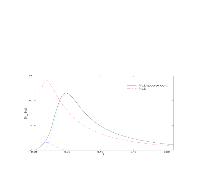
Figure 1: The prediction (18) for the thrust distribution at $Q=35\,{\rm GeV}$. The dotted and dashed lines describe the first and the second term in the r.h.s. of (18), respectively, and the solid line is the sum of both. The dot-dashed line denotes the perturbative Sudakov spectrum $\frac{d\sigma_{{{}_{\rm PT}}}(t;\mu=0)}{dt}$ in the NLL approximation.

In contrast with the heavy meson decay where nonperturbative corrections extend the perturbative spectrum beyond the perturbative end-point due to interaction of the heavy quark in the initial state with the light component of the meson [10, 11], the nonperturbative corrections to the thrust distribution have just an opposite effect. They shift the perturbative spectrum inside the perturbative window $0<t<t_{\rm max}$ and describe an “evaporation” of the energetic jets in the final state due to emission of soft gluons.

4. Nonperturbative ansatz for the shape function

The shape function is a new distribution that resums nonperturbative corrections to the thrust distribution. Although its explicit form can not be extracted from our analysis we could use the renormalon inspired sum rules (12) to study its general properties.

Expanding the both sides of (12) in powers of $1/Q$ we verify that in accordance with its operator definition (9) the function $f(\varepsilon)$ does not depend on the large scale $Q$ and its first few moments are given by (17). The shape function depends on the factorization scale $\mu$ and one may apply the renormalization group equations (13) to find its evolution with $\mu$.

Using (17) one may formally write the shape function in the form of the distribution as a series in $\delta-$function and its derivatives

$$f(\varepsilon;\mu)=\delta(\varepsilon-\lambda_{1})+0\cdot\delta^{\prime}(\varepsilon-\lambda_{1})-\frac{1}{2}\lambda_{2}\delta^{\prime\prime}(\varepsilon-\lambda_{1})+...$$ (19)

Its substitution into (18) yields a series that is equivalent to the expansion of the radiator (16). It is convergent however only for the values of the thrust $\Lambda_{{}_{\rm QCD}}/Q\ll t<t_{\rm max}$ on the tail of the Sudakov spectrum $\frac{d\sigma_{{}_{\rm PT}}}{dt}$ where the perturbative distribution is a slowly varying function of $t$. In this range of $t$, keeping only the first term in the r.h.s. of (19), one finds that the leading power corrections simply renormalize the thrust variable by generating the shift of the perturbative spectrum [3]

$$\frac{1}{\sigma_{\rm tot}}\frac{d\sigma(t)}{dt}=\frac{d\sigma_{{{}_{\rm PT}}}(t-\frac{\langle{\varepsilon}\rangle}{Q})}{dt}\,.$$ (20)

This result is a general property of the leading $1/Q-$power corrections to different event shapes and it is an immediate consequence of the exponentiation of soft gluon contribution. The prediction (20) has been found to be in a good agreement with the data [17].

For the values of the thrust $t={\cal O}(\Lambda_{{}_{\rm QCD}}/Q)$ one needs to know the explicit form of the shape function. In this case, one relies on the particular ansatz for $f(\varepsilon)$ that can be inspired by different model considerations. As the simplest form of $f(\varepsilon)$ we choose the following one

$$f(\varepsilon)={\left({\frac{\varepsilon}{\Lambda}}\right)}^{a-1}\exp{\left({-\frac{\varepsilon^{2}}{\Lambda^{2}}}\right)}\frac{2}{\Lambda\Gamma(\frac{a}{2})}\,.$$ (21)

This function depends on two parameters: dimensionless exponent $a$ controlling how fast the function vanishes at the origin and dimensionfull scale $\Lambda$ defining the interval of energies on which the function is localized. The shape function is peaked around $\varepsilon_{\rm max}=\Lambda\sqrt{\frac{a-1}{2}}$ and it rapidly vanishes for $\varepsilon>\varepsilon_{\rm max}$.

There are additional constraints that we may impose on the shape function. They follow from the analysis of nonperturbative corrections to the mean value of the thrust and its higher moments. Indeed, expanding the both sides of (14) in powers of $\nu$ one gets

$$\langle{t}\rangle=\langle{t}\rangle_{{}_{\rm PT}}+\frac{\langle{\varepsilon}\rangle}{Q}\,,\qquad\langle{t^{2}}\rangle-\langle{t}\rangle^{2}=\langle{t^{2}}\rangle_{{{}_{\rm PT}}}-\langle{t}\rangle^{2}_{{{}_{\rm PT}}}+\frac{\langle{\varepsilon^{2}}\rangle-\langle{\varepsilon}\rangle^{2}}{Q^{2}}\,,\quad...$$ (22)

These relations are valid up to corrections due to contribution to the thrust of the final states with $n\geq 3$ jets. Using (22) and (17) we may relate the parameters of the shape function to the mean value of the first few moments of the thrust. In particular, applying the results of [1] on parameterization of $1/Q-$corrections to the mean value of the thrust we get

$$\langle{t}\rangle-\langle{t}\rangle_{{{}_{\rm PT}}}=\frac{1}{Q}\int_{0}^{\infty}d\varepsilon\,\varepsilon f(\varepsilon)=\frac{0.8\ \rm{GeV}}{Q}$$

Substituting (21) into this relation one still has a freedom in choosing the single parameter $a$ that we define as

$$a=3\,,\qquad\Lambda=0.7\ {\rm GeV}\,.$$ (23)

The shape function corresponding to these values of parameters is shown in Fig. 2. One should stress that the explicit form the shape function (21) as well as the values of the parameters $a$ and $\Lambda$ are related to the particular choice of the factorization scale $\mu$ to be specified later on and they do not depend on the center-of-mass energy $Q$.

Figure 2: The nonperturbative ansatz for shape function.

Let us now consider the perturbative spectrum $\frac{d\sigma_{{{}_{\rm PT}}}(t;\mu)}{dt}$. The contribution of perturbative soft gluons with the energy above the IR cut-off $\mu$ exponentiates in the Laplace transform (10) and $S_{{}_{\rm PT}}(\nu)$ is given by (11) with the additional condition $k_{\perp}^{2}>\mu^{2}$ imposed on the $k_{\perp}-$integration. The important difference with the known results for resummed Sudakov spectrum [13] is in the additional $\mu-$dependence of $\frac{d\sigma_{{{}_{\rm PT}}}(t;\mu)}{dt}$. Nevertheless, one may expand following [13] the exponent $S_{{{}_{\rm PT}}}(\nu)$ in powers of $\alpha_{\rm s}(Q)$ and separate large logarithmic terms $\alpha_{\rm s}^{n}L^{m}$ $(m\leq n+1)$ which due the presence of additional scale appear of two kinds, $L=\ln(Q/\mu)$ and $L=\ln(1/\nu)$. Then, in the NLL approximation that takes into account all terms $\alpha_{\rm s}^{n}L^{n+1}$ and $\alpha_{\rm s}^{n}L^{n}$ in $S_{{{}_{\rm PT}}}(\nu)$ one may replace $1-\mathop{\rm e}\nolimits^{-u\nu}\stackrel{{{}_{\rm NLL}}}{{=}}\theta(u-\mathop{\rm e}\nolimits^{-\gamma_{{}_{\rm E}}}/\nu)$ in (11) and find that due to the condition $k_{\perp}>\mu$ the function $S_{{{}_{\rm PT}}}(\nu)$ has different behaviour depending on the value of $\nu$, or equivalently the thrust $t$. Finally, one performs the inverse Laplace transformation and obtains the radiator function in the NLL approximation as

$$R_{{{}_{\rm PT}}}(t;\mu)\stackrel{{{}_{\rm NLL}}}{{=}}\frac{\exp{\left({-S_{{{}_{\rm PT}}}(t_{0}/t)}\right)}}{\Gamma(1-S_{{{}_{\rm PT}}}^{\prime}(t_{0}/t))}\,,\qquad S_{{{}_{\rm PT}}}^{\prime}(t_{0}/t)=\frac{\partial S_{{{}_{\rm PT}}}(t_{0}/t)}{\partial\ln t}\,,$$ (24)

with $t_{0}=\mathop{\rm e}\nolimits^{\gamma_{{}_{\rm E}}}=1.780...$. Examining this expression one finds that for $t/t_{0}>\mu/Q$ the radiator $R_{{{}_{\rm PT}}}(t;\mu)$ rapidly vanishes at small $t$ and it does not depend on the IR cut-off $\mu$. Thefefore for these values of $t$ it coincides with the known expression from [13]. For $\mu^{2}/Q^{2}<t/t_{0}<\mu/Q$ the radiator $R_{{{}_{\rm PT}}}(t)$ starts to depend on the IR cut-off $\mu$ and, as a consequence, its decrease at small $t$ is slowed down. For $0<t/t_{0}<\mu^{2}/Q^{2}$ the radiator is $t-$independent.

To simplify numerical calculations of the spectrum (18) we ignore the difference between $R_{{{}_{\rm PT}}}(t=t_{0}\mu/Q)$ and $R_{{{}_{\rm PT}}}(t=t_{0}\mu^{2}/Q^{2})$ by choosing the factorization scale $\mu$ to be small but within the applicability range of the NLL approximation [13], $2\beta_{0}\alpha_{\rm s}(Q)\ln(Q/\mu t_{0})<1$. In this case, one may approximate the radiator (24) as

$$R_{{{}_{\rm PT}}}^{\rm app}(t;\mu)=\theta(t/t_{0}-\mu/Q)R_{{{}_{\rm PT}}}(t)+\theta(t)\theta(\mu/Q-t/t_{0})R_{{{}_{\rm PT}}}(\mu/Q)\,,$$ (25)

where $R_{{{}_{\rm PT}}}(t)$ is the known expression for the radiator in the NLL approximation [13] improved by higher order corrections in the $\ln R-$matching scheme. We choose the two free parameters, the factorization scale and the fundamental QCD scale as

$$\mu=0.750\ {\rm GeV}\,,\qquad\Lambda_{{{}_{\rm QCD}}{}_{;}\overline{{}_{\rm MS}}}^{(5)}=0.250\,{\rm GeV}\,.$$

Differentiating the expression (25) with respect to $t$ we obtain the perturbative spectrum $\frac{d\sigma_{{{}_{\rm PT}}}(t;\mu)}{dt}$ that starts at $t=t_{0}\mu/Q$ and extends to $t=t_{\rm max}$.

One should notice that if instead of (25) we would have used for $t/t_{0}\leq\mu/Q$ the expression for the radiator $R_{{{}_{\rm PT}}}(t;\mu)$ in the NLL order, (24), then the perturbative spectrum will have discontinuities at $t/t_{0}=\mu/Q$ and $t/t_{0}=\mu^{2}/Q^{2}$. The reason for this is that $\frac{d\sigma_{{{}_{\rm PT}}}(t;\mu)}{dt}=\frac{R_{{}_{\rm PT}}(t;\mu)}{dt}$ involves the second order derivative of the Sudakov form factor, $S_{{{}_{\rm PT}}}^{\prime\prime}$, that, as it can be seen from (11), is not enhanced by large logarithmic corrections and therefore can not be approximated by the NLL result in the transition regions around these two points.

Finally, let us compare the QCD prediction (18) with available data on the thrust distribution in the interval $0<t<0.33$ at different energies $14<Q/{\rm GeV}<161$. Fig. 3 shows the comparison with the data at $Q=91.2\,{\rm GeV}$, where the most accurate experimental data are available. The combined fit for various center-of-mass energies [18] is shown in Fig. 4. We would like to stress that for different values of $Q$ we use the same ansatz for the shape function, (21), with the parameters defined in (23). As a nontrivial test of (18) we observe that the theoretical curves reproduce well the $Q-$dependence of the data in the end-point region.

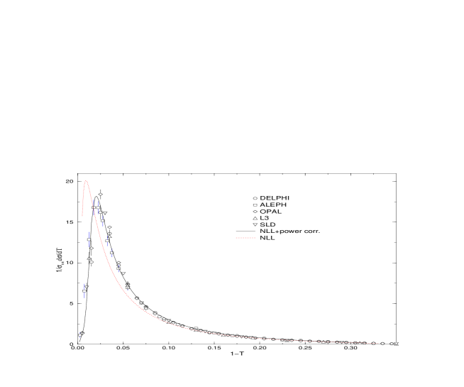
Figure 3: The comparison of the data with the QCD prediction for the thrust distribution (18) at $Q=91.2\,{\rm GeV}$

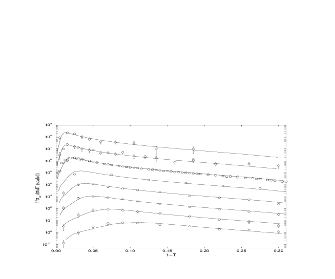
Figure 4: The comparison of the data with the QCD prediction for the thrust distribution at different energies (from bottom to top): $Q/{\rm GeV}=14\,,22\,,35\,,44\,,55\,,91\,,133\,,161.$ [18]

5. Conclusions

We have study the power corrections to the thrust differential distribution in the end-point region of $t$. Due to enhancement of soft gluon contribution, the spectrum is affected by large perturbative Sudakov and nonperturbative $1/(Qt)-$corrections that need to be resummed. Using universal properties of soft gluon radiation we have argued that the resummed leading power corrections are described by the shape function which is a new nonperturbative distribution independent on the center-of-mass energy $Q$ measuring the energy flow in the final state. The thrust distribution is given by the convolution of the shape function and the perturbative Sudakov spectrum each depending on the factorization scale $\mu$. For the values of the thrust $t>\mu/Q$ the power corrections generate the shift of the perturbative spectrum, (20). In this case, the thrust distribution is not sensitive to the particular form of the shape function but only to its first moment $\langle{\varepsilon}\rangle$. In contrast, for ${\Lambda_{{}_{\rm QCD}}^{2}}/{Q^{2}}\ll t<{\mu}/{Q}$ it is the shape function that governs the end-point behaviour of the spectrum. Choosing the simplest ansatz (21) for this function and using the $\ln R-$matched expression for the perturbative spectrum (25) we have found that our prediction (18) provides a good description of the data in a wide range of energies.

Analysing the power corrections to the event shapes one should identify universal nonperturbative quantities that describe the hadronization effects in $\mathop{\rm e}\nolimits^{+}\mathop{\rm e}\nolimits^{-}$ annihilation. According to (9) the shape function depends on the definition of the thrust variable and considering the power corrections to other event shapes like heavy mass jet or energy-energy correlations one gets the expressions for the shape functions as well as the factorized expressions for the distributions different from (9) and (18). However, taking the moments of the shape function, $\int d\varepsilon\,\varepsilon^{N}f(\varepsilon)$, one finds that for various event shapes they are expressed in terms of the same universal distribution $\langle{0|W^{\dagger}(0){\cal E}(\vec{n}_{1})...{\cal E}(\vec{n}_{N})W(0)|0}\rangle$ that measures the energy flow in the final state in the directions specified by unit 3-vectors $\vec{n}_{1}$, $...$, $\vec{n}_{N}$. This object deserves additional studies [16].

References

-
[1]
DELPHI Coll., Z. Phys. C73 (1997) 22;
ALEPH Coll., Contribution to EPS-HEP97, Jerusalem 19-26 Aug. 1997, abstract 610.
D. Wicke, Nucl. Phys. Proc. Suppl. 64 (1998) 27.
P.A. Movilla Fernandez, et. al. and the JADE Coll., Eur. Phys. J. C1 (1998) 461.
O. Biebel, Nucl. Phys. B, Proc. Suppl. 64 (1998) 22.
J.M. Campbell, E.W.N. Glover and C.J. Maxwell, Durham preprint DTP-98-8, hep-ph/9803254. -
[2]
B.R. Webber, Phys. Lett. B339 (1994) 148;
Yu.L. Dokshitzer and B.R. Webber, Phys. Lett. B352 (1995) 451. - [3] G.P. Korchemsky and G.Sterman, Nucl. Phys. B437 (1995) 415; in QCD and High Energy Hadronic Interactions, proceedings of the 30th Rencontres de Moriond, Les Arcs, Savoie, France, 18-25 March, ed. J. Tran Thanh Van (Editions Frontieres, Gif-sur-Yvette, 1995), p.383; hep-ph/9505391.
- [4] R. Akhoury and V. Zakharov, Phys. Lett. B357 (1995) 646; Nucl. Phys. B465 (1996) 295.
- [5] M. Beneke and V.M. Braun, Nucl. Phys. B454 (1995) 253.
- [6] P. Nason and M.H. Seymour, Nucl. Phys. B454 (1995) 291.
-
[7]
Yu.L. Dokshitzer, G. Marchesini and B.R. Webber, Nucl. Phys. B469
(1996) 93;
Yu.L. Dokshitser, A. Lucenti, G. Marchesini and G.P. Salam, Nucl. Phys. B511 (1998) 396; J. High Energy Phys. 5 (1998) 3. -
[8]
G. Sterman, Nucl. Phys. B281 (1987) 310;
S. Catani and L. Trentadue, Nucl. Phys. B327 (1989) 323; B353 (1991) 183; -
[9]
G.P. Korchemsky, Mod. Phys. Lett. A4 (1989) 1257;
G.P. Korchemsky and G. Marchesini, Phys. Lett. B313 (1993) 433. -
[10]
I.I. Bigi, M.A. Shifman, N.G. Uraltsev and A.I. Vainshtein,
Int. J. Mod. Phys. A9 (1994) 2467;
R.D. Dikeman, M. Shifman and N.G. Uraltsev, Int. J. Mod. Phys. A11 (1996) 571. - [11] M. Neubert, Phys. Rev. D49 (1994) 4623, 3392.
-
[12]
G.P. Korchemsky and G. Sterman, Phys. Lett. B340 (1994) 96;
A.G. Grozin and G.P. Korchemsky, Phys. Rev. D53 (1996) 1378. - [13] S. Catani, L. Trentadue, G. Turnock and B.R. Webber, Nucl. Phys. B407 (1993) 3.
-
[14]
N.A. Sveshnikov and F.V. Tkachev, Phys. Lett. B382 (1996) 403;
P.S. Cherzor and N.A. Sveshnikov, hep-ph/9710349. - [15] G.P. Korchemsky, G. Oderda and G. Sterman, in proceedings of the 5th International Workshop “Deep Inelastic Scattering and QCD”, ed. J. Repond and D. Krakauer, AIP Conf. Proc. No.407, Woodbury, NY, 1997, p.988; hep-ph/9708346.
- [16] G.P. Korchemsky and G. Sterman, in preparation.
- [17] Yu.L. Dokshitzer and B.R. Webber, Phys. Lett. B 404 (1997) 321.
- [18] ALEPH Coll., Phys. Lett. B284 (1992) 163; Z. Phys. C55 (1992) 209; CERN-PPE-96-186; AMY Coll., Phys. Rev. Lett. 62 (1989) 1713; Phys. Rev. D41 (1990) 2675; CELLO Coll., Z. Phys. C44 (1989) 63; DELPHI Coll., Z. Phys. C59 (1993) 21; Z. Phys. C73 (1996) 11, 229; HRS Coll., Phys. Rev. D31 (1985) 1; JADE Coll., Z. Phys. C25 (1984) 231; Z. Phys. C33 (1986) 23; L3 Coll., Z. Phys. C55 (1992) 39; Mark II Coll., Phys. Rev. D37 (1988) 1; Z. Phys. C43 (1989) 325; MARK J Coll., Phys. Rev. Lett. 43 (1979) 831; OPAL Coll., Z. Phys. C55 (1992) 1; Z. Phys. C59 (1993) 1; Z. Phys. C72 (1996) 191; Z. Phys. C75 (1997) 193; PLUTO Coll., Z. Phys. C12 (1982) 297; SLD Coll., Phys. Rev. D51 (1995) 962; TASSO Coll., Phys. Lett. B214 (1988) 293; Z. Phys. C45 (1989) 11; Z. Phys. C47 (1990) 187; TOPAZ Coll., Phys. Lett. B227 (1989) 495; Phys. Lett. B278 (1992) 506; Phys. Lett. B313 (1993) 475