HANBURY BROWN – TWISS INTERFEROMETRY
IN HIGH ENERGY NUCLEAR AND PARTICLE PHYSICS

I review recent applications of two-particle intensity interferometry in high energy physics, concentrating on relativistic heavy ion collisions. By measuring hadronic single-particle spectra and two-particle correlations in hadron-hadron or heavy-ion collisions, the size and dynamical state of the collision fireball at freeze-out can be reconstructed. I discuss the relevant theoretical methods and their limitations. By applying the formalism to recent pion correlation data from Pb+Pb collisions at CERN we demonstrate that the collision zone has undergone strong transverse growth before freeze-out (by a factor 2 in each direction), and that it expands both longitudinally and transversally. From the thermal and flow energy density at freeze-out the energy density at the onset of transverse expansion can be estimated from conservation laws. It comfortably exceeds the critical value for the transition to color deconfined matter.

1 Introduction

The principle of two-particle intensity interferometry, developed by R. Hanbury Brown and R.Q. Twiss in the mid 1950’s for radio and optical astronomy,$\!{}^{{\bf?}}$ was independently rediscovered by particle physicists just a few years later.$\!{}^{{\bf?}}$ It has since become known under the names “HBT interferometry”, “GGLP effect”, and “Bose-Einstein correlations”. The method exploits the effects on the phase-space density of Bose-Einstein symmetrization (or Pauli antisymmetrization) of multiparticle states of identical particles. In astronomy one studies photon pairs, in nuclear and particle physics one typically uses pion, kaon or nucleon pairs (recently also pion triplets.$\!{}^{{\bf?},\penalty 1000\ {\bf?}}$) Strictly speaking, the method is used oppositely in astronomy and high energy physics: in astronomy one measures the two-photon correlation function as a function of the space-time distance of the two detected photons and extracts from it information about the size of the emitter in momentum space (specifically in the opening angle between the two photon momentum vectors). By knowing the distance of the emitter (star, radio source) this “angular size” in momentum space can then be translated into a spatial radius of the source. In particle physics one measures the correlation function as a function of the momentum difference between the two pions and extracts from it information about the space-time extension of the emitting source. These two opposite ways of looking at intensity interferometry emphasize its generic nature as a phase-space effect which can only be understood if both the space-time and momentum-space structure of the emitter are taken into account simultaneously.

Another big difference between HBT interferometry in astronomy and nuclear physics is that the sources studied in astronomy are static on the timescale of the observation, while the sources created in high energy collisions are highly dynamical and very shortlived. As I will show this has dramatic implications for the HBT formalism to be used for the analysis of measured correlation functions which were only gradually realized during the last 10 years and for which a common understanding was developed only quite recently.

Relativistic heavy ion collisions are performed in order to create color deconfined strongly interacting matter, the “quark-gluon plasma”. This plasma is hot and generates a huge pressure which drives a strong collective expansion of the reaction zone into the surrounding vacuum. As a consequence of expansion, the quark-gluon matter cools and dilutes until it can no longer remain in the color deconfined state: it hadronizes. If the reaction zone is sufficiently large and locally equilibrated, this process manifests itself as a bulk phase transition, very similar to the quark-hadron phase transition in the very early universe (about 20-40 $\mu$s after the Big Bang). Two crucial questions are therefore (a) whether the initial energy density in the reaction region is large enough to make color deconfined quark-gluon matter, and (b) whether this partonic system equilibrates sufficiently to undergo a thermodynamic phase transition while expanding. While the longitudinal expansion of the reaction zone may be simply due to incomplete stopping of the two colliding nuclei, transverse collective expansion flow can only be generated by the buildup of a locally isotropic pressure component. Since this requires a certain degree of local equilibration of the momentum distributions, the identification of collective transverse flow, superimposed by random thermal motion, plays an essential role in any attempt to answer these two questions. As we will see, two-particle interferometry features prominently in such an endeavour.

Over the last years ample evidence was accumulated that the hot and dense collision region in relativistic heavy ion collisions indeed thermalizes and shows collective dynamical behaviour. Most of this evidence is based on a comprehensive analysis of the hadronic single particle spectra. It was shown that all available data on hadron production in heavy ion collisions at the AGS and the SPS can be understood within a simple model which assumes locally thermalized momentum distributions at freeze-out, superimposed by collective hydrodynamical expansion in both the longitudinal and transverse directions.$\!{}^{{\bf?},\penalty 1000\ {\bf?}}$ The collective dynamical behaviour in the transverse direction is reflected by a characteristic dependence of the inverse slope parameters of the $m_{\perp}$-spectra (“effective temperatures”) at small $m_{\perp}$ on the hadron masses.$\!{}^{{\bf?}}$ New data from the Au+Au and Pb+Pb systems $\!{}^{{\bf?}}$ support this picture and show that the transverse collective dynamics is much more strongly exhibited in larger collision systems than in the smaller ones from the first rounds of experiments. The amount of transverse flow also appears to increase monotonically with collision energy from GSI/SIS to AGS energies, but may show signs of saturation at the even higher SPS energy.$\!{}^{{\bf?}}$

The extraction of flow velocities and thermal freeze-out temperatures from the measured single particle spectra relies heavily on model assumptions.$\!{}^{{\bf?}}$ The single-particle spectra are ambiguous because they contain no direct information on the space-time structure and the space-momentum correlations induced by collective flow. In terms of the phase-space density at freeze-out (“emission function”) $S(x,p)$ the single-particle spectrum is given by $E\,dN/d^{3}p=\int d^{4}x\,S(x,p)$; the space-time information in $S$ is completely washed out by integration. Thus, on the single-particle level, comprehensive model studies are required to show that a simple hydrodynamical model with only a few thermodynamic and collective parameters can fit all the data, and additional consistency checks are needed to show that the extracted fit parameter values lead to an internally consistent theoretical picture. The published literature abounds with examples demonstrating that without such consistency checks the theoretical ambiguity of the single particle spectra is nearly infinite.

At this point Bose-Einstein correlations between the momenta of identical particle pairs provide crucial new input. They give direct access to the space-time structure of the source and its collective dynamics. In spite of some remaining model dependence, the set of possible model sources can thus be reduced dramatically. The two-particle correlation function $C(\leavevmode\mathchoice{\hbox{\rm tensysevensyfivesy\boldmath{$\displaystyle q,K$}}}{\hbox{\rm tensysevensyfivesy\boldmath{$\textstyle q,K$}}}{\hbox{\rm tensysevensyfivesy\boldmath{$\scriptstyle q,K$}}}{\hbox{\rm tensysevensyfivesy\boldmath{$\scriptscriptstyle q,K$}}})$ is usually well approximated by a Gaussian in the relative momentum $q$ whose width parameters are called “HBT (Hanbury Brown-Twiss) radii”. It was recently shown $\!{}^{{\bf?},\penalty 1000\ {\bf?},\penalty 1000\ {\bf?}}$ that these radius parameters measure certain combinations of the second central space-time moments of the source. In general they mix the spatial and temporal structure of the source in a nontrivial way,$\!{}^{{\bf?}}$ and the remaining model dependence enters when trying to unfold these aspects.

Collective dynamics of the source leads to a dependence of the HBT radii on the pair momentum $K$.$\!{}^{{\bf?},\penalty 1000\ {\bf?}}$ This feature was recently quantitatively reanalyzed, both analytically $\!{}^{{\bf?},\penalty 1000\ {\bf?},\penalty 1000\ {\bf?},\penalty 1000\ {\bf?}}$ and numerically.$\!{}^{{\bf?},\penalty 1000\ {\bf?}}$ The velocity gradients associated with collective expansion lead to a dynamical decoupling of different source regions, and the HBT radii measure the size of the resulting “space-time regions of homogeneity” of the source $\!{}^{{\bf?},\penalty 1000\ {\bf?}}$ around the point of maximum emissivity for particles with the measured momentum $K$. The velocity gradients are smeared out by random thermal motion of the emitters around the fluid velocity.$\!{}^{{\bf?}}$ Due to the exponential decrease of the Maxwell distribution, this thermal smearing factor shrinks with increasing transverse pair momentum $K_{\perp}$; this is the basic reason for the $K_{\perp}$-dependence of the HBT radii.

Unfortunately, other gradients in the source (for example spatial and temporal temperature gradients) can also generate a $K$-dependence of the HBT radii.$\!{}^{{\bf?},\penalty 1000\ {\bf?},\penalty 1000\ {\bf?}}$ Furthermore, the pion spectra in particular are affected by resonance decay contributions, but only at small $K_{\perp}$. This may also affect the HBT radii in a $K_{\perp}$-dependent way.$\!{}^{{\bf?},\penalty 1000\ {\bf?}}$ The isolation of collective flow, in particular transverse flow, from the $K_{\perp}$-dependence of the HBT radii thus requires a careful investigation of these different effects.

Our group studied this $K$-dependence of the HBT radii within a simple analytical model for a finite thermalized source which expands both longitudinally and transversally. For presentation I use the Yano-Koonin-Podgoretskii (YKP) parametrization of the correlator which, for sources with dominant longitudinal expansion, provides an optimal separation of the spatial and temporal aspects of the source.$\!{}^{{\bf?},\penalty 1000\ {\bf?}}$ The YKP radius parameters are independent of the longitudinal velocity of the observer frame. Furthermore, in all thermal models without transverse collective flow, they show perfect $M_{\perp}$-scaling (in the absence of resonance decay contributions). Only the transverse gradients induced by a non-zero transverse flow can break this $M_{\perp}$-scaling, causing an explicit dependence on the particle rest mass. This allows for a rather model-independent identification of transverse flow from accurate measurements of the YKP correlation radii for pions and kaons. High-quality data should also allow to control the effects from resonance decays.

A comprehensive and didactical discussion of the formalism and a more extensive selection of numerical examples can be found in the lecture notes $\!{}^{{\bf?}}$ to which I refer the interested reader for more details.

2 Spectra and emission function

2.1 Single-particle spectra and two-particle correlations

The covariant 1- and 2-particle momentum spectra are defined by

$$P_{1}(\leavevmode\mathchoice{\hbox{\rm tensysevensyfivesy\boldmath{$\displaystyle p$}}}{\hbox{\rm tensysevensyfivesy\boldmath{$\textstyle p$}}}{\hbox{\rm tensysevensyfivesy\boldmath{$\scriptstyle p$}}}{\hbox{\rm tensysevensyfivesy\boldmath{$\scriptscriptstyle p$}}}) = E\,\frac{dN}{d^{3}p}=E\,\langle\hat{a}^{+}_{\leavevmode\mathchoice{\hbox{\rm tensysevensyfivesy\boldmath{$\displaystyle p$}}}{\hbox{\rm tensysevensyfivesy\boldmath{$\textstyle p$}}}{\hbox{\rm tensysevensyfivesy\boldmath{$\scriptstyle p$}}}{\hbox{\rm tensysevensyfivesy\boldmath{$\scriptscriptstyle p$}}}}\hat{a}_{\leavevmode\mathchoice{\hbox{\rm tensysevensyfivesy\boldmath{$\displaystyle p$}}}{\hbox{\rm tensysevensyfivesy\boldmath{$\textstyle p$}}}{\hbox{\rm tensysevensyfivesy\boldmath{$\scriptstyle p$}}}{\hbox{\rm tensysevensyfivesy\boldmath{$\scriptscriptstyle p$}}}}\rangle\,,$$ (1)

$$P_{2}(\leavevmode\mathchoice{\hbox{\rm tensysevensyfivesy\boldmath{$\displaystyle p$}}}{\hbox{\rm tensysevensyfivesy\boldmath{$\textstyle p$}}}{\hbox{\rm tensysevensyfivesy\boldmath{$\scriptstyle p$}}}{\hbox{\rm tensysevensyfivesy\boldmath{$\scriptscriptstyle p$}}}_{a},\leavevmode\mathchoice{\hbox{\rm tensysevensyfivesy\boldmath{$\displaystyle p$}}}{\hbox{\rm tensysevensyfivesy\boldmath{$\textstyle p$}}}{\hbox{\rm tensysevensyfivesy\boldmath{$\scriptstyle p$}}}{\hbox{\rm tensysevensyfivesy\boldmath{$\scriptscriptstyle p$}}}_{b}) = E_{a}\,E_{b}\,\frac{dN}{d^{3}p_{a}d^{3}p_{b}}=E_{a}\,E_{b}\,\langle\hat{a}^{+}_{\leavevmode\mathchoice{\hbox{\rm tensysevensyfivesy\boldmath{$\displaystyle p$}}}{\hbox{\rm tensysevensyfivesy\boldmath{$\textstyle p$}}}{\hbox{\rm tensysevensyfivesy\boldmath{$\scriptstyle p$}}}{\hbox{\rm tensysevensyfivesy\boldmath{$\scriptscriptstyle p$}}}_{a}}\hat{a}^{+}_{\leavevmode\mathchoice{\hbox{\rm tensysevensyfivesy\boldmath{$\displaystyle p$}}}{\hbox{\rm tensysevensyfivesy\boldmath{$\textstyle p$}}}{\hbox{\rm tensysevensyfivesy\boldmath{$\scriptstyle p$}}}{\hbox{\rm tensysevensyfivesy\boldmath{$\scriptscriptstyle p$}}}_{b}}\hat{a}_{\leavevmode\mathchoice{\hbox{\rm tensysevensyfivesy\boldmath{$\displaystyle p$}}}{\hbox{\rm tensysevensyfivesy\boldmath{$\textstyle p$}}}{\hbox{\rm tensysevensyfivesy\boldmath{$\scriptstyle p$}}}{\hbox{\rm tensysevensyfivesy\boldmath{$\scriptscriptstyle p$}}}_{b}}\hat{a}_{\leavevmode\mathchoice{\hbox{\rm tensysevensyfivesy\boldmath{$\displaystyle p$}}}{\hbox{\rm tensysevensyfivesy\boldmath{$\textstyle p$}}}{\hbox{\rm tensysevensyfivesy\boldmath{$\scriptstyle p$}}}{\hbox{\rm tensysevensyfivesy\boldmath{$\scriptscriptstyle p$}}}_{a}}\rangle\,,$$ (2)

where $\hat{a}^{+}_{\leavevmode\mathchoice{\hbox{\rm tensysevensyfivesy\boldmath{$\displaystyle p$}}}{\hbox{\rm tensysevensyfivesy\boldmath{$\textstyle p$}}}{\hbox{\rm tensysevensyfivesy\boldmath{$\scriptstyle p$}}}{\hbox{\rm tensysevensyfivesy\boldmath{$\scriptscriptstyle p$}}}}$ ($\hat{a}_{\leavevmode\mathchoice{\hbox{\rm tensysevensyfivesy\boldmath{$\displaystyle p$}}}{\hbox{\rm tensysevensyfivesy\boldmath{$\textstyle p$}}}{\hbox{\rm tensysevensyfivesy\boldmath{$\scriptstyle p$}}}{\hbox{\rm tensysevensyfivesy\boldmath{$\scriptscriptstyle p$}}}}$) creates (destroys) a particle with momentum tensysevensyfivesy$\textstyle p$. They are normalized to $\langle N\rangle$ and $\langle N(N-1)\rangle$ (i.e.the average number of pions or of pions in pairs per event), respectively. The angular brackets denote an ensemble average $\langle\hat{O}\rangle={\rm tr}\,(\hat{\rho}\hat{O})$ where $\hat{\rho}$ is the density operator associated with the ensemble. The two-particle correlation function is defined as

$$C(\leavevmode\mathchoice{\hbox{\rm tensysevensyfivesy\boldmath{$\displaystyle p$}}}{\hbox{\rm tensysevensyfivesy\boldmath{$\textstyle p$}}}{\hbox{\rm tensysevensyfivesy\boldmath{$\scriptstyle p$}}}{\hbox{\rm tensysevensyfivesy\boldmath{$\scriptscriptstyle p$}}}_{a},\leavevmode\mathchoice{\hbox{\rm tensysevensyfivesy\boldmath{$\displaystyle p$}}}{\hbox{\rm tensysevensyfivesy\boldmath{$\textstyle p$}}}{\hbox{\rm tensysevensyfivesy\boldmath{$\scriptstyle p$}}}{\hbox{\rm tensysevensyfivesy\boldmath{$\scriptscriptstyle p$}}}_{b})=\frac{P_{2}(\leavevmode\mathchoice{\hbox{\rm tensysevensyfivesy\boldmath{$\displaystyle p$}}}{\hbox{\rm tensysevensyfivesy\boldmath{$\textstyle p$}}}{\hbox{\rm tensysevensyfivesy\boldmath{$\scriptstyle p$}}}{\hbox{\rm tensysevensyfivesy\boldmath{$\scriptscriptstyle p$}}}_{a},\leavevmode\mathchoice{\hbox{\rm tensysevensyfivesy\boldmath{$\displaystyle p$}}}{\hbox{\rm tensysevensyfivesy\boldmath{$\textstyle p$}}}{\hbox{\rm tensysevensyfivesy\boldmath{$\scriptstyle p$}}}{\hbox{\rm tensysevensyfivesy\boldmath{$\scriptscriptstyle p$}}}_{b})}{P_{1}(\leavevmode\mathchoice{\hbox{\rm tensysevensyfivesy\boldmath{$\displaystyle p$}}}{\hbox{\rm tensysevensyfivesy\boldmath{$\textstyle p$}}}{\hbox{\rm tensysevensyfivesy\boldmath{$\scriptstyle p$}}}{\hbox{\rm tensysevensyfivesy\boldmath{$\scriptscriptstyle p$}}}_{a})P_{1}(\leavevmode\mathchoice{\hbox{\rm tensysevensyfivesy\boldmath{$\displaystyle p$}}}{\hbox{\rm tensysevensyfivesy\boldmath{$\textstyle p$}}}{\hbox{\rm tensysevensyfivesy\boldmath{$\scriptstyle p$}}}{\hbox{\rm tensysevensyfivesy\boldmath{$\scriptscriptstyle p$}}}_{b})}\,.$$ (3)

If the two particles are emitted independently and final state interactions are neglected one can prove $\!{}^{{\bf?}}$ a generalized Wick theorem

$$C(\leavevmode\mathchoice{\hbox{\rm tensysevensyfivesy\boldmath{$\displaystyle p$}}}{\hbox{\rm tensysevensyfivesy\boldmath{$\textstyle p$}}}{\hbox{\rm tensysevensyfivesy\boldmath{$\scriptstyle p$}}}{\hbox{\rm tensysevensyfivesy\boldmath{$\scriptscriptstyle p$}}}_{a},\leavevmode\mathchoice{\hbox{\rm tensysevensyfivesy\boldmath{$\displaystyle p$}}}{\hbox{\rm tensysevensyfivesy\boldmath{$\textstyle p$}}}{\hbox{\rm tensysevensyfivesy\boldmath{$\scriptstyle p$}}}{\hbox{\rm tensysevensyfivesy\boldmath{$\scriptscriptstyle p$}}}_{b})=1\pm{|\langle\hat{a}^{+}_{\leavevmode\mathchoice{\hbox{\rm tensysevensyfivesy\boldmath{$\displaystyle p$}}}{\hbox{\rm tensysevensyfivesy\boldmath{$\textstyle p$}}}{\hbox{\rm tensysevensyfivesy\boldmath{$\scriptstyle p$}}}{\hbox{\rm tensysevensyfivesy\boldmath{$\scriptscriptstyle p$}}}_{a}}\hat{a}_{\leavevmode\mathchoice{\hbox{\rm tensysevensyfivesy\boldmath{$\displaystyle p$}}}{\hbox{\rm tensysevensyfivesy\boldmath{$\textstyle p$}}}{\hbox{\rm tensysevensyfivesy\boldmath{$\scriptstyle p$}}}{\hbox{\rm tensysevensyfivesy\boldmath{$\scriptscriptstyle p$}}}_{b}}\rangle|^{2}\over\langle\hat{a}^{+}_{\leavevmode\mathchoice{\hbox{\rm tensysevensyfivesy\boldmath{$\displaystyle p$}}}{\hbox{\rm tensysevensyfivesy\boldmath{$\textstyle p$}}}{\hbox{\rm tensysevensyfivesy\boldmath{$\scriptstyle p$}}}{\hbox{\rm tensysevensyfivesy\boldmath{$\scriptscriptstyle p$}}}_{a}}\hat{a}_{\leavevmode\mathchoice{\hbox{\rm tensysevensyfivesy\boldmath{$\displaystyle p$}}}{\hbox{\rm tensysevensyfivesy\boldmath{$\textstyle p$}}}{\hbox{\rm tensysevensyfivesy\boldmath{$\scriptstyle p$}}}{\hbox{\rm tensysevensyfivesy\boldmath{$\scriptscriptstyle p$}}}_{a}}\rangle\langle\hat{a}^{+}_{\leavevmode\mathchoice{\hbox{\rm tensysevensyfivesy\boldmath{$\displaystyle p$}}}{\hbox{\rm tensysevensyfivesy\boldmath{$\textstyle p$}}}{\hbox{\rm tensysevensyfivesy\boldmath{$\scriptstyle p$}}}{\hbox{\rm tensysevensyfivesy\boldmath{$\scriptscriptstyle p$}}}_{b}}\hat{a}_{\leavevmode\mathchoice{\hbox{\rm tensysevensyfivesy\boldmath{$\displaystyle p$}}}{\hbox{\rm tensysevensyfivesy\boldmath{$\textstyle p$}}}{\hbox{\rm tensysevensyfivesy\boldmath{$\scriptstyle p$}}}{\hbox{\rm tensysevensyfivesy\boldmath{$\scriptscriptstyle p$}}}_{b}}\rangle}\,.$$ (4)

Note that the second term is positive definite, i.e. the correlation function cannot, for example, oscillate around unity. This is no longer true if final state interactions are included (see below). I will here assume that the emitted particles are bosons which I will call pions.

2.2 Source Wigner function and spectra

In the language of the covariant current formalism $\!{}^{{\bf?}}$ the source of the emitted pions can be described in terms of classical currents $J(x)$ which act as classical sources of freely propagating pions. They parametrize the last collision from which the free outgoing pion emerges. Very helpful for the following will be the so-called “emission function” $S(x,K)$: $\!{}^{{\bf?},\penalty 1000\ {\bf?}}$

$$S(x,K)=\int\frac{d^{4}y}{2(2\pi)^{3}}\,e^{-iK{\cdot}y}\left\langle J^{*}(x+{\textstyle{1\over 2}}y)J(x-{\textstyle{1\over 2}}y)\right\rangle\,.$$ (5)

It is the Wigner transform of the density matrix associated with the classical source amplitudes $J(x)$. This Wigner density is a quantum mechanical object defined in phase-space $(x,K)$; it is real but not always positive definite. Textbooks on Wigner functions show that their non-positivity is a genuine quantum effect resulting from the uncertainty relation and is concentrated at short phase-space distances; when the Wigner function is averaged over phase-space volumes large compared to the volume $(2\pi\hbar)^{3}$ of an elementary phase-space cell, the result is real and positive definite and behaves exactly like a classical phase-space density.

The emission function $S(x,K)$ is thus the quantum mechanical analogue of the classical phase-space distribution which gives the probability of finding at point $x$ a source which emits free pions with momentum $K$. It allows to express the single-particle spectra and two-particle correlation function via the following fundamental relations: $\!{}^{{\bf?},\penalty 1000\ {\bf?},\penalty 1000\ {\bf?}}$

$$E_{p}{dN\over d^{3}p} = \int d^{4}x\,S(x,p)\,,$$ (6)

$$C(\leavevmode\mathchoice{\hbox{\rm tensysevensyfivesy\boldmath{$\displaystyle q$}}}{\hbox{\rm tensysevensyfivesy\boldmath{$\textstyle q$}}}{\hbox{\rm tensysevensyfivesy\boldmath{$\scriptstyle q$}}}{\hbox{\rm tensysevensyfivesy\boldmath{$\scriptscriptstyle q$}}},\leavevmode\mathchoice{\hbox{\rm tensysevensyfivesy\boldmath{$\displaystyle K$}}}{\hbox{\rm tensysevensyfivesy\boldmath{$\textstyle K$}}}{\hbox{\rm tensysevensyfivesy\boldmath{$\scriptstyle K$}}}{\hbox{\rm tensysevensyfivesy\boldmath{$\scriptscriptstyle K$}}}) = 1+{\left|\int d^{4}x\,S(x,K)\,e^{iq{\cdot}x}\right|^{2}\over\int d^{4}x\,S(x,K+{\textstyle{1\over 2}}q)\ \int d^{4}x\,S(x,K-{\textstyle{1\over 2}}q)}\,.$$ (7)

For the single-particle spectrum (6), the Wigner function $S(x,p)$ on the r.h.s. must be evaluated on-shell, i.e. at $p^{0}=E_{p}=\sqrt{m^{2}+\leavevmode\mathchoice{\hbox{\rm tensysevensyfivesy\boldmath{$\displaystyle p$}}}{\hbox{\rm tensysevensyfivesy\boldmath{$\textstyle p$}}}{\hbox{\rm tensysevensyfivesy\boldmath{$\scriptstyle p$}}}{\hbox{\rm tensysevensyfivesy\boldmath{$\scriptscriptstyle p$}}}^{2}}$. For the correlator (7) we have defined the relative momentum $\leavevmode\mathchoice{\hbox{\rm tensysevensyfivesy\boldmath{$\displaystyle q$}}}{\hbox{\rm tensysevensyfivesy\boldmath{$\textstyle q$}}}{\hbox{\rm tensysevensyfivesy\boldmath{$\scriptstyle q$}}}{\hbox{\rm tensysevensyfivesy\boldmath{$\scriptscriptstyle q$}}}=\leavevmode\mathchoice{\hbox{\rm tensysevensyfivesy\boldmath{$\displaystyle p$}}}{\hbox{\rm tensysevensyfivesy\boldmath{$\textstyle p$}}}{\hbox{\rm tensysevensyfivesy\boldmath{$\scriptstyle p$}}}{\hbox{\rm tensysevensyfivesy\boldmath{$\scriptscriptstyle p$}}}_{a}-\leavevmode\mathchoice{\hbox{\rm tensysevensyfivesy\boldmath{$\displaystyle p$}}}{\hbox{\rm tensysevensyfivesy\boldmath{$\textstyle p$}}}{\hbox{\rm tensysevensyfivesy\boldmath{$\scriptstyle p$}}}{\hbox{\rm tensysevensyfivesy\boldmath{$\scriptscriptstyle p$}}}_{b}$, $q^{0}=E_{a}-E_{b}$ between the two particles in the pair, and the total momentum of the pair $\leavevmode\mathchoice{\hbox{\rm tensysevensyfivesy\boldmath{$\displaystyle K$}}}{\hbox{\rm tensysevensyfivesy\boldmath{$\textstyle K$}}}{\hbox{\rm tensysevensyfivesy\boldmath{$\scriptstyle K$}}}{\hbox{\rm tensysevensyfivesy\boldmath{$\scriptscriptstyle K$}}}=(\leavevmode\mathchoice{\hbox{\rm tensysevensyfivesy\boldmath{$\displaystyle p$}}}{\hbox{\rm tensysevensyfivesy\boldmath{$\textstyle p$}}}{\hbox{\rm tensysevensyfivesy\boldmath{$\scriptstyle p$}}}{\hbox{\rm tensysevensyfivesy\boldmath{$\scriptscriptstyle p$}}}_{a}+\leavevmode\mathchoice{\hbox{\rm tensysevensyfivesy\boldmath{$\displaystyle p$}}}{\hbox{\rm tensysevensyfivesy\boldmath{$\textstyle p$}}}{\hbox{\rm tensysevensyfivesy\boldmath{$\scriptstyle p$}}}{\hbox{\rm tensysevensyfivesy\boldmath{$\scriptscriptstyle p$}}}_{b})/2$, $K^{0}=(E_{a}+E_{b})/2$. Of course, since the 4-momenta $p_{a,b}$ of the two measured particles are on-shell, $p^{0}_{i}=E_{i}=\sqrt{m^{2}+\leavevmode\mathchoice{\hbox{\rm tensysevensyfivesy\boldmath{$\displaystyle p$}}}{\hbox{\rm tensysevensyfivesy\boldmath{$\textstyle p$}}}{\hbox{\rm tensysevensyfivesy\boldmath{$\scriptstyle p$}}}{\hbox{\rm tensysevensyfivesy\boldmath{$\scriptscriptstyle p$}}}_{i}^{2}}$, the 4-momenta $q$ and $K$ are in general off-shell. They satisfy the orthogonality relation

$$q\cdot K=m_{a}^{2}-m_{b}^{2}=0\,.$$ (8)

Thus, the Wigner function on the r.h.s. of Eq. (7) is not evaluated at the on-shell point $K^{0}=E_{K}$. This implies that for the correlator, in principle, we need to know the off-shell behaviour of the emission function, i.e. the quantum mechanical structure of the source! Fortunately, nature is nice to us: the interesting behaviour of the correlator (its deviation from unity) is concentrated at small values of $|\leavevmode\mathchoice{\hbox{\rm tensysevensyfivesy\boldmath{$\displaystyle q$}}}{\hbox{\rm tensysevensyfivesy\boldmath{$\textstyle q$}}}{\hbox{\rm tensysevensyfivesy\boldmath{$\scriptstyle q$}}}{\hbox{\rm tensysevensyfivesy\boldmath{$\scriptscriptstyle q$}}}|$. Expanding $K^{0}=(E_{a}+E_{b})/2$ for small $q$ one finds

$$K^{0}=E_{K}\,\left(1+{\leavevmode\mathchoice{\hbox{\rm tensysevensyfivesy\boldmath{$\displaystyle q$}}}{\hbox{\rm tensysevensyfivesy\boldmath{$\textstyle q$}}}{\hbox{\rm tensysevensyfivesy\boldmath{$\scriptstyle q$}}}{\hbox{\rm tensysevensyfivesy\boldmath{$\scriptscriptstyle q$}}}^{2}\over 8E_{K}^{2}}+{\cal O}\left({\leavevmode\mathchoice{\hbox{\rm tensysevensyfivesy\boldmath{$\displaystyle q$}}}{\hbox{\rm tensysevensyfivesy\boldmath{$\textstyle q$}}}{\hbox{\rm tensysevensyfivesy\boldmath{$\scriptstyle q$}}}{\hbox{\rm tensysevensyfivesy\boldmath{$\scriptscriptstyle q$}}}^{4}\over E_{K}^{4}}\right)\right)\approx E_{K}\,.$$ (9)

Since the relevant range of $q$ is given by the inverse “size” of the source (to be defined more exactly below), this approximation is valid as long as the Compton wavelength of the particles is small compared to this “source size”. For pion, kaon, or proton interferometry in heavy-ion collisions this is the case, due to the particle rest masses. This is of enormous practical importance: it allows one to replace the source Wigner density by a classical phase-space distribution function for on-shell particles. This provides a necessary theoretical foundation for the calculation of HBT correlations from classical hydrodynamic or kinetic (e.g. cascade or molecular dynamics) simulations of the collision.

If one approximates the product of single-particle distributions in the denominator of (7) by the square of the spectrum at the average momentum $K$, one obtains the simpler result

$$C(\leavevmode\mathchoice{\hbox{\rm tensysevensyfivesy\boldmath{$\displaystyle q$}}}{\hbox{\rm tensysevensyfivesy\boldmath{$\textstyle q$}}}{\hbox{\rm tensysevensyfivesy\boldmath{$\scriptstyle q$}}}{\hbox{\rm tensysevensyfivesy\boldmath{$\scriptscriptstyle q$}}},\leavevmode\mathchoice{\hbox{\rm tensysevensyfivesy\boldmath{$\displaystyle K$}}}{\hbox{\rm tensysevensyfivesy\boldmath{$\textstyle K$}}}{\hbox{\rm tensysevensyfivesy\boldmath{$\scriptstyle K$}}}{\hbox{\rm tensysevensyfivesy\boldmath{$\scriptscriptstyle K$}}})\approx 1+\left|{\int d^{4}x\,e^{iq{\cdot}x}\,S(x,K)\over\int d^{4}x\,S(x,K)}\right|^{2}\equiv 1+\left|\langle e^{iq{\cdot}x}\rangle\right|^{2}\,.$$ (10)

The deviations from this approximation are proportional to the curvature of the single-particle distribution in logarithmic representation.$\!{}^{{\bf?}}$ They are small in practice because the measured single-particle spectra are usually more or less exponential. In the second equality of (10) we defined $\langle\dots\rangle$ as the average taken with the emission function; due to the $K$-dependence of $S(x,K)$ this average is a function of $K$. This notation will be used extensively below.

The fundamental relations (6,7,10) show that both the single-particle spectrum and the two-particle correlation function can be expressed as simple integrals over the emission function. The emission function thus is the basic ingredient in the theory of HBT interferometry: once it is known, the calculation of one- and two-particle spectra is straightforward (even if the evaluation of the integrals may in some cases be technically involved). More interestingly, measurements of the one- and two-particle spectra provide access to the emission function and thus to the space-time structure of the source. This latter aspect is, of course, the motivation for exploiting HBT in practice. In my talk I will concentrate on the question to what extent this access to the space-time structure from only momentum-space data really works, whether it is complete, and (since we will find it is not and HBT analyses will thus necessarily be model-dependent) what can be reliably said about the extension and dynamical space-time structure of the source anyhow, based on a minimal set of intuitive and highly suggestive model assumptions.

2.3 Final state interactions (FSI)

Equation (7),via the plane wave factor $e^{iq{\cdot}x}$ under the integral of the exchange term, reflects the absence of final state interactions:

$$P_{2}(\leavevmode\mathchoice{\hbox{\rm tensysevensyfivesy\boldmath{$\displaystyle p$}}}{\hbox{\rm tensysevensyfivesy\boldmath{$\textstyle p$}}}{\hbox{\rm tensysevensyfivesy\boldmath{$\scriptstyle p$}}}{\hbox{\rm tensysevensyfivesy\boldmath{$\scriptscriptstyle p$}}}_{a},\leavevmode\mathchoice{\hbox{\rm tensysevensyfivesy\boldmath{$\displaystyle p$}}}{\hbox{\rm tensysevensyfivesy\boldmath{$\textstyle p$}}}{\hbox{\rm tensysevensyfivesy\boldmath{$\scriptstyle p$}}}{\hbox{\rm tensysevensyfivesy\boldmath{$\scriptscriptstyle p$}}}_{b})=\int_{x_{1},x_{2}}\!\!\![S\left(x_{1},K{+}{\textstyle{q\over 2}}\right)\,S\left(x_{2},K{-}{\textstyle{q\over 2}}\right)\pm e^{iq{\cdot}(x_{1}-x_{2})}S(x_{1},K)S(x_{2},K)].$$

In practice particle interferometry is done with charged particle pairs which suffer long-range Coulomb final state repulsion on their way out to the detector. In addition, there may be strong final state interactions, e.g. in proton-proton interferometry where there is a strong $s$-wave resonance just above the two-particle threshold. In this case Eq. (2.3) must be replaced by $\!{}^{{\bf?}}$

$$P_{2}(\leavevmode\mathchoice{\hbox{\rm tensysevensyfivesy\boldmath{$\displaystyle p$}}}{\hbox{\rm tensysevensyfivesy\boldmath{$\textstyle p$}}}{\hbox{\rm tensysevensyfivesy\boldmath{$\scriptstyle p$}}}{\hbox{\rm tensysevensyfivesy\boldmath{$\scriptscriptstyle p$}}}_{a},\leavevmode\mathchoice{\hbox{\rm tensysevensyfivesy\boldmath{$\displaystyle p$}}}{\hbox{\rm tensysevensyfivesy\boldmath{$\textstyle p$}}}{\hbox{\rm tensysevensyfivesy\boldmath{$\scriptstyle p$}}}{\hbox{\rm tensysevensyfivesy\boldmath{$\scriptscriptstyle p$}}}_{b})=\int_{x,y}S\left(x+{\textstyle{y\over 2}},p_{a}\right)\,S\left(x-{\textstyle{y\over 2}},p_{b}\right)$$

$$\qquad\qquad\times\left[\theta(y^{0})\left|\phi_{\leavevmode\mathchoice{\hbox{\rm tensysevensyfivesy\boldmath{$\displaystyle q$}}}{\hbox{\rm tensysevensyfivesy\boldmath{$\textstyle q$}}}{\hbox{\rm tensysevensyfivesy\boldmath{$\scriptstyle q$}}}{\hbox{\rm tensysevensyfivesy\boldmath{$\scriptscriptstyle q$}}}/2}(\leavevmode\mathchoice{\hbox{\rm tensysevensyfivesy\boldmath{$\displaystyle y$}}}{\hbox{\rm tensysevensyfivesy\boldmath{$\textstyle y$}}}{\hbox{\rm tensysevensyfivesy\boldmath{$\scriptstyle y$}}}{\hbox{\rm tensysevensyfivesy\boldmath{$\scriptscriptstyle y$}}}{-}\leavevmode\mathchoice{\hbox{\rm tensysevensyfivesy\boldmath{$\displaystyle v$}}}{\hbox{\rm tensysevensyfivesy\boldmath{$\textstyle v$}}}{\hbox{\rm tensysevensyfivesy\boldmath{$\scriptstyle v$}}}{\hbox{\rm tensysevensyfivesy\boldmath{$\scriptscriptstyle v$}}}_{b}y^{0})\right|^{2}+\theta(-y^{0})\left|\phi_{\leavevmode\mathchoice{\hbox{\rm tensysevensyfivesy\boldmath{$\displaystyle q$}}}{\hbox{\rm tensysevensyfivesy\boldmath{$\textstyle q$}}}{\hbox{\rm tensysevensyfivesy\boldmath{$\scriptstyle q$}}}{\hbox{\rm tensysevensyfivesy\boldmath{$\scriptscriptstyle q$}}}/2}(\leavevmode\mathchoice{\hbox{\rm tensysevensyfivesy\boldmath{$\displaystyle y$}}}{\hbox{\rm tensysevensyfivesy\boldmath{$\textstyle y$}}}{\hbox{\rm tensysevensyfivesy\boldmath{$\scriptstyle y$}}}{\hbox{\rm tensysevensyfivesy\boldmath{$\scriptscriptstyle y$}}}{-}\leavevmode\mathchoice{\hbox{\rm tensysevensyfivesy\boldmath{$\displaystyle v$}}}{\hbox{\rm tensysevensyfivesy\boldmath{$\textstyle v$}}}{\hbox{\rm tensysevensyfivesy\boldmath{$\scriptstyle v$}}}{\hbox{\rm tensysevensyfivesy\boldmath{$\scriptscriptstyle v$}}}_{a}y^{0})\right|^{2}\right]$$

$$\pm\int_{x,y}S\left(x+{\textstyle{y\over 2}},K\right)\,S\left(x-{\textstyle{y\over 2}},K\right)\,\phi^{*}_{-\leavevmode\mathchoice{\hbox{\rm tensysevensyfivesy\boldmath{$\displaystyle q$}}}{\hbox{\rm tensysevensyfivesy\boldmath{$\textstyle q$}}}{\hbox{\rm tensysevensyfivesy\boldmath{$\scriptstyle q$}}}{\hbox{\rm tensysevensyfivesy\boldmath{$\scriptscriptstyle q$}}}/2}(\leavevmode\mathchoice{\hbox{\rm tensysevensyfivesy\boldmath{$\displaystyle y$}}}{\hbox{\rm tensysevensyfivesy\boldmath{$\textstyle y$}}}{\hbox{\rm tensysevensyfivesy\boldmath{$\scriptstyle y$}}}{\hbox{\rm tensysevensyfivesy\boldmath{$\scriptscriptstyle y$}}}{-}\leavevmode\mathchoice{\hbox{\rm tensysevensyfivesy\boldmath{$\displaystyle v$}}}{\hbox{\rm tensysevensyfivesy\boldmath{$\textstyle v$}}}{\hbox{\rm tensysevensyfivesy\boldmath{$\scriptstyle v$}}}{\hbox{\rm tensysevensyfivesy\boldmath{$\scriptscriptstyle v$}}}y^{0})\,\phi_{\leavevmode\mathchoice{\hbox{\rm tensysevensyfivesy\boldmath{$\displaystyle q$}}}{\hbox{\rm tensysevensyfivesy\boldmath{$\textstyle q$}}}{\hbox{\rm tensysevensyfivesy\boldmath{$\scriptstyle q$}}}{\hbox{\rm tensysevensyfivesy\boldmath{$\scriptscriptstyle q$}}}/2}(\leavevmode\mathchoice{\hbox{\rm tensysevensyfivesy\boldmath{$\displaystyle y$}}}{\hbox{\rm tensysevensyfivesy\boldmath{$\textstyle y$}}}{\hbox{\rm tensysevensyfivesy\boldmath{$\scriptstyle y$}}}{\hbox{\rm tensysevensyfivesy\boldmath{$\scriptscriptstyle y$}}}{-}\leavevmode\mathchoice{\hbox{\rm tensysevensyfivesy\boldmath{$\displaystyle v$}}}{\hbox{\rm tensysevensyfivesy\boldmath{$\textstyle v$}}}{\hbox{\rm tensysevensyfivesy\boldmath{$\scriptstyle v$}}}{\hbox{\rm tensysevensyfivesy\boldmath{$\scriptscriptstyle v$}}}y^{0}).$$ (11)

Here $\leavevmode\mathchoice{\hbox{\rm tensysevensyfivesy\boldmath{$\displaystyle v$}}}{\hbox{\rm tensysevensyfivesy\boldmath{$\textstyle v$}}}{\hbox{\rm tensysevensyfivesy\boldmath{$\scriptstyle v$}}}{\hbox{\rm tensysevensyfivesy\boldmath{$\scriptscriptstyle v$}}}{=}\leavevmode\mathchoice{\hbox{\rm tensysevensyfivesy\boldmath{$\displaystyle K$}}}{\hbox{\rm tensysevensyfivesy\boldmath{$\textstyle K$}}}{\hbox{\rm tensysevensyfivesy\boldmath{$\scriptstyle K$}}}{\hbox{\rm tensysevensyfivesy\boldmath{$\scriptscriptstyle K$}}}/E_{K},\,\leavevmode\mathchoice{\hbox{\rm tensysevensyfivesy\boldmath{$\displaystyle v$}}}{\hbox{\rm tensysevensyfivesy\boldmath{$\textstyle v$}}}{\hbox{\rm tensysevensyfivesy\boldmath{$\scriptstyle v$}}}{\hbox{\rm tensysevensyfivesy\boldmath{$\scriptscriptstyle v$}}}_{a}{=}\leavevmode\mathchoice{\hbox{\rm tensysevensyfivesy\boldmath{$\displaystyle p$}}}{\hbox{\rm tensysevensyfivesy\boldmath{$\textstyle p$}}}{\hbox{\rm tensysevensyfivesy\boldmath{$\scriptstyle p$}}}{\hbox{\rm tensysevensyfivesy\boldmath{$\scriptscriptstyle p$}}}_{a}/E_{K},\,\leavevmode\mathchoice{\hbox{\rm tensysevensyfivesy\boldmath{$\displaystyle v$}}}{\hbox{\rm tensysevensyfivesy\boldmath{$\textstyle v$}}}{\hbox{\rm tensysevensyfivesy\boldmath{$\scriptstyle v$}}}{\hbox{\rm tensysevensyfivesy\boldmath{$\scriptscriptstyle v$}}}_{b}{=}\leavevmode\mathchoice{\hbox{\rm tensysevensyfivesy\boldmath{$\displaystyle p$}}}{\hbox{\rm tensysevensyfivesy\boldmath{$\textstyle p$}}}{\hbox{\rm tensysevensyfivesy\boldmath{$\scriptstyle p$}}}{\hbox{\rm tensysevensyfivesy\boldmath{$\scriptscriptstyle p$}}}_{b}/E_{K}$ are (to quadratic accuracy in $q$) the velocities of the particles with momentum $\leavevmode\mathchoice{\hbox{\rm tensysevensyfivesy\boldmath{$\displaystyle K$}}}{\hbox{\rm tensysevensyfivesy\boldmath{$\textstyle K$}}}{\hbox{\rm tensysevensyfivesy\boldmath{$\scriptstyle K$}}}{\hbox{\rm tensysevensyfivesy\boldmath{$\scriptscriptstyle K$}}},\,\leavevmode\mathchoice{\hbox{\rm tensysevensyfivesy\boldmath{$\displaystyle p$}}}{\hbox{\rm tensysevensyfivesy\boldmath{$\textstyle p$}}}{\hbox{\rm tensysevensyfivesy\boldmath{$\scriptstyle p$}}}{\hbox{\rm tensysevensyfivesy\boldmath{$\scriptscriptstyle p$}}}_{a},\,\leavevmode\mathchoice{\hbox{\rm tensysevensyfivesy\boldmath{$\displaystyle p$}}}{\hbox{\rm tensysevensyfivesy\boldmath{$\textstyle p$}}}{\hbox{\rm tensysevensyfivesy\boldmath{$\scriptstyle p$}}}{\hbox{\rm tensysevensyfivesy\boldmath{$\scriptscriptstyle p$}}}_{b}$, respectively, and $\phi_{\leavevmode\mathchoice{\hbox{\rm tensysevensyfivesy\boldmath{$\displaystyle q$}}}{\hbox{\rm tensysevensyfivesy\boldmath{$\textstyle q$}}}{\hbox{\rm tensysevensyfivesy\boldmath{$\scriptstyle q$}}}{\hbox{\rm tensysevensyfivesy\boldmath{$\scriptscriptstyle q$}}}/2}(\leavevmode\mathchoice{\hbox{\rm tensysevensyfivesy\boldmath{$\displaystyle r$}}}{\hbox{\rm tensysevensyfivesy\boldmath{$\textstyle r$}}}{\hbox{\rm tensysevensyfivesy\boldmath{$\scriptstyle r$}}}{\hbox{\rm tensysevensyfivesy\boldmath{$\scriptscriptstyle r$}}})$ is an FSI distorted wave with asymptotic relative momentum $\leavevmode\mathchoice{\hbox{\rm tensysevensyfivesy\boldmath{$\displaystyle q$}}}{\hbox{\rm tensysevensyfivesy\boldmath{$\textstyle q$}}}{\hbox{\rm tensysevensyfivesy\boldmath{$\scriptstyle q$}}}{\hbox{\rm tensysevensyfivesy\boldmath{$\scriptscriptstyle q$}}}/2$, evaluated at the two-particle relative distance tensysevensyfivesy$\textstyle r$. Upon replacing the latter by plane waves (2.3) turns into (2.3). The FSI distorted waves can be calculated by solving a non-relativistic Schrödinger equation for the relative motion which includes the FSI potential in the rest system of the pair (where $\leavevmode\mathchoice{\hbox{\rm tensysevensyfivesy\boldmath{$\displaystyle K$}}}{\hbox{\rm tensysevensyfivesy\boldmath{$\textstyle K$}}}{\hbox{\rm tensysevensyfivesy\boldmath{$\scriptstyle K$}}}{\hbox{\rm tensysevensyfivesy\boldmath{$\scriptscriptstyle K$}}}=\leavevmode\mathchoice{\hbox{\rm tensysevensyfivesy\boldmath{$\displaystyle v$}}}{\hbox{\rm tensysevensyfivesy\boldmath{$\textstyle v$}}}{\hbox{\rm tensysevensyfivesy\boldmath{$\scriptstyle v$}}}{\hbox{\rm tensysevensyfivesy\boldmath{$\scriptscriptstyle v$}}}=0$). Eq. (2.3) represents a non-relativistic Galilei-transformation of the result from the pair rest frame to the frame in which $\leavevmode\mathchoice{\hbox{\rm tensysevensyfivesy\boldmath{$\displaystyle p$}}}{\hbox{\rm tensysevensyfivesy\boldmath{$\textstyle p$}}}{\hbox{\rm tensysevensyfivesy\boldmath{$\scriptstyle p$}}}{\hbox{\rm tensysevensyfivesy\boldmath{$\scriptscriptstyle p$}}}_{a}$ and $\leavevmode\mathchoice{\hbox{\rm tensysevensyfivesy\boldmath{$\displaystyle p$}}}{\hbox{\rm tensysevensyfivesy\boldmath{$\textstyle p$}}}{\hbox{\rm tensysevensyfivesy\boldmath{$\scriptstyle p$}}}{\hbox{\rm tensysevensyfivesy\boldmath{$\scriptscriptstyle p$}}}_{b}$ are measured; therefore it is only valid in observer frames in which the pair moves non-relativistically. In order to evaluate Eq. (2.3) one must therefore first transform the 4-momenta $p_{a,b}$ to such a frame (best directly into the pair rest frame). The momentum argument tensysevensyfivesy$\textstyle q$ of the FSI distorted waves $\phi$ is then the difference between the two spatial momenta in that frame, and their space-time argument $\leavevmode\mathchoice{\hbox{\rm tensysevensyfivesy\boldmath{$\displaystyle y$}}}{\hbox{\rm tensysevensyfivesy\boldmath{$\textstyle y$}}}{\hbox{\rm tensysevensyfivesy\boldmath{$\scriptstyle y$}}}{\hbox{\rm tensysevensyfivesy\boldmath{$\scriptscriptstyle y$}}}-\leavevmode\mathchoice{\hbox{\rm tensysevensyfivesy\boldmath{$\displaystyle v$}}}{\hbox{\rm tensysevensyfivesy\boldmath{$\textstyle v$}}}{\hbox{\rm tensysevensyfivesy\boldmath{$\scriptstyle v$}}}{\hbox{\rm tensysevensyfivesy\boldmath{$\scriptscriptstyle v$}}}_{i}y^{0}$ is the relative distance of the two particles in that frame at the time when the second particle is emitted.$\!{}^{{\bf?}}$ Since the latter depends not only on the time difference $y^{0}$ between emission points, but also on the velocity of the first emitted particle, these arguments depend on the momentum argument of the emission function associated with the first emitted particle. The two terms $\sim\theta(\pm y^{0})$ in the direct term reflect the two possible time orderings between the emission points.

Equations (2.3) and (2.3) can be implemented into event generators, following the procedure given elsewhere.$\!{}^{{\bf?},\penalty 1000\ {\bf?}}$

2.4 The redundance of wavepackets

In the last two years it has been repeatedly suggested that, due to the smallness of the sources, the theory of particle interferometry in high energy physics should be based on a finite-size wave-packet description rather than on plane wave propagation from the source to the detector.$\!{}^{{\bf?},\penalty 1000\ {\bf?},\penalty 1000\ {\bf?},\penalty 1000\ {\bf?},\penalty 1000\ {\bf?}}$ I will argue that, if done correctly, it doesn’t matter whether you start from wave packets or not, and that the free parameter $\sigma$ (the wave packet width) occurring in these approaches is essentially unmeasurable (except, perhaps, in elementary $e^{+}e^{-}$ or $pp$ collisions).

To the extent that the detector really measures the momenta of the particles (which it is supposed to do with highest possible accuracy), the measurement process can be described as a projection at $t=\infty$ of the emitted pion state on a plane wave momentum eigenstate, irrespective of the actual localization properties of the emitted states; the latter will be reflected in the momentum spectrum resulting from this projection. The usefulness of HBT interferometry rests exactly on the fact that free propagation after emission from the source does not change this overlap integral, i.e. that the 1- and 2-particle momentum spectra remain unchanged on their way from source to detector. Otherwise data measured meters away from the collision could not be used to extract information about the reaction zone. Final state interactions spoil this feature; therefore they must be accounted for analytically or numerically via Eq. (2.3) before source information can be extracted from the measured correlator. For free propagation, however, the spectrum calculated from the overlap between the emitted wavefunction and the momentum eigenstates is identical if calculated at the time of particle freeze-out or at the detector time several nanoseconds later.$\!{}^{{\bf?}}$ In both cases, the relation between the spectra and the source distribution $S(x,K)$ is given by Eqs. (6) and (7).

While wave packets are a physically intuitive concept, one must take care not to exaggerate their role in particle interferometry. I will show that, to first order, their intrinsic structure can be completely absorbed into the emission function, leaving no measurable trace of the wave packet width. Statements to the contrary $\!{}^{{\bf?},\penalty 1000\ {\bf?}}$ are at best misleading. To prove my point, let me anticipate from Sec. 3.1 that the primary feature of the two-particle correlator, its Gaussian width in tensysevensyfivesy$\textstyle q$, determines only the r.m.s. width of the source in space-time; the extraction of finer structures of the source requires a quantitative study of the deviations from Gaussian behaviour of the correlator and therefore at least an order of magnitude more accurate data. The dominant features of the correlator can thus be reproduced by replacing the true source function $S(x,K)$ by a Gaussian with the same r.m.s. width in space-time.

Let us now follow custom $\!{}^{{\bf?},\penalty 1000\ {\bf?},\penalty 1000\ {\bf?},\penalty 1000\ {\bf?},\penalty 1000\ {\bf?}}$ and assume that the source emits at times $\tau_{i}$ Gaussian wave packets of spatial width $\sigma$, centered at points $\leavevmode\mathchoice{\hbox{\rm tensysevensyfivesy\boldmath{$\displaystyle\xi$}}}{\hbox{\rm tensysevensyfivesy\boldmath{$\textstyle\xi$}}}{\hbox{\rm tensysevensyfivesy\boldmath{$\scriptstyle\xi$}}}{\hbox{\rm tensysevensyfivesy\boldmath{$\scriptscriptstyle\xi$}}}_{i}$ in coordinate space and $\leavevmode\mathchoice{\hbox{\rm tensysevensyfivesy\boldmath{$\displaystyle\pi$}}}{\hbox{\rm tensysevensyfivesy\boldmath{$\textstyle\pi$}}}{\hbox{\rm tensysevensyfivesy\boldmath{$\scriptstyle\pi$}}}{\hbox{\rm tensysevensyfivesy\boldmath{$\scriptscriptstyle\pi$}}}_{i}$ in momentum space:

$$\psi_{i}(\leavevmode\mathchoice{\hbox{\rm tensysevensyfivesy\boldmath{$\displaystyle x$}}}{\hbox{\rm tensysevensyfivesy\boldmath{$\textstyle x$}}}{\hbox{\rm tensysevensyfivesy\boldmath{$\scriptstyle x$}}}{\hbox{\rm tensysevensyfivesy\boldmath{$\scriptscriptstyle x$}}},\tau_{i})={1\over(\pi\sigma^{2})^{3/4}}\,\exp\left(-{(\leavevmode\mathchoice{\hbox{\rm tensysevensyfivesy\boldmath{$\displaystyle x$}}}{\hbox{\rm tensysevensyfivesy\boldmath{$\textstyle x$}}}{\hbox{\rm tensysevensyfivesy\boldmath{$\scriptstyle x$}}}{\hbox{\rm tensysevensyfivesy\boldmath{$\scriptscriptstyle x$}}}-\leavevmode\mathchoice{\hbox{\rm tensysevensyfivesy\boldmath{$\displaystyle\xi$}}}{\hbox{\rm tensysevensyfivesy\boldmath{$\textstyle\xi$}}}{\hbox{\rm tensysevensyfivesy\boldmath{$\scriptstyle\xi$}}}{\hbox{\rm tensysevensyfivesy\boldmath{$\scriptscriptstyle\xi$}}}_{i})^{2}\over 2\sigma^{2}}+i\leavevmode\mathchoice{\hbox{\rm tensysevensyfivesy\boldmath{$\displaystyle\pi$}}}{\hbox{\rm tensysevensyfivesy\boldmath{$\textstyle\pi$}}}{\hbox{\rm tensysevensyfivesy\boldmath{$\scriptstyle\pi$}}}{\hbox{\rm tensysevensyfivesy\boldmath{$\scriptscriptstyle\pi$}}}_{i}\cdot\leavevmode\mathchoice{\hbox{\rm tensysevensyfivesy\boldmath{$\displaystyle x$}}}{\hbox{\rm tensysevensyfivesy\boldmath{$\textstyle x$}}}{\hbox{\rm tensysevensyfivesy\boldmath{$\scriptstyle x$}}}{\hbox{\rm tensysevensyfivesy\boldmath{$\scriptscriptstyle x$}}}\right)\,.$$ (12)

The Wigner density corresponding to such an individual wave packet is given by

$$S_{\rm w.p.}(x,\leavevmode\mathchoice{\hbox{\rm tensysevensyfivesy\boldmath{$\displaystyle p$}}}{\hbox{\rm tensysevensyfivesy\boldmath{$\textstyle p$}}}{\hbox{\rm tensysevensyfivesy\boldmath{$\scriptstyle p$}}}{\hbox{\rm tensysevensyfivesy\boldmath{$\scriptscriptstyle p$}}})={E_{p}\over\pi^{3}}\delta(x^{0}-\tau_{i})\,\,\exp\left(-{(\leavevmode\mathchoice{\hbox{\rm tensysevensyfivesy\boldmath{$\displaystyle x$}}}{\hbox{\rm tensysevensyfivesy\boldmath{$\textstyle x$}}}{\hbox{\rm tensysevensyfivesy\boldmath{$\scriptstyle x$}}}{\hbox{\rm tensysevensyfivesy\boldmath{$\scriptscriptstyle x$}}}-\leavevmode\mathchoice{\hbox{\rm tensysevensyfivesy\boldmath{$\displaystyle\xi$}}}{\hbox{\rm tensysevensyfivesy\boldmath{$\textstyle\xi$}}}{\hbox{\rm tensysevensyfivesy\boldmath{$\scriptstyle\xi$}}}{\hbox{\rm tensysevensyfivesy\boldmath{$\scriptscriptstyle\xi$}}}_{i})^{2}\over\sigma^{2}}-\sigma^{2}(\leavevmode\mathchoice{\hbox{\rm tensysevensyfivesy\boldmath{$\displaystyle p$}}}{\hbox{\rm tensysevensyfivesy\boldmath{$\textstyle p$}}}{\hbox{\rm tensysevensyfivesy\boldmath{$\scriptstyle p$}}}{\hbox{\rm tensysevensyfivesy\boldmath{$\scriptscriptstyle p$}}}-\leavevmode\mathchoice{\hbox{\rm tensysevensyfivesy\boldmath{$\displaystyle\pi$}}}{\hbox{\rm tensysevensyfivesy\boldmath{$\textstyle\pi$}}}{\hbox{\rm tensysevensyfivesy\boldmath{$\scriptstyle\pi$}}}{\hbox{\rm tensysevensyfivesy\boldmath{$\scriptscriptstyle\pi$}}}_{i})^{2}\right)\,;$$ (13)

it is normalized to $\int(d^{3}p/E_{p})\int d^{4}x\,S_{\rm w.p.}(x,\leavevmode\mathchoice{\hbox{\rm tensysevensyfivesy\boldmath{$\displaystyle p$}}}{\hbox{\rm tensysevensyfivesy\boldmath{$\textstyle p$}}}{\hbox{\rm tensysevensyfivesy\boldmath{$\scriptstyle p$}}}{\hbox{\rm tensysevensyfivesy\boldmath{$\scriptscriptstyle p$}}})=1$. Its r.m.s. width parameters $\Delta x=\sigma/\sqrt{2}$ and $\Delta p=1/(\sqrt{2}\sigma$ in the three Cartesian directions saturate the uncertainty relation $\Delta x\Delta p\geq\hbar/2$.

Let us distribute the wave packet emission points $(\tau_{i},\leavevmode\mathchoice{\hbox{\rm tensysevensyfivesy\boldmath{$\displaystyle\xi$}}}{\hbox{\rm tensysevensyfivesy\boldmath{$\textstyle\xi$}}}{\hbox{\rm tensysevensyfivesy\boldmath{$\scriptstyle\xi$}}}{\hbox{\rm tensysevensyfivesy\boldmath{$\scriptscriptstyle\xi$}}}_{i},\leavevmode\mathchoice{\hbox{\rm tensysevensyfivesy\boldmath{$\displaystyle\pi$}}}{\hbox{\rm tensysevensyfivesy\boldmath{$\textstyle\pi$}}}{\hbox{\rm tensysevensyfivesy\boldmath{$\scriptstyle\pi$}}}{\hbox{\rm tensysevensyfivesy\boldmath{$\scriptscriptstyle\pi$}}}_{i})$ according to the classical Gaussian phase-space distribution

$$\rho(\tau,\leavevmode\mathchoice{\hbox{\rm tensysevensyfivesy\boldmath{$\displaystyle\xi$}}}{\hbox{\rm tensysevensyfivesy\boldmath{$\textstyle\xi$}}}{\hbox{\rm tensysevensyfivesy\boldmath{$\scriptstyle\xi$}}}{\hbox{\rm tensysevensyfivesy\boldmath{$\scriptscriptstyle\xi$}}},\leavevmode\mathchoice{\hbox{\rm tensysevensyfivesy\boldmath{$\displaystyle\pi$}}}{\hbox{\rm tensysevensyfivesy\boldmath{$\textstyle\pi$}}}{\hbox{\rm tensysevensyfivesy\boldmath{$\scriptstyle\pi$}}}{\hbox{\rm tensysevensyfivesy\boldmath{$\scriptscriptstyle\pi$}}})=\langle N\rangle{\exp\left(-{(\tau-\tau_{0})^{2}\over 2(\Delta\tau)^{2}}\right)\over\sqrt{2\pi(\Delta\tau)^{2}}}\,{\exp\left(-{\leavevmode\mathchoice{\hbox{\rm tensysevensyfivesy\boldmath{$\displaystyle\xi$}}}{\hbox{\rm tensysevensyfivesy\boldmath{$\textstyle\xi$}}}{\hbox{\rm tensysevensyfivesy\boldmath{$\scriptstyle\xi$}}}{\hbox{\rm tensysevensyfivesy\boldmath{$\scriptscriptstyle\xi$}}}^{2}\over 2R_{0}^{2}}-{\leavevmode\mathchoice{\hbox{\rm tensysevensyfivesy\boldmath{$\displaystyle\pi$}}}{\hbox{\rm tensysevensyfivesy\boldmath{$\textstyle\pi$}}}{\hbox{\rm tensysevensyfivesy\boldmath{$\scriptstyle\pi$}}}{\hbox{\rm tensysevensyfivesy\boldmath{$\scriptscriptstyle\pi$}}}^{2}\over 2\Delta_{0}^{2}}\right)\over(2\pi R_{0}\Delta_{0})^{3}}\,,$$ (14)

normalized to the average pion multiplicity $\langle N\rangle$ per event. The r.m.s. widths $\Delta\tau,R_{0},\Delta_{0}$ of this classical probability density are not constrained by quantum mechanics. It can be shown $\!{}^{{\bf?},\penalty 1000\ {\bf?},\penalty 1000\ {\bf?},\penalty 1000\ {\bf?}}$ that the spectra and correlation functions are then given by Eqs. (6) and (7) with an emission function $S(x,K)$ which is obtained by folding the classical phase-space distribution (14) with the intrinsic Wigner density (13) of the wave packets:

$$S(x,\leavevmode\mathchoice{\hbox{\rm tensysevensyfivesy\boldmath{$\displaystyle K$}}}{\hbox{\rm tensysevensyfivesy\boldmath{$\textstyle K$}}}{\hbox{\rm tensysevensyfivesy\boldmath{$\scriptstyle K$}}}{\hbox{\rm tensysevensyfivesy\boldmath{$\scriptscriptstyle K$}}}) = \int d\tau\,d^{3}\xi\,d^{3}\pi\,\rho(\tau,\leavevmode\mathchoice{\hbox{\rm tensysevensyfivesy\boldmath{$\displaystyle\xi$}}}{\hbox{\rm tensysevensyfivesy\boldmath{$\textstyle\xi$}}}{\hbox{\rm tensysevensyfivesy\boldmath{$\scriptstyle\xi$}}}{\hbox{\rm tensysevensyfivesy\boldmath{$\scriptscriptstyle\xi$}}},\leavevmode\mathchoice{\hbox{\rm tensysevensyfivesy\boldmath{$\displaystyle\pi$}}}{\hbox{\rm tensysevensyfivesy\boldmath{$\textstyle\pi$}}}{\hbox{\rm tensysevensyfivesy\boldmath{$\scriptstyle\pi$}}}{\hbox{\rm tensysevensyfivesy\boldmath{$\scriptscriptstyle\pi$}}})\,S_{\rm w.p.}(x^{0}-\tau,\leavevmode\mathchoice{\hbox{\rm tensysevensyfivesy\boldmath{$\displaystyle x$}}}{\hbox{\rm tensysevensyfivesy\boldmath{$\textstyle x$}}}{\hbox{\rm tensysevensyfivesy\boldmath{$\scriptstyle x$}}}{\hbox{\rm tensysevensyfivesy\boldmath{$\scriptscriptstyle x$}}}-\leavevmode\mathchoice{\hbox{\rm tensysevensyfivesy\boldmath{$\displaystyle\xi$}}}{\hbox{\rm tensysevensyfivesy\boldmath{$\textstyle\xi$}}}{\hbox{\rm tensysevensyfivesy\boldmath{$\scriptstyle\xi$}}}{\hbox{\rm tensysevensyfivesy\boldmath{$\scriptscriptstyle\xi$}}},\leavevmode\mathchoice{\hbox{\rm tensysevensyfivesy\boldmath{$\displaystyle K$}}}{\hbox{\rm tensysevensyfivesy\boldmath{$\textstyle K$}}}{\hbox{\rm tensysevensyfivesy\boldmath{$\scriptstyle K$}}}{\hbox{\rm tensysevensyfivesy\boldmath{$\scriptscriptstyle K$}}}-\leavevmode\mathchoice{\hbox{\rm tensysevensyfivesy\boldmath{$\displaystyle\pi$}}}{\hbox{\rm tensysevensyfivesy\boldmath{$\textstyle\pi$}}}{\hbox{\rm tensysevensyfivesy\boldmath{$\scriptstyle\pi$}}}{\hbox{\rm tensysevensyfivesy\boldmath{$\scriptscriptstyle\pi$}}})$$ (15)

$$= \langle N\rangle{\exp\left(-{(x^{0}-\tau_{0})^{2}\over 2(\Delta\tau)^{2}}\right)\over\sqrt{2\pi(\Delta\tau)^{2}}}\,{\exp\left(-{\leavevmode\mathchoice{\hbox{\rm tensysevensyfivesy\boldmath{$\displaystyle x$}}}{\hbox{\rm tensysevensyfivesy\boldmath{$\textstyle x$}}}{\hbox{\rm tensysevensyfivesy\boldmath{$\scriptstyle x$}}}{\hbox{\rm tensysevensyfivesy\boldmath{$\scriptscriptstyle x$}}}^{2}\over 2R^{2}}-{\leavevmode\mathchoice{\hbox{\rm tensysevensyfivesy\boldmath{$\displaystyle K$}}}{\hbox{\rm tensysevensyfivesy\boldmath{$\textstyle K$}}}{\hbox{\rm tensysevensyfivesy\boldmath{$\scriptstyle K$}}}{\hbox{\rm tensysevensyfivesy\boldmath{$\scriptscriptstyle K$}}}^{2}\over 2\Delta^{2}}\right)\over(2\pi R\Delta)^{3}}\,,$$

$$R^{2} = R_{0}^{2}+{\sigma^{2}\over 2}\,,\qquad\Delta^{2}=\Delta_{0}^{2}+{1\over 2\sigma^{2}}\,.$$ (16)

Only the combinations $R,\Delta$ from (16) enter the 1- and 2-particle spectra; at the Gaussian level there exists no measurement which allows to disentangle $R_{0},\Delta_{0}$ and $\sigma$. As long as $R\Delta\gg\hbar/2$, there are infinitely many combinations of $R_{0},\Delta_{0},\sigma$ which describe the same source. Only if $R$ and $\Delta$ saturate the uncertainty limit, $R\Delta=\hbar/2$, one may conclude $R_{0}=\Delta_{0}=0$ and $\sigma=\sqrt{2}R$.

The wave packet size $\sigma$ is thus generally not measurable; as long as the effective emission function $S(x,\leavevmode\mathchoice{\hbox{\rm tensysevensyfivesy\boldmath{$\displaystyle K$}}}{\hbox{\rm tensysevensyfivesy\boldmath{$\textstyle K$}}}{\hbox{\rm tensysevensyfivesy\boldmath{$\scriptstyle K$}}}{\hbox{\rm tensysevensyfivesy\boldmath{$\scriptscriptstyle K$}}})$ (i.e. $R,\Delta$) is not changed, variations of $\sigma$ have no influence on the momentum distributions. Final state interactions do not affect this reasoning either – instead of (7) one must then evaluate (2.3) with the same emission function (15). The effect of 2-particle final state interactions on the time evolution of the wave packets $\!{}^{{\bf?}}$ is fully taken into account by weighting the effective emission function $S(x,K)$ with the distorted waves $\phi_{\leavevmode\mathchoice{\hbox{\rm tensysevensyfivesy\boldmath{$\displaystyle q$}}}{\hbox{\rm tensysevensyfivesy\boldmath{$\textstyle q$}}}{\hbox{\rm tensysevensyfivesy\boldmath{$\scriptstyle q$}}}{\hbox{\rm tensysevensyfivesy\boldmath{$\scriptscriptstyle q$}}}/2}$ in (2.3); a generalization which includes also the FSI with the electric charge of the central fireball is known $\!{}^{{\bf?},\penalty 1000\ {\bf?}}$. There is no need to describe the time evolution of the wave packets explicitly as done by Merlitz and Pelte $\!{}^{{\bf?}}$ using a sophisticated numerical algorithm. Finally, the above statement remains true $\!{}^{{\bf?}}$ even if multi-boson symmetrization effects $\!{}^{{\bf?},\penalty 1000\ {\bf?}}$ are included.

I have presented the argument using Gaussian wave packets and a Gaussian parametrization for the distribution of their centers. As explained above this is sufficient since, in leading order, HBT interferometry gives only access to the r.m.s. widths of the source such that one cannot distinguish Gaussians from other source shapes. At the next level of accuracy these statements are surely subject to (small) corrections. So far, however, I cannot see how in heavy-ion collisions the wave packet size might be determined experimentally. For this reason I prefer avoiding the concept of wave packets, thereby eliminating the poorly controlled free parameter $\sigma$ from the theory of HBT interferometry in nuclear physics.

From here on I will neglect final state interactions, assuming that the measured correlators have been or can be corrected for them.

2.5 The mass-shell constraint

Expressions (7,10) show that the correlation function is related to the emission function by a Fourier transformation. At first sight this might suggest that one should easily be able to reconstruct the emission function from the measured correlation function by inverse Fourier transformation, the single particle spectrum (6) providing the normalization. This is, however, not correct. The reason is that, since the correlation function is constructed from the on-shell momenta of the measured particle pairs, not all four components of the relative momentum $q$ occurring on the r.h.s. of (10) are independent. They are related by the “mass-shell constraint” (8) which can, for instance, be solved for $q^{0}$:

$$q^{0}=\leavevmode\mathchoice{\hbox{\rm tensysevensyfivesy\boldmath{$\displaystyle\beta$}}}{\hbox{\rm tensysevensyfivesy\boldmath{$\textstyle\beta$}}}{\hbox{\rm tensysevensyfivesy\boldmath{$\scriptstyle\beta$}}}{\hbox{\rm tensysevensyfivesy\boldmath{$\scriptscriptstyle\beta$}}}\cdot\leavevmode\mathchoice{\hbox{\rm tensysevensyfivesy\boldmath{$\displaystyle q$}}}{\hbox{\rm tensysevensyfivesy\boldmath{$\textstyle q$}}}{\hbox{\rm tensysevensyfivesy\boldmath{$\scriptstyle q$}}}{\hbox{\rm tensysevensyfivesy\boldmath{$\scriptscriptstyle q$}}}\qquad{\rm with}\qquad\leavevmode\mathchoice{\hbox{\rm tensysevensyfivesy\boldmath{$\displaystyle\beta$}}}{\hbox{\rm tensysevensyfivesy\boldmath{$\textstyle\beta$}}}{\hbox{\rm tensysevensyfivesy\boldmath{$\scriptstyle\beta$}}}{\hbox{\rm tensysevensyfivesy\boldmath{$\scriptscriptstyle\beta$}}}={\leavevmode\mathchoice{\hbox{\rm tensysevensyfivesy\boldmath{$\displaystyle K$}}}{\hbox{\rm tensysevensyfivesy\boldmath{$\textstyle K$}}}{\hbox{\rm tensysevensyfivesy\boldmath{$\scriptstyle K$}}}{\hbox{\rm tensysevensyfivesy\boldmath{$\scriptscriptstyle K$}}}\over K^{0}}\approx{\leavevmode\mathchoice{\hbox{\rm tensysevensyfivesy\boldmath{$\displaystyle K$}}}{\hbox{\rm tensysevensyfivesy\boldmath{$\textstyle K$}}}{\hbox{\rm tensysevensyfivesy\boldmath{$\scriptstyle K$}}}{\hbox{\rm tensysevensyfivesy\boldmath{$\scriptscriptstyle K$}}}\over E_{K}}\,.$$ (17)

tensysevensyfivesy$\textstyle\beta$ is (approximately) the velocity of the c.m. of the particle pair. The Fourier transform in (10) is therefore not invertible, and the reconstruction of the space-time structure of the source from HBT measurements will thus always require additional model assumptions.

It is instructive to insert (17) into (10):

$$C(\leavevmode\mathchoice{\hbox{\rm tensysevensyfivesy\boldmath{$\displaystyle q$}}}{\hbox{\rm tensysevensyfivesy\boldmath{$\textstyle q$}}}{\hbox{\rm tensysevensyfivesy\boldmath{$\scriptstyle q$}}}{\hbox{\rm tensysevensyfivesy\boldmath{$\scriptscriptstyle q$}}},\leavevmode\mathchoice{\hbox{\rm tensysevensyfivesy\boldmath{$\displaystyle K$}}}{\hbox{\rm tensysevensyfivesy\boldmath{$\textstyle K$}}}{\hbox{\rm tensysevensyfivesy\boldmath{$\scriptstyle K$}}}{\hbox{\rm tensysevensyfivesy\boldmath{$\scriptscriptstyle K$}}})\approx 1+\left|{\int d^{4}x\,\exp\bigl{(}i\leavevmode\mathchoice{\hbox{\rm tensysevensyfivesy\boldmath{$\displaystyle q$}}}{\hbox{\rm tensysevensyfivesy\boldmath{$\textstyle q$}}}{\hbox{\rm tensysevensyfivesy\boldmath{$\scriptstyle q$}}}{\hbox{\rm tensysevensyfivesy\boldmath{$\scriptscriptstyle q$}}}{\cdot}(\leavevmode\mathchoice{\hbox{\rm tensysevensyfivesy\boldmath{$\displaystyle x$}}}{\hbox{\rm tensysevensyfivesy\boldmath{$\textstyle x$}}}{\hbox{\rm tensysevensyfivesy\boldmath{$\scriptstyle x$}}}{\hbox{\rm tensysevensyfivesy\boldmath{$\scriptscriptstyle x$}}}-\leavevmode\mathchoice{\hbox{\rm tensysevensyfivesy\boldmath{$\displaystyle\beta$}}}{\hbox{\rm tensysevensyfivesy\boldmath{$\textstyle\beta$}}}{\hbox{\rm tensysevensyfivesy\boldmath{$\scriptstyle\beta$}}}{\hbox{\rm tensysevensyfivesy\boldmath{$\scriptscriptstyle\beta$}}}\,t)\bigr{)}\,S(x,K)\over\int d^{4}x\,S(x,K)}\right|^{2}\,.$$ (18)

This shows that the correlator $C(\leavevmode\mathchoice{\hbox{\rm tensysevensyfivesy\boldmath{$\displaystyle q$}}}{\hbox{\rm tensysevensyfivesy\boldmath{$\textstyle q$}}}{\hbox{\rm tensysevensyfivesy\boldmath{$\scriptstyle q$}}}{\hbox{\rm tensysevensyfivesy\boldmath{$\scriptscriptstyle q$}}},\leavevmode\mathchoice{\hbox{\rm tensysevensyfivesy\boldmath{$\displaystyle K$}}}{\hbox{\rm tensysevensyfivesy\boldmath{$\textstyle K$}}}{\hbox{\rm tensysevensyfivesy\boldmath{$\scriptstyle K$}}}{\hbox{\rm tensysevensyfivesy\boldmath{$\scriptscriptstyle K$}}})$ actually mixes the spatial and temporal information on the source in a non-trivial way which depends on the pair velocity tensysevensyfivesy$\textstyle\beta$. Only for a pulsed source $\sim\delta(t-t_{0})$ things are simple: the correlator then just measures the Fourier transform of the spatial source distribution.

It is instructive to look at the problem also in the following way: If one rewrites Eq. (18) in the pair rest frame where $\leavevmode\mathchoice{\hbox{\rm tensysevensyfivesy\boldmath{$\displaystyle K$}}}{\hbox{\rm tensysevensyfivesy\boldmath{$\textstyle K$}}}{\hbox{\rm tensysevensyfivesy\boldmath{$\scriptstyle K$}}}{\hbox{\rm tensysevensyfivesy\boldmath{$\scriptscriptstyle K$}}}=0$ and hence $q^{0}=0$, one obtains

$$C(\leavevmode\mathchoice{\hbox{\rm tensysevensyfivesy\boldmath{$\displaystyle q,K$}}}{\hbox{\rm tensysevensyfivesy\boldmath{$\textstyle q,K$}}}{\hbox{\rm tensysevensyfivesy\boldmath{$\scriptstyle q,K$}}}{\hbox{\rm tensysevensyfivesy\boldmath{$\scriptscriptstyle q,K$}}})-1=\int d^{3}r\,\cos(\leavevmode\mathchoice{\hbox{\rm tensysevensyfivesy\boldmath{$\displaystyle q\cdot r$}}}{\hbox{\rm tensysevensyfivesy\boldmath{$\textstyle q\cdot r$}}}{\hbox{\rm tensysevensyfivesy\boldmath{$\scriptstyle q\cdot r$}}}{\hbox{\rm tensysevensyfivesy\boldmath{$\scriptscriptstyle q\cdot r$}}})\,S_{\rm rel}(\leavevmode\mathchoice{\hbox{\rm tensysevensyfivesy\boldmath{$\displaystyle r$}}}{\hbox{\rm tensysevensyfivesy\boldmath{$\textstyle r$}}}{\hbox{\rm tensysevensyfivesy\boldmath{$\scriptstyle r$}}}{\hbox{\rm tensysevensyfivesy\boldmath{$\scriptscriptstyle r$}}};K)$$ (19)

where

$$S_{\rm rel}(\leavevmode\mathchoice{\hbox{\rm tensysevensyfivesy\boldmath{$\displaystyle r$}}}{\hbox{\rm tensysevensyfivesy\boldmath{$\textstyle r$}}}{\hbox{\rm tensysevensyfivesy\boldmath{$\scriptstyle r$}}}{\hbox{\rm tensysevensyfivesy\boldmath{$\scriptscriptstyle r$}}};K)=\int d^{3}R\ \bar{s}_{K}(\leavevmode\mathchoice{\hbox{\rm tensysevensyfivesy\boldmath{$\displaystyle R$}}}{\hbox{\rm tensysevensyfivesy\boldmath{$\textstyle R$}}}{\hbox{\rm tensysevensyfivesy\boldmath{$\scriptstyle R$}}}{\hbox{\rm tensysevensyfivesy\boldmath{$\scriptscriptstyle R$}}}+{\textstyle{1\over 2}}\leavevmode\mathchoice{\hbox{\rm tensysevensyfivesy\boldmath{$\displaystyle r$}}}{\hbox{\rm tensysevensyfivesy\boldmath{$\textstyle r$}}}{\hbox{\rm tensysevensyfivesy\boldmath{$\scriptstyle r$}}}{\hbox{\rm tensysevensyfivesy\boldmath{$\scriptscriptstyle r$}}})\ \bar{s}_{K}(\leavevmode\mathchoice{\hbox{\rm tensysevensyfivesy\boldmath{$\displaystyle R$}}}{\hbox{\rm tensysevensyfivesy\boldmath{$\textstyle R$}}}{\hbox{\rm tensysevensyfivesy\boldmath{$\scriptstyle R$}}}{\hbox{\rm tensysevensyfivesy\boldmath{$\scriptscriptstyle R$}}}-{\textstyle{1\over 2}}\leavevmode\mathchoice{\hbox{\rm tensysevensyfivesy\boldmath{$\displaystyle r$}}}{\hbox{\rm tensysevensyfivesy\boldmath{$\textstyle r$}}}{\hbox{\rm tensysevensyfivesy\boldmath{$\scriptstyle r$}}}{\hbox{\rm tensysevensyfivesy\boldmath{$\scriptscriptstyle r$}}})\,,$$ (20)

with

$$\bar{s}_{K}(\leavevmode\mathchoice{\hbox{\rm tensysevensyfivesy\boldmath{$\displaystyle x$}}}{\hbox{\rm tensysevensyfivesy\boldmath{$\textstyle x$}}}{\hbox{\rm tensysevensyfivesy\boldmath{$\scriptstyle x$}}}{\hbox{\rm tensysevensyfivesy\boldmath{$\scriptscriptstyle x$}}})=\int dt\ s(\leavevmode\mathchoice{\hbox{\rm tensysevensyfivesy\boldmath{$\displaystyle x$}}}{\hbox{\rm tensysevensyfivesy\boldmath{$\textstyle x$}}}{\hbox{\rm tensysevensyfivesy\boldmath{$\scriptstyle x$}}}{\hbox{\rm tensysevensyfivesy\boldmath{$\scriptscriptstyle x$}}},t;K)=\int dt\ {S(x,K)\over\int d^{4}x^{\prime}\,S(x^{\prime},K)}\,,$$ (21)

is the time-integrated normalized relative distance distribution in the source. The latter can, in principle, be uniquely reconstructed from the measured correlator $\!{}^{{\bf?}}$ by inverting the cosine-Fourier transform (19). But since it gives only the time integral of the relative distance distribution for fixed pair momentum tensysevensyfivesy$\textstyle K$ in the pair rest frame, no direct information on the time structure of the source is obtainable! Only by looking at the result as a function of tensysevensyfivesy$\textstyle K$, which, as I will show, brings out the collective dynamical features of the source, can one hope to unfold the time-dependence of the emission function. It is clear that this will be only possible within the context of specific source parametrizations.

2.6 $K$-dependence of the correlator

We have seen that in general the correlator is a function of both tensysevensyfivesy$\textstyle q$ and tensysevensyfivesy$\textstyle K$. Only if the emission function factorizes in $x$ and $K$, $S(x,K)=F(x)\,G(K)$ (no “$x$-$K$-correlations”, i.e. every point $x$ in the source emits particles with the same momentum spectrum $G(K)$), the $K$-dependence in $G(K)$ cancels between numerator and denominator of (10), and the correlator seems to be $K$-independent. However, not even this is really true: even after the cancellation of the explicit $K$-dependence $G(K)$, there remains an implicit $K$-dependence via the pair velocity $\leavevmode\mathchoice{\hbox{\rm tensysevensyfivesy\boldmath{$\displaystyle\beta$}}}{\hbox{\rm tensysevensyfivesy\boldmath{$\textstyle\beta$}}}{\hbox{\rm tensysevensyfivesy\boldmath{$\scriptstyle\beta$}}}{\hbox{\rm tensysevensyfivesy\boldmath{$\scriptscriptstyle\beta$}}}\approx\leavevmode\mathchoice{\hbox{\rm tensysevensyfivesy\boldmath{$\displaystyle K$}}}{\hbox{\rm tensysevensyfivesy\boldmath{$\textstyle K$}}}{\hbox{\rm tensysevensyfivesy\boldmath{$\scriptstyle K$}}}{\hbox{\rm tensysevensyfivesy\boldmath{$\scriptscriptstyle K$}}}/E_{K}$ in the exponent on the r.h.s. of Eq. (18)! Only if both conditions, factorization of the emission function in $x$ and $K$ and instantaneous emission $\sim\delta(t-t_{0})$, apply simultaneously, the correlation function is truely $K$-independent. Even for stars which are time-independent sources there remains a $K$-dependence: the correlator is then $\!{}^{{\bf?}}$ $\sim\delta(\leavevmode\mathchoice{\hbox{\rm tensysevensyfivesy\boldmath{$\displaystyle\beta$}}}{\hbox{\rm tensysevensyfivesy\boldmath{$\textstyle\beta$}}}{\hbox{\rm tensysevensyfivesy\boldmath{$\scriptstyle\beta$}}}{\hbox{\rm tensysevensyfivesy\boldmath{$\scriptscriptstyle\beta$}}}\cdot\leavevmode\mathchoice{\hbox{\rm tensysevensyfivesy\boldmath{$\displaystyle q$}}}{\hbox{\rm tensysevensyfivesy\boldmath{$\textstyle q$}}}{\hbox{\rm tensysevensyfivesy\boldmath{$\scriptstyle q$}}}{\hbox{\rm tensysevensyfivesy\boldmath{$\scriptscriptstyle q$}}})$, i.e. there are only transverse ($\perp\leavevmode\mathchoice{\hbox{\rm tensysevensyfivesy\boldmath{$\displaystyle\beta$}}}{\hbox{\rm tensysevensyfivesy\boldmath{$\textstyle\beta$}}}{\hbox{\rm tensysevensyfivesy\boldmath{$\scriptstyle\beta$}}}{\hbox{\rm tensysevensyfivesy\boldmath{$\scriptscriptstyle\beta$}}}$), but no longitudinal ($\parallel\leavevmode\mathchoice{\hbox{\rm tensysevensyfivesy\boldmath{$\displaystyle\beta$}}}{\hbox{\rm tensysevensyfivesy\boldmath{$\textstyle\beta$}}}{\hbox{\rm tensysevensyfivesy\boldmath{$\scriptstyle\beta$}}}{\hbox{\rm tensysevensyfivesy\boldmath{$\scriptscriptstyle\beta$}}}$) correlations.

It is hard to believe that this complication in the application of the original HBT idea to high-energy collisions went nearly unnoticed for more than 20 years. It was only brought to light in 1984 by Scott Pratt $\!{}^{{\bf?}}$ in his pioneering work on HBT interferometry for heavy-ion collisions.

If one parametrises the correlator by a Gaussian in $q$ (see below) this means that in general the parameters (“HBT radii”) depend on $K$. Typical sources of $x$-$K$ correlations in the emission function are a collective expansion of the emitter and/or temperature gradients in the particle source: in both cases the momentum spectrum $\sim\exp[-p{\cdot}u(x)/T(x)]$ of the emitted particles (where $u^{\mu}(x)$ is the 4-velocity of the expansion flow) depends on the emission point. In the case of collective expansion, the spectra from different emission points are Doppler shifted relative to each other. If there are temperature gradients, e.g. a high temperature in the center and cooler matter at the edges, the source will look smaller for high-momentum particles (which come mostly from the hot center) than for low-momentum ones (which receive larger contributions also from the cooler outward regions).

We thus see that collective expansion of the source induces a $K$-dependence of the correlation function. But so do temperature gradients. The crucial question is: does a careful measurement of the correlation function, in particular of its $K$-dependence, permit a separation of such effects, i.e. can the collective dynamics of the source be quantitatively determined through HBT experiments? We will see that this is not an easy task; however, with sufficiently good data, it should be possible. In any case, the $K$-dependence of the correlator is a decisive feature which puts the HBT game into a completely new ball park. Two-particle correlation measurements which are not able to resolve the $K$-dependence of the HBT parameters are, in high energy nuclear and particle physics, only of very limited use.

3 Model-independent discussion of HBT correlation functions

3.1 The Gaussian approximation – HBT radii as homogeneity lengths

The most interesting feature of the two-particle correlation function is its half-width. Actually, since the relative momentum $\leavevmode\mathchoice{\hbox{\rm tensysevensyfivesy\boldmath{$\displaystyle q$}}}{\hbox{\rm tensysevensyfivesy\boldmath{$\textstyle q$}}}{\hbox{\rm tensysevensyfivesy\boldmath{$\scriptstyle q$}}}{\hbox{\rm tensysevensyfivesy\boldmath{$\scriptscriptstyle q$}}}=\leavevmode\mathchoice{\hbox{\rm tensysevensyfivesy\boldmath{$\displaystyle p$}}}{\hbox{\rm tensysevensyfivesy\boldmath{$\textstyle p$}}}{\hbox{\rm tensysevensyfivesy\boldmath{$\scriptstyle p$}}}{\hbox{\rm tensysevensyfivesy\boldmath{$\scriptscriptstyle p$}}}_{1}-\leavevmode\mathchoice{\hbox{\rm tensysevensyfivesy\boldmath{$\displaystyle p$}}}{\hbox{\rm tensysevensyfivesy\boldmath{$\textstyle p$}}}{\hbox{\rm tensysevensyfivesy\boldmath{$\scriptstyle p$}}}{\hbox{\rm tensysevensyfivesy\boldmath{$\scriptscriptstyle p$}}}_{2}$ has three Cartesian components, the fall-off of the correlator for increasing $q$ is not described by a single half-width, but rather by a (symmetric) 3$\times$3 tensor $\!{}^{{\bf?}}$ which describes the curvature of the correlation function near $\leavevmode\mathchoice{\hbox{\rm tensysevensyfivesy\boldmath{$\displaystyle q$}}}{\hbox{\rm tensysevensyfivesy\boldmath{$\textstyle q$}}}{\hbox{\rm tensysevensyfivesy\boldmath{$\scriptstyle q$}}}{\hbox{\rm tensysevensyfivesy\boldmath{$\scriptscriptstyle q$}}}=0$. We will see that in fact nearly all relevant information that can be extracted from the correlation function resides in the 6 independent components of this tensor. This in turn implies that in order to compute the correlation function $C$ it is sufficient to approximate the source function $S$ by a Gaussian in $x$ which contains only information on its space-time moments up to second order.

Let us write the arbitrary emission function $S(x,K)$ in the following form:

$$S(x,K)=N(K)\ S(\bar{x}(K),K)\ e^{-{\textstyle{1\over 2}}\tilde{x}^{\mu}(K)\,B_{\mu\nu}(K)\,\tilde{x}^{\nu}(K)}+\delta S(x,K)\,,$$ (22)

where we adjust the parameters $N(K)$, $\bar{x}^{\mu}(K)$, and $B_{\mu\nu}(K)$ of the Gaussian first term in such a way that the correction term $\delta S$ has vanishing zeroth, first and second order space-time moments:

$$\int d^{4}x\,\delta S(x,K)=\int d^{4}x\,x^{\mu}\,\delta S(x,K)=\int d^{4}x\,x^{\mu}x^{\nu}\,\delta S(x,K)=0\,.$$ (23)

This is achieved by setting

$$N(K) = E_{K}{dN\over d^{3}K}\,{\det^{1/2}B_{\mu\nu}(K)\over S(\bar{x}(K),K)}\,,$$ (24)

$$\bar{x}^{\mu}(K) = \langle x^{\mu}\rangle\,,$$ (25)

$$\left(B^{-1}\right)_{\mu\nu}(K) = \langle\tilde{x}_{\mu}\tilde{x}_{\nu}\rangle\equiv\langle(x-\bar{x})_{\mu}(x-\bar{x})_{\nu}\rangle\,.$$ (26)

The ($K$-dependent) average over the source function $\langle\dots\rangle$ has been defined in Eq. (10). The normalization factor (24) ensures that the Gaussian term in (22) gives the correct single-particle spectrum (6); it fixes the normalization on-shell, i.e. for $K^{0}=E_{K}$, but as we discussed this is where we need the emission function also for the computation of the correlator. $\bar{x}(K)$ in (25) is the centre of the emission function $S(x,K)$ and approximately equal to its “saddle point”, i.e. the point of highest emissivity for particles with momentum $K$. The second equality in (26) defines $\tilde{x}$ as the space-time coordinate relative to the centre of the emission function; only this quantity enters the further discussion, since, due to the invariance of the momentum spectra under arbitrary translations of the source in coordinate space, the absolute position of the emission point is not measurable in experiments which determine only particle momenta. Since $\bar{x}(K)$ is not measurable, neither is the normalization $N(K)$ $\!{}^{{\bf?}}$ as its definition (24) involves the emission function at $\bar{x}(K)$. Finally, Eq. (26) ensures that the Gaussian first term in (22) correctly reproduces the second central space-time moments $\langle\tilde{x}_{\mu}\tilde{x}_{\nu}\rangle$ of the original emission function, in particular its r.m.s. widths in the various space-time directions.

Inserting the decomposition (22) into Eq. (10) we obtain

$$C(\leavevmode\mathchoice{\hbox{\rm tensysevensyfivesy\boldmath{$\displaystyle q$}}}{\hbox{\rm tensysevensyfivesy\boldmath{$\textstyle q$}}}{\hbox{\rm tensysevensyfivesy\boldmath{$\scriptstyle q$}}}{\hbox{\rm tensysevensyfivesy\boldmath{$\scriptscriptstyle q$}}},\leavevmode\mathchoice{\hbox{\rm tensysevensyfivesy\boldmath{$\displaystyle K$}}}{\hbox{\rm tensysevensyfivesy\boldmath{$\textstyle K$}}}{\hbox{\rm tensysevensyfivesy\boldmath{$\scriptstyle K$}}}{\hbox{\rm tensysevensyfivesy\boldmath{$\scriptscriptstyle K$}}})=1+\exp\bigl{[}-q^{\mu}q^{\nu}\langle\tilde{x}_{\mu}\tilde{x}_{\nu}\rangle(\leavevmode\mathchoice{\hbox{\rm tensysevensyfivesy\boldmath{$\displaystyle K$}}}{\hbox{\rm tensysevensyfivesy\boldmath{$\textstyle K$}}}{\hbox{\rm tensysevensyfivesy\boldmath{$\scriptstyle K$}}}{\hbox{\rm tensysevensyfivesy\boldmath{$\scriptscriptstyle K$}}})\bigr{]}+\delta C(\leavevmode\mathchoice{\hbox{\rm tensysevensyfivesy\boldmath{$\displaystyle q$}}}{\hbox{\rm tensysevensyfivesy\boldmath{$\textstyle q$}}}{\hbox{\rm tensysevensyfivesy\boldmath{$\scriptstyle q$}}}{\hbox{\rm tensysevensyfivesy\boldmath{$\scriptscriptstyle q$}}},\leavevmode\mathchoice{\hbox{\rm tensysevensyfivesy\boldmath{$\displaystyle K$}}}{\hbox{\rm tensysevensyfivesy\boldmath{$\textstyle K$}}}{\hbox{\rm tensysevensyfivesy\boldmath{$\scriptstyle K$}}}{\hbox{\rm tensysevensyfivesy\boldmath{$\scriptscriptstyle K$}}})\,.$$ (27)

The Gaussian in $q$ results from the Fourier transform of the Gaussian contribution in (22); the last term $\delta C$ receives contributions from the second term $\delta S$ in (22) which contains information on the third and higher order space-time moments of the emission function, like sharp edges, wiggles, secondary peaks, or non-Gaussian tails in the source. It is at least of order $q^{4}$; the second derivative of the full correlator at $q=0$ is given exactly by the Gaussian in (27).

In the past it has repeatedly been observed that the correlation data appear to be better fit by exponentials than by Gaussians. As far as I know, however, this happened usually for 1-dimensional fits as a function of the single Lorentz invariant variable $Q_{\rm inv}^{2}=(q^{0})^{2}-\leavevmode\mathchoice{\hbox{\rm tensysevensyfivesy\boldmath{$\displaystyle q$}}}{\hbox{\rm tensysevensyfivesy\boldmath{$\textstyle q$}}}{\hbox{\rm tensysevensyfivesy\boldmath{$\scriptstyle q$}}}{\hbox{\rm tensysevensyfivesy\boldmath{$\scriptscriptstyle q$}}}^{2}$ while, at least for heavy ion collisions, the 3-dimensional correlators look much more Gaussian. (Correlators from elementary collisions are more strongly affected by resonance decay contributions (Sec.6), giving rise to severe deviations from Gaussian behavior even in three $q$-dimensions.$\!{}^{{\bf?}}$) Contemplating the structure of Eq. (27) one realizes that a fit in $Q_{\rm inv}^{2}$ does not make sense: the generic structure of the exponent, $-q^{\mu}q^{\nu}\langle\tilde{x}_{\mu}\tilde{x}_{\nu}\rangle$, tells us that the term $(q^{0})^{2}$ should come with the time variance of the source while the spatial components $(q^{i})^{2}$ should come with the spatial variances of the source. Since all variances are positive semidefinite by definition, it does not make sense to parametrize the correlation function by a variable in which $(q^{0})^{2}$ and $\leavevmode\mathchoice{\hbox{\rm tensysevensyfivesy\boldmath{$\displaystyle q$}}}{\hbox{\rm tensysevensyfivesy\boldmath{$\textstyle q$}}}{\hbox{\rm tensysevensyfivesy\boldmath{$\scriptstyle q$}}}{\hbox{\rm tensysevensyfivesy\boldmath{$\scriptscriptstyle q$}}}^{2}$ appear with the opposite sign! Such a fit might work if the time variance and all mixed variances vanished identically and all three spatial variances were equal, but this is certainly not generic and also not frame-independent. The variable $Q_{\rm inv}$ should therefore not be used for fitting HBT data.

Note that Eq. (27) has no factor ${\textstyle{1\over 2}}$ in the exponent. If the measured correlator is fitted by a Gaussian as defined in (27), its $q$-width can be directly interpreted in terms of the r.m.s. widths of the source in coordinate space. Model comparisons are thus most easy if the latter are directly parametrized in terms of r.m.s. widths.

Eqs. (22) and (27) would not be useful if the contributions from $\delta S$ and $\delta C$ were not somehow small enough to be neglected. This requires a numerical investigation. It was shown $\!{}^{{\bf?}}$ that in typical (and even in some not so typical) situations $\delta S$ has a negligible influence on the half width of the correlation function. It contributes only weak, essentially unmeasurable structures in $C(\leavevmode\mathchoice{\hbox{\rm tensysevensyfivesy\boldmath{$\displaystyle q$}}}{\hbox{\rm tensysevensyfivesy\boldmath{$\textstyle q$}}}{\hbox{\rm tensysevensyfivesy\boldmath{$\scriptstyle q$}}}{\hbox{\rm tensysevensyfivesy\boldmath{$\scriptscriptstyle q$}}},\leavevmode\mathchoice{\hbox{\rm tensysevensyfivesy\boldmath{$\displaystyle K$}}}{\hbox{\rm tensysevensyfivesy\boldmath{$\textstyle K$}}}{\hbox{\rm tensysevensyfivesy\boldmath{$\scriptstyle K$}}}{\hbox{\rm tensysevensyfivesy\boldmath{$\scriptscriptstyle K$}}})$ at large values of tensysevensyfivesy$\textstyle q$. The reader can easily verify this analytically for an emission function with a sharp box profile; the results for the exact correlator and the one resulting from the Gaussian approximation (22) differ by less than 5% in the half widths;$\!{}^{{\bf?}}$ the exact correlator has, as a function of $q$, secondary maxima with an amplitude below 5% of the value of the correlator at $q=0$. We have checked that similar statements remain even true for a source with a doughnut structure, i.e. with a hole in the middle, which was obtained by rotating the superposition of two 1-dimensional Gaussians separated by twice their r.m.s. widths around their center. The only situation where these statements require qualification is if the correlator receives contributions from the decay of long-lived resonances; unfortunately, this is of relevance for pion interferometry as will be discussed in Sec. 6.

Eq. (27) implies that the two-particle correlator measures the second central space-time moments of the emission function. That’s it – finer features of its space-time structure (edges, wiggles, holes) cannot be measured with two-particle correlations, but require the analysis of three-, four-, …, many-particle correlations.$\!{}^{{\bf?}}$ It follows that possible rapid quantum oscillations of the source Wigner density are also essentially unmeasurable by 2-particle interferometry. The variances $\langle\tilde{x}_{\mu}\tilde{x}_{\nu}\rangle$ are in general not identical with our naive intuitive notion of the “source radius”: unless the source is stationary and has no $x$-$K$-correlations at all, the variances depend on the pair momentum tensysevensyfivesy$\textstyle K$ and cannot be interpreted in terms of simple overall source geometry. Their correct interpretation $\!{}^{{\bf?},\penalty 1000\ {\bf?},\penalty 1000\ {\bf?}}$ is in terms of “lengths of homogeneity” which give, for each pair momentum tensysevensyfivesy$\textstyle K$, the size of the region around the point of maximal emissivity $\bar{x}(\leavevmode\mathchoice{\hbox{\rm tensysevensyfivesy\boldmath{$\displaystyle K$}}}{\hbox{\rm tensysevensyfivesy\boldmath{$\textstyle K$}}}{\hbox{\rm tensysevensyfivesy\boldmath{$\scriptstyle K$}}}{\hbox{\rm tensysevensyfivesy\boldmath{$\scriptscriptstyle K$}}})$ over which the emission function is sufficiently homogeneous to contribute to the correlator. Thus HBT measures “regions of homogeneity” in the source and their variation with the momentum of the particle pairs. As we will see, the latter is the key to their physical interpretation.

3.2 YKP parametrization for the correlator and HBT radius parameters

A full characterization of the source in terms of its second order space-time variances requires knowledge of the 10 functions $\langle\tilde{x}_{\mu}\tilde{x}_{\nu}\rangle(\leavevmode\mathchoice{\hbox{\rm tensysevensyfivesy\boldmath{$\displaystyle K$}}}{\hbox{\rm tensysevensyfivesy\boldmath{$\textstyle K$}}}{\hbox{\rm tensysevensyfivesy\boldmath{$\scriptstyle K$}}}{\hbox{\rm tensysevensyfivesy\boldmath{$\scriptscriptstyle K$}}})$. However, due to the mass-shell constraint (17) which leaves only three independent components of $q$, only 6 linear combinations of theses functions are actually measurable.$\!{}^{{\bf?}}$ For azimuthally symmetric sources three of these 10 functions vanish by symmetry $\!{}^{{\bf?}}$, but again the mass-shell constraint permits to measure only 4 linear combinations of the remaining 7 functions of tensysevensyfivesy$\textstyle K$.

Before the correlator (27) can thus be fit to data, the redundant components of $q$ must first be eliminated via (17). We use a Cartesian coordinate system with the $z$-axis along the beam direction and the $x$-axis along $\leavevmode\mathchoice{\hbox{\rm tensysevensyfivesy\boldmath{$\displaystyle K$}}}{\hbox{\rm tensysevensyfivesy\boldmath{$\textstyle K$}}}{\hbox{\rm tensysevensyfivesy\boldmath{$\scriptstyle K$}}}{\hbox{\rm tensysevensyfivesy\boldmath{$\scriptscriptstyle K$}}}_{\perp}$. Then $\leavevmode\mathchoice{\hbox{\rm tensysevensyfivesy\boldmath{$\displaystyle\beta$}}}{\hbox{\rm tensysevensyfivesy\boldmath{$\textstyle\beta$}}}{\hbox{\rm tensysevensyfivesy\boldmath{$\scriptstyle\beta$}}}{\hbox{\rm tensysevensyfivesy\boldmath{$\scriptscriptstyle\beta$}}}=(\beta_{\perp},0,\beta_{l})$. We assume an azimuthally symmetric source (impact parameter $\approx 0$) and eliminate from (27) $q_{x}$ and $q_{y}$ in terms of $q_{\perp}^{2}=q_{x}^{2}+q_{y}^{2}$, $q_{l}$ and $q^{0}$. This yields the YKP parametrization$\!{}^{{\bf?},\penalty 1000\ {\bf?}}$

$$C(\leavevmode\mathchoice{\hbox{\rm tensysevensyfivesy\boldmath{$\displaystyle q,K$}}}{\hbox{\rm tensysevensyfivesy\boldmath{$\textstyle q,K$}}}{\hbox{\rm tensysevensyfivesy\boldmath{$\scriptstyle q,K$}}}{\hbox{\rm tensysevensyfivesy\boldmath{$\scriptscriptstyle q,K$}}})=1+\exp\biggl{[}-R_{\perp}^{2}q_{\perp}^{2}-R_{\parallel}^{2}\left(q_{l}^{2}-(q^{0})^{2}\right)-\left(R_{0}^{2}+R_{\parallel}^{2}\right)\left(q\cdot U\right)^{2}\biggr{]}.$$ (28)

Here $R_{\perp}$, $R_{\parallel}$, $R_{0}$, $U$ are four $K$-dependent parameter functions. $U(\leavevmode\mathchoice{\hbox{\rm tensysevensyfivesy\boldmath{$\displaystyle K$}}}{\hbox{\rm tensysevensyfivesy\boldmath{$\textstyle K$}}}{\hbox{\rm tensysevensyfivesy\boldmath{$\scriptstyle K$}}}{\hbox{\rm tensysevensyfivesy\boldmath{$\scriptscriptstyle K$}}})$ is a 4-velocity with only a longitudinal spatial component:

$$U(\leavevmode\mathchoice{\hbox{\rm tensysevensyfivesy\boldmath{$\displaystyle K$}}}{\hbox{\rm tensysevensyfivesy\boldmath{$\textstyle K$}}}{\hbox{\rm tensysevensyfivesy\boldmath{$\scriptstyle K$}}}{\hbox{\rm tensysevensyfivesy\boldmath{$\scriptscriptstyle K$}}})=\gamma(\leavevmode\mathchoice{\hbox{\rm tensysevensyfivesy\boldmath{$\displaystyle K$}}}{\hbox{\rm tensysevensyfivesy\boldmath{$\textstyle K$}}}{\hbox{\rm tensysevensyfivesy\boldmath{$\scriptstyle K$}}}{\hbox{\rm tensysevensyfivesy\boldmath{$\scriptscriptstyle K$}}})\left(1,0,0,v(\leavevmode\mathchoice{\hbox{\rm tensysevensyfivesy\boldmath{$\displaystyle K$}}}{\hbox{\rm tensysevensyfivesy\boldmath{$\textstyle K$}}}{\hbox{\rm tensysevensyfivesy\boldmath{$\scriptstyle K$}}}{\hbox{\rm tensysevensyfivesy\boldmath{$\scriptscriptstyle K$}}})\right),\ \ {\rm with}\ \ \gamma={1\over\sqrt{1-v^{2}}}\,.$$ (29)

Its value depends, of course, on the measurement frame. The “Yano-Koonin velocity” $v(\leavevmode\mathchoice{\hbox{\rm tensysevensyfivesy\boldmath{$\displaystyle K$}}}{\hbox{\rm tensysevensyfivesy\boldmath{$\textstyle K$}}}{\hbox{\rm tensysevensyfivesy\boldmath{$\scriptstyle K$}}}{\hbox{\rm tensysevensyfivesy\boldmath{$\scriptscriptstyle K$}}})$ can be calculated $\!{}^{{\bf?}}$ in an arbitrary reference frame from the second central space-time moments of $S(x,K)$. It is, to a good approximation, the longitudinal velocity of the fluid element from which most of the particles with momentum tensysevensyfivesy$\textstyle K$ are emitted.$\!{}^{{\bf?},\penalty 1000\ {\bf?}}$ For sources with boost-invariant longitudinal expansion velocity the YK-rapidity associated with $v(\leavevmode\mathchoice{\hbox{\rm tensysevensyfivesy\boldmath{$\displaystyle K$}}}{\hbox{\rm tensysevensyfivesy\boldmath{$\textstyle K$}}}{\hbox{\rm tensysevensyfivesy\boldmath{$\scriptstyle K$}}}{\hbox{\rm tensysevensyfivesy\boldmath{$\scriptscriptstyle K$}}})$ is linearly related to the pair rapidity $Y$.$\!{}^{{\bf?}}$

The other three YKP parameters do not depend on the longitudinal velocity of the observer. (This distinguishes the YKP form (28) from the Pratt-Bertsch parametrization $\!{}^{{\bf?},\penalty 1000\ {\bf?},\penalty 1000\ {\bf?}}$ which results from eliminating $q^{0}$ in (27).) Their physical interpretation is easiest in terms of coordinates measured in the frame where $v(\leavevmode\mathchoice{\hbox{\rm tensysevensyfivesy\boldmath{$\displaystyle K$}}}{\hbox{\rm tensysevensyfivesy\boldmath{$\textstyle K$}}}{\hbox{\rm tensysevensyfivesy\boldmath{$\scriptstyle K$}}}{\hbox{\rm tensysevensyfivesy\boldmath{$\scriptscriptstyle K$}}})$ vanishes. There they are given by $\!{}^{{\bf?}}$

$$R_{\perp}^{2}(\leavevmode\mathchoice{\hbox{\rm tensysevensyfivesy\boldmath{$\displaystyle K$}}}{\hbox{\rm tensysevensyfivesy\boldmath{$\textstyle K$}}}{\hbox{\rm tensysevensyfivesy\boldmath{$\scriptstyle K$}}}{\hbox{\rm tensysevensyfivesy\boldmath{$\scriptscriptstyle K$}}}) = \langle\tilde{y}^{2}\rangle\,,$$ (30)

$$R_{\parallel}^{2}(\leavevmode\mathchoice{\hbox{\rm tensysevensyfivesy\boldmath{$\displaystyle K$}}}{\hbox{\rm tensysevensyfivesy\boldmath{$\textstyle K$}}}{\hbox{\rm tensysevensyfivesy\boldmath{$\scriptstyle K$}}}{\hbox{\rm tensysevensyfivesy\boldmath{$\scriptscriptstyle K$}}}) = \left\langle\left(\tilde{z}-(\beta_{l}/\beta_{\perp})\tilde{x}\right)^{2}\right\rangle-(\beta_{l}/\beta_{\perp})^{2}\langle\tilde{y}^{2}\rangle\approx\langle\tilde{z}^{2}\rangle\,,$$ (31)

$$R_{0}^{2}(\leavevmode\mathchoice{\hbox{\rm tensysevensyfivesy\boldmath{$\displaystyle K$}}}{\hbox{\rm tensysevensyfivesy\boldmath{$\textstyle K$}}}{\hbox{\rm tensysevensyfivesy\boldmath{$\scriptstyle K$}}}{\hbox{\rm tensysevensyfivesy\boldmath{$\scriptscriptstyle K$}}}) = \left\langle\left(\tilde{t}-\tilde{x}/\beta_{\perp}\right)^{2}\right\rangle-\langle\tilde{y}^{2}\rangle/\beta_{\perp}^{2}\approx\langle\tilde{t}^{2}\rangle.$$ (32)

$R_{\perp}$, $R_{\parallel}$ and $R_{0}$ thus measure, approximately, the ($K$-dependent) transverse, longitudinal and temporal regions of homogeneity of the source in the local comoving frame of the emitter. The approximation in (31,32) consists of dropping terms which for the model discussed below vanish in the absence of transverse flow and were found to be small even for finite transverse flow.$\!{}^{{\bf?}}$ Note that it leads to a complete separation of the spatial and temporal aspects of the source. This separation is spoiled by sources with $\langle\tilde{x}^{2}\rangle\neq\langle\tilde{y}^{2}\rangle$. For our source this happens for non-zero transverse (in particular for large) transverse flow $\eta_{f}$, but for opaque sources where particle emission is surface dominated $\!{}^{{\bf?}}$ this occurs even without transverse flow.$\!{}^{{\bf?},\penalty 1000\ {\bf?}}$

4 A model for a finite expanding source

For our quantitative studies we used the following model for an expanding thermalized source: $\!{}^{{\bf?}}$

$$\!\!\!S(x,K)\!=\!{M_{\perp}\cosh(\eta{-}Y)\over 8\pi^{4}\Delta\tau}\exp\!\!\left[-{K{\cdot}u(x)\over T(x)}-{(\tau{-}\tau_{0})^{2}\over 2(\Delta\tau)^{2}}-{r^{2}\over 2R^{2}}-{(\eta{-}\eta_{0})^{2}\over 2(\Delta\eta)^{2}}\right].$$ (33)

Here $r^{2}=x^{2}+y^{2}$, the spacetime rapidity $\eta={1\over 2}\ln[(t+z)/(t-z)]$, and the longitudinal proper time $\tau=\sqrt{t^{2}-z^{2}}$ parametrize the spacetime coordinates $x^{\mu}$, with measure $d^{4}x=\tau\,d\tau\,d\eta\,r\,dr\,d\phi$. $Y={1\over 2}\ln[(E_{K}+K_{L})/(E_{K}-K_{L})]$ and $M_{\perp}=\sqrt{m^{2}+K_{\perp}^{2}}$ parametrize the longitudinal and transverse components of the pair momentum tensysevensyfivesy$\textstyle K$. $\sqrt{2}R$ is the transverse geometric (Gaussian) radius of the source, $\tau_{0}$ its average freeze-out proper time, $\Delta\tau$ the mean proper time duration of particle emission, and $\Delta\eta$ parametrizes the finite longitudinal extension of the source. $T(x)$ is the freeze-out temperature; if you don’t like the idea of thermalization in heavy ion collisions, you can think of it as a parameter that describes the random distribution of the particle momenta at each space-time point around their average value. The latter is parametrized by a collective flow velocity $u^{\mu}(x)$ in the form

$$u^{\mu}(x)=\left(\cosh\eta\cosh\eta_{t}(r),\,\sinh\eta_{t}(r)\,\leavevmode\mathchoice{\hbox{\rm tensysevensyfivesy\boldmath{$\displaystyle e$}}}{\hbox{\rm tensysevensyfivesy\boldmath{$\textstyle e$}}}{\hbox{\rm tensysevensyfivesy\boldmath{$\scriptstyle e$}}}{\hbox{\rm tensysevensyfivesy\boldmath{$\scriptscriptstyle e$}}}_{r},\,\sinh\eta\cosh\eta_{t}(r)\right),$$ (34)

with a boost-invariant longitudinal flow rapidity $\eta_{l}=\eta$ ($v_{l}=z/t$) and a linear transverse flow rapidity profile

$$\eta_{t}(r)=\eta_{f}\left({r\over R}\right)\,.$$ (35)

$\eta_{f}$ scales the strength of the transverse flow. The exponent of the Boltzmann factor in (33) can then be written as

$$K\cdot u(x)=M_{\perp}\cosh(Y-\eta)\cosh\eta_{t}(r)-\leavevmode\mathchoice{\hbox{\rm tensysevensyfivesy\boldmath{$\displaystyle K$}}}{\hbox{\rm tensysevensyfivesy\boldmath{$\textstyle K$}}}{\hbox{\rm tensysevensyfivesy\boldmath{$\scriptstyle K$}}}{\hbox{\rm tensysevensyfivesy\boldmath{$\scriptscriptstyle K$}}}_{\perp}{\cdot}\leavevmode\mathchoice{\hbox{\rm tensysevensyfivesy\boldmath{$\displaystyle e$}}}{\hbox{\rm tensysevensyfivesy\boldmath{$\textstyle e$}}}{\hbox{\rm tensysevensyfivesy\boldmath{$\scriptstyle e$}}}{\hbox{\rm tensysevensyfivesy\boldmath{$\scriptscriptstyle e$}}}_{r}\sinh\eta_{t}(r)\,.$$ (36)

For vanishing transverse flow ($\eta_{f}=0$) the source depends only on $M_{\perp}$, and remains azimuthally symmetric for all $K_{\perp}$. Since in the absence of transverse flow the $\beta$-dependent terms in (31) and (32) vanish and the source itself depends only on $M_{\perp}$, all three YKP radius parameters then show perfect $M_{\perp}$-scaling. Plotted as functions of $M_{\perp}$, they coincide for pion and kaon pairs (see Fig. 1, left column). For non-zero transverse flow (right column) this $M_{\perp}$-scaling is broken by two effects: (1) The thermal exponent (36) receives an additional contribution proportional to $K_{\perp}=\sqrt{M_{\perp}^{2}-m^{2}}$. (2) The terms which were neglected in the second equalities of (31,32) are non-zero, and they also depend on $\beta_{\perp}=K_{\perp}/E_{K}$. Both effects induce an explicit rest mass dependence and destroy the $M_{\perp}$-scaling of the YKP size parameters.

5 tensysevensyfivesy$\textstyle K$-dependence of YKP parameters and collective flow

Collective expansion induces correlations between coordinates and momenta in the source, and these result in a dependence of the HBT parameters on the pair momentum $K$. At each point in the source the local velocity distribution is centered around the average fluid velocity; two points whose fluid elements move rapidly relative to each other are thus unlikely to contribute particles with small relative momenta. Essentially only such regions in the source contribute to the correlation function whose fluid elements move with velocities close to the velocity of the observed particle pair.

5.1 The Yano-Koonin velocity and longitudinal flow

Fig. 1 shows (for pion pairs) the dependence of the YK velocity on the pair momentum tensysevensyfivesy$\textstyle K$. In Fig. 1a we show the YK rapidity $Y_{{}_{\rm YK}}=\frac{1}{2}\ln[(1+v)/(1-v)]$ as a function of the pair rapidity $Y$ (both relative to the CMS) for different values of $K_{\perp}$, in Fig. 1b the same quantity as a function of $K_{\perp}$ for different $Y$. Solid lines are without transverse flow, dashed lines are for $\eta_{f}=0.6$. For large $K_{\perp}$ pairs, the YK rest frame approaches the LCMS (which moves with the pair rapidity $Y$); in this limit all pairs are thus emitted from a small region in the source which moves with the same longitudinal velocity as the pair. For small $K_{\perp}$ the YK frame is considerably slower than the LCMS; this is due to the thermal smearing of the particle velocities in our source around the local fluid velocity $u^{\mu}(x)$.$\!{}^{{\bf?}}$ The linear relationship between the rapidity $Y_{{}_{\rm YK}}$ of the Yano-Koonin frame and the pion pair rapidity $Y$ is a direct reflection of the boost-invariant longitudinal expansion flow.$\!{}^{{\bf?}}$ For a non-expanding source $Y_{{}_{\rm YK}}$ would be independent of $Y$. Additional transverse flow is seen to have nearly no effect. The dependence of the YK velocity on the pair rapidity thus measures directly the longitudinal expansion of the source and cleanly separates it from its transverse dynamics.

Figure 1: (a) The Yano-Koonin rapidity for pion pairs, as a function of the pair c.m. rapidity $Y$, for various values of $K_{\perp}$ and two values for the transverse flow $\eta_{f}$. (b) The same, but plotted against $K_{\perp}$ for various values of $Y$ and $\eta_{f}$. Source parameters: $T=140$ MeV, $\Delta\eta=1.2$, $R=3$ fm, $\tau_{0}=3$ fm/$c$, $\Delta\tau=1$ fm/$c$.

The NA49 data for 160 A GeV Pb+Pb collisions $\!{}^{{\bf?}}$ show very clearly such a more or less linear rise of the Yano-Koonin source rapidity with the rapidity of the pion pair. This confirms, in the most transparent way imaginable, their earlier conclusion $\!{}^{{\bf?}}$ based on the $Y$-dependence of the longitudinal radius parameter $R_{l}$ in the Pratt-Bertsch parametrization that the source created in 200 A GeV S+$A$ collisions expands longitudinally in a nearly boost-invariant way.

Note that this longitudinal flow need not be of hydrodynamical (pressure generated) nature. Similar longitudinal position-momentum correlations arise in string fragmentation. This should cause a similar linear rise of the YK-rapidity with the pair rapidity in jet fragmentation (with the $z$-axis oriented along the jet axis). It would be interesting to confirm this prediction in $e^{+}e^{-}$ or $pp$ collisions.

5.2 $M_{\perp}$-dependence of YKP radii; transverse flow

If the source expands rapidly and features large velocity gradients, the “regions of homogeneity” contributing to the correlation function will be small. Their size will be inversely related to the velocity gradients, scaled by a “thermal smearing factor” $\sqrt{T/M_{\perp}}$ which characterizes the width of the Boltzmann distribution.$\!{}^{{\bf?}}$ If one evaluates the expectation values (30-32) by saddle point integration one finds for pairs with $Y=0$

$$R_{\perp}^{2}=R_{*}^{2}\,,\qquad R_{0}^{2}=(\Delta t_{*})^{2}\,,\qquad R_{\parallel}^{2}=L_{*}^{2}\,,$$ (37)

with

$${1\over R_{*}^{2}} = {1\over R^{2}}+{1\over R_{\rm flow}^{2}}\,,$$ (38)

$$(\Delta t_{*})^{2} = (\Delta\tau)^{2}+2\left(\sqrt{\tau_{0}^{2}+L_{*}^{2}}-\tau_{0}\right)^{2}\,,$$ (39)

$${1\over L_{*}^{2}} = {1\over(\tau_{0}\Delta\eta)^{2}}+{1\over L_{\rm flow}^{2}}\,,$$ (40)

where $R_{\rm flow}$ and $L_{\rm flow}$ are the transverse and longitudinal “dynamical lengths of homogeneity” due to the expansion velocity gradients:

$$R_{\rm flow}(M_{\perp}) = {R\over\eta_{f}}\,\sqrt{{T\over M_{\perp}}}={1\over\partial\eta_{t}(r)/\partial r}\,\sqrt{{T\over M_{\perp}}}\,,$$ (41)

$$L_{\rm flow}(M_{\perp}) = \tau_{0}\,\sqrt{{T\over M_{\perp}}}={1\over\partial{\cdot}u_{l}}\,\sqrt{{T\over M_{\perp}}}\,,$$ (42)

where $u_{l}$ is the longitudinal 4-velocity.

Thus, for expanding sources, the HBT radius parameters are generically decreasing functions of $M_{\perp}$. The slope of this decrease grows with the expansion rate $\!{}^{{\bf?},\penalty 1000\ {\bf?}}$ (this cannot be seen in the saddle point approximated expressions above). Longitudinal expansion affects mostly the longitudinal radius parameter $R_{\parallel}$ and the temporal parameter $R_{0}$;$\!{}^{{\bf?}}$ the latter is a secondary effect since particles from different points are usually emitted at different times, and a decreasing longitudinal homogeneity length thus also leads to a reduced effective duration of particle emission (see lower panels in Fig. 2).

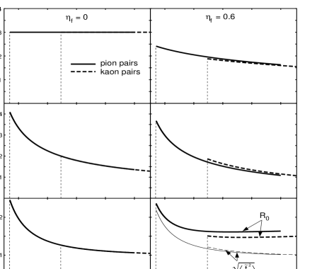
Figure 2: The YKP radii $R_{\perp}$, $R_{\parallel}$, and $R_{0}$ (top to bottom) for zero transverse flow (left column) and for $\eta_{f}=0.6$ (right column), as functions of $M_{\perp}$ for pairs at $Y_{\rm cm}=0$. Solid (dashed) lines are for pions (kaons). The breaking of the $M_{\perp}$-scaling by transverse flow is obvious in the right column. For nonzero transverse flow $R_{0}$ also does not agree exactly with the effective source lifetime $\sqrt{\langle\tilde{t}^{2}\rangle}$ (lower right panel). Source parameters as in Fig. 1.

The transverse radius parameter $R_{\perp}$ is invariant under longitudinal boosts and thus not affected at all by longitudinal expansion (upper left panel in Fig. 2). It begins, however, to drop as a function of $M_{\perp}$ if the source expands in the transverse directions (upper right panel). Comparing the lower two left and right panels in Fig. 2 one sees that the sensitivity of $R_{\parallel}$ and $R_{0}$ to transverse flow is much weaker.$\!{}^{{\bf?}}$ Transverse (longitudinal) flow thus mostly affects the transverse (longitudinal) regions of homogeneity.

While longitudinal “flow” is not necessarily a signature for nuclear collectivity but could be “faked” as discussed at the end of the previous subsection, transverse flow is much more generic in this respect: the ingoing channel has no transverse collective motion, and the only mechanism imaginable for the creation of transverse collective dynamics during the collision is multiple (re-)scattering among the secondaries, leading ultimately to hydrodynamic transverse flow.

Unfortunately, the observation of an $M_{\perp}$-dependence of $R_{\perp}$ by itself is not sufficient to prove the existence of radial transverse flow. It can also be created by other types of transverse gradients, e.g. a transverse temperature gradient.$\!{}^{{\bf?},\penalty 1000\ {\bf?},\penalty 1000\ {\bf?}}$ To exclude such a possibility one must check the $M_{\perp}$-scaling of the YKP radii, i.e. the independence of the functions $R_{i}(M_{\perp})$ ($i=\perp,\parallel,0$) of the particle rest mass (which is not broken by temperature gradients). Since different particle species are affected differently by resonance decays, such a check further requires the elimination of resonance effects.

6 Resonance decays

Resonance decays contribute additional pions at low $M_{\perp}$; these pions originate from a larger region than the direct ones, due to resonance propagation before decay. They cause an $M_{\perp}$-dependent modification of the HBT radii.

Quantitative studies $\!{}^{{\bf?},\penalty 1000\ {\bf?}}$ have shown that the resonances can be subdivided into three classes with different characteristic effects on the correlator:
(i) Short-lived resonances with lifetimes up to a few fm/$c$ do not propagate far outside the region of thermal emission and thus affect $R_{\perp}$ only marginally. They contribute to $R_{0}$ and $R_{\parallel}$ up to about 1 fm via their lifetime; $R_{\parallel}$ is larger if pion emission occurs later because for approximately boost-invariant expansion the longitudinal velocity gradient decreases as a function of time.
(ii) Long-lived resonances with lifetimes of more than several hundred fm/$c$ do not contribute to the measured correlation and thus only reduce the correlation strength (the intercept at $q=0$), without changing the shape of the correlator. Decaying at large distances from their production point, they simulate a very large source which contributes to the correlation signal only for unmeasurably small relative momenta.
(iii) Only the $\omega$ meson with its lifetime of 23.4 fm/$c$ does not fall in either of these two classes and can thus distort the form of the correlation function. It contributes a second bump at small $q$ to the correlator, giving it a non-Gaussian shape and thus complicating $\!{}^{{\bf?}}$ the extraction of HBT radii from a Gaussian fit. At small $M_{\perp}$ up to 10% of the pions can come from $\omega$ decays, and this fraction doubles effectively in the correlator since the other pion can be a direct one; thus the effect is not always negligible.

Figure 3: The inverted $q$-variance $R_{\perp}$ and the kurtosis $\Delta_{\perp}$ (the index $s$ in the figure stands for “sideward”) at $Y=0$ as functions of $K_{\perp}$. Left: $\eta_{f}=0$ (no transverse flow). Right: $\eta_{f}=0.3$. The difference between dashed and solid lines is entirely dominated by $\omega$ decays. Source parameters as in Fig. 1, except for $R=5$ fm.

In a detailed model study $\!{}^{{\bf?}}$ we showed that resonance contributions can be identified through the non-Gaussian features in the correlator induced by the tails in the emission function resulting from resonance decays. To this end one computes the second and fourth order $q$-moments of the correlator.$\!{}^{{\bf?}}$ The second order moments define the HBT radii, while the kurtosis (the normalized fourth order moments) provide a lowest order measure for the deviations from a Gaussian shape. We found $\!{}^{{\bf?}}$ that, at least for the model (33), a positive kurtosis can always be associated with resonance decay contributions (Fig. 3, left panel). Strong flow also generates a non-zero, but small and apparently always negative kurtosis (Fig. 3, right panel). Any $M_{\perp}$-dependence of $R_{\perp}$ which is associated with a positive $M_{\perp}$-dependent kurtosis must therefore be regarded with suspicion; an $M_{\perp}$-dependence of $R_{\perp}$ with a vanishing or negative kurtosis, however, cannot be blamed on resonance decays.

In our model, the first situation is realized for a source without transverse expansion (left panel of Fig. 1): At small $M_{\perp}$ the $\omega$ contribution increases $R_{\perp}$ by up to 0.5 fm while for $M_{\perp}>600$ MeV it dies out. The effect on $R_{\perp}$ is small because the heavy $\omega$ moves slowly and doesn’t travel very far before decaying. The resonance contribution is clearly visible in the positive kurtosis (lower curve). For non-zero transverse flow (right panel) there is no resonance contribution to $R_{\perp}$; this is because for finite flow the effective source size for the heavier $\omega$ is smaller than for the direct pions, and the $\omega$-decay pions thus always remain buried under the much more abundant direct ones. Correspondingly the kurtosis essentially vanishes; in fact, it is slightly negative, due to the weak non-Gaussian features induced by the transverse flow.

7 Opaque sources

The emission function (33) is only one of an infinity of possible source parametrizations. Its form permits, however, easy implementation of most of the important features of the sources created in heavy ion collisions. Still, there is one important physical situation which cannot be parametrized by the formula (33): if the source emits particles not from the entire volume, but only from a thin surface layer. This is how the sun radiates photons, and this is also an often suggested picture for the slow hadronization of long-lived QGP blobs through a deflagration-type strong first order transition.

The significance of such a phenomenon for HBT interferometry was realized by Heiselberg and Vischer $\!{}^{{\bf?}}$ who pointed out that an effective emission region which is part of a thin surface layer has a much smaller extension in the “outward” or $x$-direction than in the “sideward” or $y$-direction. In other words, such “opaque sources” have $\langle\tilde{x}^{2}-\tilde{y}^{2}\rangle<0$. Depending on the degree of opacity (the thickness of the surface layer relative to the source radius) this difference can be large and negative. The authors pointed out $\!{}^{{\bf?}}$ that this leads to the possibility of a smaller “outward” than “sideward” HBT radius parameter in the Pratt-Bertsch parametrization, even at $K_{\perp}=0$. Recently B. Tomášik showed $\!{}^{{\bf?}}$ that in the YKP parametrization opacity effects would show up even more spectacularly by a “lifetime parameter” $R_{0}^{2}$ which would diverge to $-\infty$ in the limit $K_{\perp}\to 0$ resp. $\beta_{\perp}\to 0$ (see Eq. (32)).

The source (33) can be made opaque $\!{}^{{\bf?},\penalty 1000\ {\bf?}}$ by multiplying it by the factor $\exp\left(-\kappa l_{\rm eff}/\lambda)\right)$ where $\lambda$ is the mean free path and $\kappa l_{\rm eff}$ is the effective travelling distance of the emitted particle through matter in the source.$\!{}^{{\bf?}}$

Fig. 4c shows the “temporal” YKP radius parameter $R_{0}^{2}$ as a function of $M_{\perp}$ for sources with different degrees of opacity. For different opacities $R/\lambda$, the transverse source parameters $R$ and $\eta_{f}$ were readjusted $\!{}^{{\bf?}}$ to give the same measured $\!{}^{{\bf?}}$ single particle slope. The crucial features of opacity are clearly visible: the negative contribution $\sim\langle\tilde{x}^{2}-\tilde{y}^{2}\rangle$ in (32) drives $R_{0}^{2}$ to negative values at small $K_{\perp}$, and this happens the sooner the shorter the mean free path $\lambda$, i.e. the thinner the surface layer is.

Fig. 4c implies that thin surfaces with $\lambda<R$ are essentially excluded. Pion freeze-out occurs not in the form of surface emission, but happens in bulk. 160 A GeV Pb+Pb collisions are thus quite similar to the Early Universe: an early stage of complete opaqueness (here lasting for about 8 fm/$c$) is followed by a rather sudden ($\Delta\tau\sim$1-2 fm/$c$) transition to complete transparency. In both cases this transition is due to the expansion and cooling of the system, causing a rapid increase of the mean free path of the particles. In the Early Universe photon decoupling is triggered by the recombination of electrons and ions into neutral atoms; in heavy ion collisions at SPS energies pion decoupling is caused mostly by the rapid cooling and dilution of the baryon density, since baryonic resonances with their strong coupling to the pion channel provide the “glue” needed for keeping the system close to local thermal equilibrium.

Figure 4: The YKP radius parameters $R_{\perp},R_{\parallel}$, and $R_{0}^{2}$ as functions of $M_{\perp}$ for pion pairs from 158 A GeV/$c$ Pb+Pb collision $\!{}^{{\bf?}}$ at slightly forward pair rapidity $Y_{{}_{\rm CM}}=1.25$. Solid, dashed and dotted curves correspond to $R/\lambda=0,1,10$, respectively. (The corresponding pairs $(\eta_{f},R)$ are (0.4,5.74 fm), (0.345,4.83 fm), and (0.215,3.35 fm), respectively.$\!{}^{{\bf?}}$) Other source parameters: $T$=120 MeV, $\tau_{0}$=8 fm/$c$, $\Delta\tau$=2 fm/$c$, $\Delta\eta$=1.3.

8 Analysis of Pb+Pb data

Fig. 4 shows a numerical fit $\!{}^{{\bf?},\penalty 1000\ {\bf?}}$ of the YKP radius parameters, using the expressions (30)-(32) with our model source (33), to data collected by the NA49 collaboration in 158 A GeV/$c$ Pb+Pb collisions.$\!{}^{{\bf?}}$ The fit includes resonance decay contributions to the single particle spectra, but not to the 2-particle correlations. Based on sample calculations the latter are, however, expected to be inside the systematic error of the data.

The width of the pion rapidity distribution is reproduced with $\Delta\eta{=}1.3$. $\tau_{0}$ and $\Delta\eta$ are then fixed $\!{}^{{\bf?}}$ by the magnitude of $R_{\parallel}$ and $R_{0}$. The magnitude of $R_{\perp}(K_{\perp}=0)$ fixes the radius $R$ once $T$ and $\eta_{f}$ are known. The latter are obtained from the $M_{\perp}$-dependence of $R_{\perp}$, albeit not independently: essentially only the combination $\eta_{f}\sqrt{M_{\perp}/T}$ (the velocity gradient divided by the thermal smearing factor) can be extracted.$\!{}^{{\bf?},\penalty 1000\ {\bf?}}$ This is similar to the single particle spectra whose $M_{\perp}$-slopes determine only an effective blushifted temperature,$\!{}^{{\bf?}}$ $T_{\rm eff}=T\sqrt{{1+\bar{v}_{f}\over 1-\bar{v}_{f}}}$. The correlations between $T$ and $\eta_{f}$ are, however, exactly opposite in the two cases: for a fixed spectral slope $T$ must be decreased if $\eta_{f}$ increases while a fixed $M_{\perp}$-slope of $R_{\perp}$ requires decreasing values of $\eta_{f}$ if $T$ is reduced.$\!{}^{{\bf?}}$ The combination of single-particle spectra and two-particle correlation thus allows for a separate determination of $T$ and $\eta_{f}$.

The fit in Fig. 4 corresponds to an average transverse flow velocity $\bar{v}_{f}{=}0.44$, combined with a freeze-out temperature of about 120 MeV. Similar values were advocated by Kämpfer $\!{}^{{\bf?}}$ based on a simultaneous analysis of single particle spectra of various different hadron species from Pb+Pb collisions.

Let us discuss in more detail the numbers resulting from this fit. First, the transverse size parameter $R\approx 6$ fm is surprisingly large. At mid-rapidity even larger values ($R\simeq 7$ fm) are required.$\!{}^{{\bf?},\penalty 1000\ {\bf?}}$ Resonance contributions are not expected to reduce it by more than 0.5 fm.$\!{}^{{\bf?}}$ The transverse flow correction to $R_{\perp}$ is appreciable, resulting in a visible transverse homogeneity length of only about 5 fm at small $K_{\perp}$, but even this number is large. $R{=}6$-7 fm corresponds to an r.m.s. radius $r_{\rm rms}=\sqrt{\langle\tilde{x}^{2}+\tilde{y}^{2}\rangle}\approx 8.5$-10 fm of the pion source, to be compared with an r.m.s. radius $r_{\rm rms}^{\rm Pb}=1.2\times A^{1/3}*\sqrt{2/5}$ fm = 4.5 fm for the density distribution of the original Pb nucleus projected on the transverse plane. This implies a transverse expansion of the reaction zone by a linear factor $\simeq 2$. That we also find a large transverse flow velocity renders the picture consistent. The longitudinal size of the collision region at the point where the pressure in the system began to drive the transverse expansion can be estimated as follows: for the source to expand in, say, the $y$-direction from $\sqrt{\langle y^{2}\rangle}_{\rm initial}=1.2\,A^{1/3}/\sqrt{5}$ fm = 3.2 fm to $\sqrt{\langle y^{2}\rangle}_{\rm final}=R\approx 6$ fm with an average transverse flow velocity of at most $\bar{v}=0.44\,c$ (the freeze-out value determined from the fit shown in Fig. 4) requires a time of at least $(6-3.2)/0.44$ fm/$c\simeq 6.5$ fm/$c$. Due to the selfsimilarity of the longitudinal expansion the longitudinal dimension of the source grows linearly with $\tau$. If the total expansion time until freeze-out is given by the fit parameter $\tau_{0}=8$ fm/$c$, the source expanded in the $\simeq 6.5$ fm/$c$ during which there was transverse expansion by a factor 8/(8-6.5) = 8/1.5 $\simeq 5$ in the longitudinal direction. We conclude that the fireball volume must have expanded by a factor $5*2^{2}\approx 20$ between the onset of transverse expansion and freeze-out! This is the clearest evidence for strong collective dynamical behaviour in ultra-relativistic heavy-ion collisions so far.

The local comoving energy density at freeze-out can be estimated from the fitted values for $T$ and $\eta_{f}$. The thermal energy density of a hadron resonance gas at $T=120$ MeV and moderate baryon chemical potential is of the order of 100 MeV/fm³. The large average transverse flow velocity of $\langle v_{f}\rangle\approx 0.44$ implies that about 25% flow energy must be added in the lab frame. This results in an estimate of about $0.1$ GeV/fm${}^{3}\times 1.25\times 20\approx$ 2.5 GeV/fm³ for the energy density of the reaction zone at the onset of transverse expansion. This is well above the critical energy density $\epsilon_{\rm cr}\leq 0.9$ GeV/fm³ predicted by lattice QCD for deconfined quark-gluon matter.$\!{}^{{\bf?}}$ Whether this energy density was fully thermalized is, of course, a different question. It must, however, have been accompanied by transverse pressure (i.e. some degree of equilibration of momenta must have occurred already before this point), because otherwise transverse expansion could not have been initiated.

9 Conclusions

I hope to have shown that

• two-particle correlation functions from heavy-ion collisions provide valuable information both on the geometry and the dynamical state of the reaction zone at freeze-out;

• a comprehensive and simultaneous analysis of single-particle spectra and two-particle correlations, with the help of models which provide a realistic parametrization of the emission function, allows for an essentially complete reconstruction of the final state of the reaction zone, which can serve as a reliable basis for theoretical back-extrapolations towards the interesting hot and dense early stages of the collision;

• simple and conservative estimates, based on the crucial new information from HBT measurements on the large transverse size of the source at freeze-out and using only energy conservation, lead to the conclusion that in Pb+Pb collisions at CERN, before the onset of transverse expansion, the energy density exceeded comfortably the critical value for the formation of a color deconfined state of quarks and gluons. There is, however, no evidence for long time delays due to hadronization of the QGP, and pions freeze out in bulk rather than from the surface of the collision fireball. This is in line with lattice results which predict at most a weakly first order confinement transition, and with other evidence $\!{}^{{\bf?}}$ for rapid hadronization.

I would like to thank the organizers of CRIS98 for their hospitality and support. The results reported here were obtained in collaboration with D. Anchishkin, S. Chapman, P. Scotto, C. Slotta, B. Tomášik, U. Wiedemann, Y.-F. Wu, and Q.H. Zhang. Our work was supported by grants from DAAD, DFG, NSFC, BMBF, GSI and the Alexander von Humboldt Foundation.

References

References

• [1] R. Hanbury Brown and R.Q. Twiss, Phil. Mag. 45, 633 (1954); and Nature 177, 27 (1956); 178, 1046 and 1447 (1956).
• [2] G. Goldhaber, S. Goldhaber, W. Lee, and A. Pais, Phys. Rev. 120, 300 (1960).
• [3] J. Schmidt-Sörensen, this volume, and references therein.
• [4] U. Heinz and Q.H. Zhang, Phys. Rev. C 56, 426 (1997); H. Heiselberg and A. Vischer, nucl-th/9707036.
• [5] K.S. Lee and U. Heinz, Z. Phys. C 43, 425 (1989); K.S. Lee, U. Heinz and E. Schnedermann, Z. Phys. C 48, 525 (1990); E. Schnedermann and U. Heinz, Phys. Rev. Lett. 69, 2908 (1992); E. Schnedermann, J. Sollfrank and U. Heinz, Phys. Rev. C 48, 2462 (1993); E. Schnedermann and U. Heinz, Phys. Rev. C 50, 1675 (1994); U. Heinz, in Hot Hadronic Matter: Theory and Experiment, (J. Letessier et al., eds.), NATO ASI Series B346 (Plenum, New York, 1995), p. 413.
• [6] J. Stachel et al., [E814 Collaboration], Nucl. Phys. A 566, 183c (1994); P. Braun-Munzinger et al., Phys. Lett. B 344, 43 (1995).
• [7] See proceedings of Quark Matter 96, Nucl. Phys. A 610 (1996), and of Quark Matter 97, Nucl. Phys. A (1998), in press.
• [8] M. Herrmann and G.F. Bertsch, Phys. Rev. C 51, 328 (1995).
• [9] S. Chapman, P. Scotto and U. Heinz, Phys. Rev. Lett. 74, 4400 (1995); and Heavy Ion Physics 1, 1 (1995).
• [10] S. Chapman, J.R. Nix and U. Heinz, Phys. Rev. C 52, 2694 (1995).
• [11] S. Pratt, Phys. Rev. Lett. 53, 1219 (1984); Phys. Rev. D 33, 1314 (1986).
• [12] A.N. Makhlin and Yu.M. Sinyukov, Z. Phys. C 39, 69 (1988).
• [13] S.V. Akkelin and Y.M. Sinyukov, Phys. Lett. B 356, 525 (1995).
• [14] T. Csörgő and B. Lörstad, Phys. Rev. C 54, 1396 (1996).
• [15] B. Tomášik and U. Heinz, Eur. Phys. J. C (23. Feb. 1998) (online publication) [nucl-th/9707001].
• [16] U.A. Wiedemann, P. Scotto and U. Heinz, Phys. Rev. C 53, 918 (1996).
• [17] U. Heinz et al., Phys. Lett. B 382, 181 (1996); Wu Y.-F. et al., Eur. Phys. J. C 1, 599 (1998).
• [18] B.R. Schlei et al., Phys. Lett. B 293, 275 (1992); J. Bolz et al., ibid. 300, 404 (1993); Phys. Rev. D 47, 3860 (1993).
• [19] U.A. Wiedemann and U. Heinz, Phys. Rev. C 56, R610 (1997); and Phys. Rev. C 56, 3265 (1997).
• [20] U. Heinz, in Correlations and Clustering Phenomena in Subatomic Physics, (M.N. Harakeh et al., eds.), NATO ASI Series B359 (Plenum, New York, 1997), p. 137.
• [21] M. Gyulassy, S.K. Kauffmann, and L.W. Wilson, Phys. Rev. C 20, 2267 (1979).
• [22] E. Shuryak, Phys. Lett. B 44, 387 (1973); Sov. J. Nucl. Phys. 18, 667 (1974).
• [23] S. Chapman and U. Heinz, Phys. Lett. B 340, 250 (1994).
• [24] D. Anchishkin, U. Heinz, and P. Renk, Phys. Rev. C 57, 1428 (1998).
• [25] Q.H. Zhang, U.A. Wiedemann, C. Slotta, and U. Heinz, Phys. Lett. B 407, 33 (1997).
• [26] U.A. Wiedemann et al., Phys. Rev. C 56, R614 (1997).
• [27] T. Csörgő and J. Zimányi, Phys. Rev. Lett. 80, 916 (1998); J. Zimányi and T. Csörgő, hep-ph/9705432.
• [28] U.A. Wiedemann, nucl-th/9801009
• [29] D. Pelte and H. Merlitz, this volume, and references therein [nucl-th/9806049].
• [30] H.W. Barz, Phys. Rev. C 53, 2536 (1996); S. Pratt and M.B. Tsang, Phys. Rev. C 36, 2390 (1987).
• [31] D. Anchishkin and U. Heinz, in preparation.
• [32] U. Heinz and U.A. Wiedemann, in preparation.
• [33] D.A. Brown and P. Danielewicz, Phys. Lett. B 398, 252 (1997); and Phys. Rev. C 57, 2474 (1998).
• [34] U. Heinz, in: Proceedings of the 5th International Workshop on Relativistic Aspects of Nuclear Physics, (T. Kodama et al., eds.), World Scientific, Singapore, 1998, in press [nucl-th/9710065].
• [35] J. Ellis, K. Geiger, U. Heinz and U.A. Wiedemann, in preparation.
• [36] I.V. Andreev, M. Plümer, and R.M. Weiner, Int. J. Mod. Phys. A 8, 4577 (1993).
• [37] H. Heiselberg and A.P. Vischer, Eur. Phys. J. C 2, 593 (1998).
• [38] B. Tomášik and U. Heinz, nucl-th/9805016, subm. to Eur. Phys. J. C .
• [39] H. Appelshäuser et al. (NA49 Collaboration), Eur. Phys. J. C 2, 661 (1998); P.G. Jones et al. (NA49 Collaboration), Nucl. Phys. A 610, 188c (1996); R. Ganz, this volume.
• [40] T. Alber et al. (NA35 Collaboration), Z. Phys. C 66, 77 (1995).
• [41] U.A. Wiedemann, B. Tomášik, and U. Heinz, in Quark Matter 97, Nucl. Phys. A (1998), in press [nucl-th/9801017].
• [42] S. Schönfelder, PhD thesis, MPI für Physik, München (1996).
• [43] B. Kämpfer, nucl-th/9612336, and private communication.
• [44] E. Laermann, Nucl. Phys. A 610, 1c (1996).
• [45] J. Letessier, A. Tounsi, U. Heinz, J. Sollfrank, and J. Rafelski, Phys. Rev. C 51, 3408 (1995).