Taming the Penguin in the $B^{0}_{d}(t)\rightarrow\pi^{+}\pi^{-}$ CP-Asymmetry: Observables and Minimal Theoretical Input

Abstract

Penguin contributions, being not negligible in general, can hide the information on the CKM angle $\alpha$ coming from the measurement of the time-dependent $B^{0}_{d}(t)\rightarrow\pi^{+}\pi^{-}$ CP-asymmetry. Nevertheless, we show that this information can be summarized in a set of simple equations, expressing $\alpha$ as a multi-valued function of a single theoretically unknown parameter, which conveniently can be chosen as a well-defined ratio of penguin to tree amplitudes. Using these exact analytic expressions, free of any assumption besides the Standard Model, and some reasonable hypotheses to constrain the modulus of the penguin amplitude, we derive several new upper bounds on the penguin-induced shift $|2\alpha-2\alpha_{\rm eff}|$, generalizing the recent result of Grossman and Quinn. These bounds depend on the average branching ratios of some decays ($\pi^{0}\pi^{0}$, $K^{0}\overline{K^{0}}$, $K^{\pm}\pi^{\mp}$) particularly sensitive to the penguin. On the other hand, with further and less conservative approximations, we show that the knowledge of the $B^{\pm}\rightarrow K\pi^{\pm}$ branching ratio alone gives sufficient information to extract the free parameter without the need of other measurements, and without knowing $|V_{td}|$ or $|V_{ub}|$. More generally, knowing the modulus of the penguin amplitude with an accuracy of $\sim 30\%$ might result in an extraction of $\alpha$ competitive with the experimentally more difficult isospin analysis. We also show that our framework allows to recover most of the previous approaches in a transparent and simple way, and in some cases to improve them. In addition we discuss in detail the problem of the various kinds of discrete ambiguities.

LPTHE-Orsay 98-35

hep-ph/9806468

1 Introduction

In a close future, several collaborations—BaBar, BELLE, CDF, CLEO, HERA-B—will hopefully make the first measurements of CP-violation in the $B_{d}$ system [1]. The most important consequences concerning the Standard Model (SM) would be the determination of the Unitarity Triangle (UT). However, if the measurement of the UT angle $\sin 2\beta$ seems to be straightforward from both experimental and theoretical points of view thanks to the very clean $B\rightarrow J/\Psi K_{S}$ decay, the extraction of $\alpha$ from the standard mode $B\rightarrow\pi^{+}\pi^{-}$ is still an open problem . Since it has been pointed out that QCD—and mixed QCD/electroweak—radiative corrections (called “penguins”) induce potentially large theoretical uncertainties on this angle [2], many papers have been devoted to this subject [3].

In a pioneering paper [4], Gronau and London have shown that the knowledge of the $B(\overline{B})\rightarrow\pi^{+}\pi^{-},\pi^{0}\pi^{0},\pi^{\pm}\pi^{0}$ branching ratios leads to the determination of the gluonic penguin effects, assuming isospin symmetry and neglecting electroweak penguin contributions. Then, with this information and the usual mixing-induced CP-asymmetry it is possible to get $\alpha$ up to discrete ambiguities. The main drawback of this interesting method is the expected smallness of the $B\rightarrow\pi^{0}\pi^{0}$ branching ratio ($10^{-7}$–$10^{-6}$) due to colour-suppression. This fact, combined with the detection efficiency of the final state and the needed tagging of the flavour of the $B$-meson, constitutes a difficult challenge to $e^{+}e^{-}$ $B$-factories and an almost impossible task for future hadronic machines—LHCb, BTeV.

Then it was realized by Silva and Wolfenstein [5] that by extending the flavour symmetry to SU(3) one can gain further information on penguin effects, the key point being the $K\pi$ modes where the ratio penguin/tree is certainly greater than 1. Considering the crudeness of the assumptions made in the original paper in addition to SU(3), the method has been extended until a high level of sophistication by several authors [6]. As a consequence, it is not clear to what extent such complicated geometrical constructions, plagued by multiple discrete ambiguities, are sensitive to $\alpha$ and to the unavoidable theoretical assumptions. Therefore these strategies will give conservative results only when a better understanding of non-leptonic $B$-decays is available. In addition, two simpler SU(3) approaches concerning $\alpha$ have been proposed by Buras and Fleischer [7] and Fleischer and Mannel [8] respectively, which will be discussed in more detail below.

One can also use a model—usually factorization—to estimate the penguin amplitude, and then compute the difference between $\alpha$ at the input and $\alpha_{\rm eff}$ at the output, as Aleksan et al. [9] and Ciuchini et al. [10] did, or directly get a model-dependent $\alpha$ as was proposed by Marrocchesi and Paver [11] .

Thus, after having hunted [12], trapped [13] and made the zoology [8] of the penguin, it is time to begin taming it. To accomplish this task, we first remark that most of the authors cited above have computed the observables—branching ratio and CP-asymmetries—as functions of the theoretical parameters—QCD matrix elements and CKM factors, including the angle $\alpha$. We will follow the opposite way, and show that it is indeed a fruitful approach. Although fully equivalent to the “traditional” one, it leads to a very important and simple new result: it is possible to express independently of any model , and in an exact and simple way all the theoretical parameters, including the angle $\alpha$, as functions of the experimentally accessible observables and of only one real theoretical unknown. The latter can be chosen as, e.g., $|P/T|$, the ratio of “penguin” to “tree” amplitudes (which are unambiguously defined below). It is also possible to use as the unknown a pure QCD quantity, free of any dependence with respect to $|V_{td}|$ or $|V_{ub}^{\ast}|$ contrary to the parameter $|P/T|$; in the latter case, we give polynomial equations directly expressed in the $(\rho,\eta)$ plane. We have exploited these exact analytic expressions to derive several new and simple results and to recover some of the previous approaches. The main points of this paper are:

• Using the exact parametrization in terms of $|P/T|$, it is possible to represent the information given by the time-dependent CP-asymmetry in the $(|P/T|,2\alpha)$ plane. Of course without any further assumption on the magnitude of $|P/T|$ there is no way to constrain $\alpha$. But this $(|P/T|,2\alpha)$ plot provides a nice transparent presentation of experimental data, where our ignorance of the strong interactions is relegated to a single parameter.

• As soon as one is interested in quantifying the size of the penguin—and indeed we are, $\sin 2\alpha$ is not a good parameter. One should simply use $2\alpha$ instead. Actually using $\sin 2\alpha$ rather than $2\alpha$ is not wrong, but one loses half of the information as we will see in detail below. This is already true at the level of the parametrization in terms of $|P/T|$, and this is also true for all the methods allowing to remove the penguin effects, which give generically $2\alpha$ rather than $\sin 2\alpha$, up to discrete ambiguities. To make clear this point which up to now has remained confused, we will treat explicitly the example of the Gronau-London isospin analysis. On the contrary, the observables depend only on $2\alpha$ or equivalently on $\tan\alpha$, and thus the $\alpha\rightarrow\pi+\alpha$ ambiguity is always present [14].

• Bounding the magnitude of the penguin allows directly to bound the shift of the CKM angle $\alpha$ from the directly observable $\alpha_{\rm eff}$. This can be done using information from decays particularly sensitive to the penguin. For example, assuming SU(2) isospin symmetry and neglecting electroweak penguin contributions we are able to derive two bounds depending on $\mbox{{\rm BR}}(B\rightarrow\pi^{0}\pi^{0})$, one of which being the Grossman-Quinn bound [15] while the other is new. Assuming the larger SU(3) symmetry, we obtain two new bounds depending on $\mbox{{\rm BR}}(B\rightarrow K^{0}\overline{K^{0}})$ and $\lambda^{2}\mbox{{\rm BR}}(B\rightarrow K^{\pm}\pi^{\mp})$ respectively which, not surprisingly, may be more constraining than the SU(2) ones, and which need some, but not all, the usual assumptions concerning the neglect of annihilation and/or electroweak penguin diagrams. As far as the branching ratios of the penguin-sensitive modes are concerned, these bounds do not need flavour tagging and are still valid when only an upper limit on the branching ratios is available. In addition, they can be slightly modified to be used when the actual value of the direct CP-asymmetry in the $B\rightarrow\pi^{+}\pi^{-}$ channel is not available, as it is shown below. Depending on the actual values of the branching ratios, the theoretical error on $\alpha$ constrained by these bounds could be as large as $\sim 30^{\circ}$ or as small as $\sim 10^{\circ}$. In particular, the most recent CLEO analyses of the $\pi^{+}\pi^{-}$ and $K^{\pm}\pi^{\mp}$ modes [16] allow us to give for the first time the following numerical bound

  $$|2\alpha-2\alpha_{\rm eff}|\leq\Delta\,,\ \ \ \mbox{with}\ \ \ 25^{\circ}<\Delta<59^{\circ}$$ (1)

  assuming rather weak hypotheses in the SU(3) limit (see § 5.2) and BR$(B\rightarrow\pi^{+}\pi^{-})>0.4\times 10^{-5}$ in addition to the CLEO data.

• Finally, after having stressed that only one hadronic parameter has to be estimated by the theory in order to get $\alpha$, we give one new explicit example: assuming SU(3) and neglecting annihilation and electroweak penguin diagrams, we show that $\mbox{{\rm BR}}(B^{\pm}\rightarrow K\pi^{\pm})$ gives sufficient information to solve a degree-four polynomial equation in the $(\rho,\eta)$ plane, which roots can be represented as curves in this plane. Contrary to the Fleischer-Mannel proposal [8], ours does not need the knowledge of $|V_{td}|$ or $|V_{ub}|$, and requires only the measurement of $\mbox{{\rm BR}}(B^{\pm}\rightarrow K\pi^{\pm})$ in addition to the usual time-dependent $B\rightarrow\pi^{+}\pi$ time-dependent CP-asymmetry. Alternatively, the knowledge of the modulus of the penguin amplitude (or the ratio of penguin to tree) with an uncertainty of $\sim 30\%$ should provide a rather good estimation of $\alpha$. This kind of strategy, although affected by potentially large theoretical uncertainties, may be necessary when the more conservative bounds are too weak to be really useful in testing the SM.

The paper is organized as follows: in Section 2, we summarize the main results of this work—this section should be of immediate use for the reader not interested by the development. In Section 3 we fix our notations in writing the general parametrization of the amplitudes. With the help of the recent CLEO measurements of non-leptonic charmless $B$-decays, we give some rough orders of magnitude of the expected penguin pollution. Then we derive the equations giving the theoretical parameters, including $\alpha$, as functions of the observables and the theoretical unknown, treated first as a free parameter, and latter eventually constrained under reasonable hypotheses. For example in Section 4 we show how to use in our framework the information coming from the $B\rightarrow\pi^{0}\pi^{0}$ and $B^{\pm}\rightarrow\pi^{\pm}\pi^{0}$ decays, to obtain the Grossman-Quinn bound and a new similar isospin bound. In Section 5 we exhibit two new bounds, based on the SU(3) assumption, which may be more stringent than the two isospin bounds. Then in Section 6 we discuss an explicit example where the theoretical unknown is actually estimated rather than bounded. A reasonable knowledge of $\alpha$ can be expected even if one allows a sizeable violation of the theoretical assumptions. In Section 7 we discuss how to incorporate and improve some of the previous approaches in our language, and clarify some points which have been mistreated in the literature, in particular the problem of the discrete ambiguities. Our conclusion is that although the penguin-induced error on $\alpha$ is expected to be quite large in the $B\rightarrow\pi^{+}\pi^{-}$ channel, it should be under the control of the theory. Therefore the generalization of the methods presented here to other channels is very desirable to get more constraints on $\alpha$.

This paper has two technical appendices: the first one (A) explains how we got the values of the observables from a naive calculation, in order to numerically illustrate our purpose before experimental data is available and the second one (B), following Grossman and Quinn [15], shows explicitly the existence of bounds which are independent of the measurement of the direct CP-asymmetry.

2 Summary

2.1 Exact Model-Independent Results

Defining the Standard Model $B\rightarrow\pi^{+}\pi^{-}$ amplitudes

$$A(B^{0}\rightarrow\pi^{+}\pi^{-}) = V_{ud}V_{ub}^{\ast}M^{(u)}+V_{td}V_{tb}^{\ast}M^{(t)}\ =\ e^{+i\gamma}T+e^{-i\beta}P\,,$$ (2)

$$A(\overline{B^{0}}\rightarrow\pi^{+}\pi^{-}) = V_{ud}^{\ast}V_{ub}M^{(u)}+V_{td}^{\ast}V_{tb}M^{(t)}\ =\ e^{-i\gamma}T+e^{+i\beta}P\,,$$ (3)

the time-dependent $B^{0}(t)\rightarrow\pi^{+}\pi^{-}$ CP-asymmetry

$$a_{\rm CP}(t)=a_{\rm dir}\cos\Delta m\,t-\sqrt{1-a_{\rm dir}^{2}}\sin 2\alpha_{\rm eff}\sin\Delta m\,t\,,$$ (4)

and the average $B,\overline{B}\rightarrow f,\bar{f}$ branching ratio

$${\cal B}_{f,\bar{f}}=\frac{1}{2}\left[\mbox{{\rm BR}}(B\rightarrow f)+\mbox{{\rm BR}}(\overline{B}\rightarrow\bar{f})\right]\,,$$ (5)

we prove in the following that the Standard Model predicts very simple relations between $\alpha$ and $|P/T|$, $|P|$, $|T|$ and $\delta={\rm Arg}(PT^{\ast})$ respectively, these relations depending only on the observables ${\cal B}_{\pi^{+}\pi^{-}}$, $a_{\rm dir}$ and $2\alpha_{\rm eff}$ and being completely free of any assumption on hadronic physics:

$$\cos(2\alpha-2\alpha_{\rm eff}) = \frac{1}{\sqrt{1-a_{\rm dir}^{2}}}\left[1-\left(1-\sqrt{1-a_{\rm dir}^{2}}\cos 2\alpha_{\rm eff}\right)\left|\frac{P}{T}\right|^{2}\,\right]\,,$$ (6)

$$|P|^{2} = \frac{{\cal B}_{\pi^{+}\pi^{-}}}{1-\cos 2\alpha}\left[1-\sqrt{1-a_{\rm dir}^{2}}\cos(2\alpha-2\alpha_{\rm eff})\right]\,,$$ (7)

$$|T|^{2} = \frac{{\cal B}_{\pi^{+}\pi^{-}}}{1-\cos 2\alpha}\left[1-\sqrt{1-a_{\rm dir}^{2}}\cos 2\alpha_{\rm eff}\right]\,,$$ (8)

$$\tan\delta = \frac{a_{\rm dir}\tan\alpha}{1-\sqrt{1-a_{\rm dir}^{2}}\left[\cos 2\alpha_{\rm eff}+\tan\alpha\sin 2\alpha_{\rm eff}\right]}\,.$$ (9)

Rather than $|P/T|$, $|P|$ and $|T|$ which incorporate respectively a $|V_{td}/V_{ub}^{\ast}|$, $|V_{td}|$ and $|V_{ub}^{\ast}|$ factor, one may prefer to write Eqs. (6-8) in terms of $|M^{(t)}/M^{(u)}|$, $|M^{(t)}|$ and $|M^{(u)}|$ respectively (see the definition (2)). As $|V_{td}|$ and $|V_{ub}^{\ast}|$ depend also on the UT, it is not possible to express such relations as functions of $\alpha$ alone; instead we use the Wolfenstein parametrization and find three polynomial equations in the $(\rho,\eta)$ plane. With the definitions of the following combinations of observables

$$D_{c}\equiv\sqrt{1-a_{\rm dir}^{2}}\cos 2\alpha_{\rm eff}\,,\ \ \ \ \ D_{s}\equiv\sqrt{1-a_{\rm dir}^{2}}\sin 2\alpha_{\rm eff}\,,$$ (10)

and the theoretical parameters $|M^{(t)}|$ and $|M^{(u)}|$ normalized to $\sqrt{{\cal B}_{\pi^{+}\pi^{-}}}/|\lambda V_{cb}|$

$$\frac{R_{P}}{R_{T}}=\left|\frac{M^{(t)}}{M^{(u)}}\right|^{2}\,,\ \ \ \ \ R_{P}\equiv|\lambda V_{cb}|^{2}\frac{|M^{(t)}|^{2}}{{\cal B}_{\pi^{+}\pi^{-}}}\,,\ \ \ \ \ R_{T}\equiv|\lambda V_{cb}|^{2}\frac{|M^{(u)}|^{2}}{{\cal B}_{\pi^{+}\pi^{-}}}\,,$$ (11)

one has two degree-four polynoms depending respectively on $R_{P}/R_{T}$ and $R_{P}$

$$(1-D_{c})(1-\frac{R_{P}}{R_{T}})\,\rho^{4}+2(1-D_{c})(1-\frac{R_{P}}{R_{T}})\,\rho^{2}\eta^{2}+(1-D_{c})(1-\frac{R_{P}}{R_{T}})\,\eta^{4}$$

$$-2(1-D_{c})(1-2\frac{R_{P}}{R_{T}})\,\rho^{3}-2D_{s}\,\rho^{2}\eta-2(1-D_{c})(1-2\frac{R_{P}}{R_{T}})\,\rho\eta^{2}-2D_{s}\,\eta^{3}$$

$$+(1-D_{c})(1-6\frac{R_{P}}{R_{T}})\,\rho^{2}+2D_{s}\,\rho\eta+[1+D_{c}-2(1-D_{c})\frac{R_{P}}{R_{T}}]\,\eta^{2}$$

$$+(1-D_{c})\frac{R_{P}}{R_{T}}\,(4\rho-1)=0\,,$$ (12)

$$(1-D_{c})\,\rho^{4}+2(1-D_{c}-R_{P})\,\rho^{2}\eta^{2}+(1-D_{c}-2R_{P})\,\eta^{4}$$

$$-2(1-D_{c})\,\rho^{3}-2D_{s}\,\rho^{2}\eta-2(1-D_{c}-2R_{P})\,\rho\eta^{2}-2D_{s}\,\eta^{3}$$

$$+(1-D_{c})\,\rho^{2}+2D_{s}\,\rho\eta+(1+D_{c}-2R_{P})\,\eta^{2}=0\,,$$ (13)

and one linear equation depending on $R_{T}$ (the $\pm$ sign being related to a discrete ambiguity)

$$\sqrt{1-D_{c}}\,(\rho-1)\pm\sqrt{2R_{T}-1+D_{c}}\,\,\eta=0\,.$$ (14)

Eqs. (12-14) are another way of writing Eqs. (6-8) by replacing respectively $|P/T|$, $|P|$ and $|T|$ by the ratios $R_{P}/R_{T}$, $R_{P}$ and $R_{T}$: the advantage is that the latter parameters do not depend on the badly known CKM matrix elements $|V_{td}|$ and $|V_{ub}^{\ast}|$.

2.2 Phenomenological Applications

It has become standard in the CP-literature to use several phenomenological assumptions, some of which can be very good while some others can be strongly violated. As a result, it is often not easy for the reader to know exactly which approximations are used by the authors, and thus to make his own opinion about the accuracy of these theoretical prejudices. In this paper, we will try to state clearly what kind of hypotheses we use in addition to the SM; some of the results that we derive rely on a few reasonable assumptions chosen in the list below.

• Assumption 1 $|P/T|<1$. This very conservative bound should be distinguished from the small penguin expansion.

• Assumption 2 SU(2) isospin symmetry of the strong interactions.

• Assumption 3 SU(3) flavour symmetry of the strong interactions.

• Assumption 4 Neglect of the OZI-suppressed annihilation penguin diagrams (cf. Fig. 4).

• Assumption 5 Neglect of the electroweak penguin contributions.

• Assumption 6 Neglect of the $V_{us}V_{ub}^{\ast}$ contributions to the $B^{+}\rightarrow K^{0}\pi^{+}$ amplitude.

Upper Bounds.

We have found several quantities bounding the shift of the true $2\alpha$ from the experimentally accessible $2\alpha_{\rm eff}$, among which (16) is the Grossman-Quinn bound [15], while the others are new:

$$\mbox{if }\sin 2\alpha_{\rm eff}>0 0\,<\,2\alpha\,<\,2\pi-2\arcsin(\sin 2\alpha_{\rm eff})$$

$$\mbox{if }\sin 2\alpha_{\rm eff}<0 -2\arcsin(\sin 2\alpha_{\rm eff})\,<\,2\alpha\,<\,2\pi\ \ \ \ \ \mbox{[assuming~{}{\bf 1}],}$$ (15)

$$|2\alpha-2\alpha_{\rm eff}|\leq\arccos\left[\frac{1}{\sqrt{1-a_{\rm dir}^{2}}}\left(1-2\frac{{\cal B}_{\pi^{0}\pi^{0}}}{{\cal B}_{\pi^{\pm}\pi^{0}}}\right)\right]\ \ \ \ \ \mbox{[assuming~{}{\bf 2} and~{}{\bf 5}],}$$ (16)

$$|2\alpha-2\alpha_{\rm eff}|\leq\arccos\left[\frac{1}{\sqrt{1-a_{\rm dir}^{2}}}\left(1-4\frac{{\cal B}_{\pi^{0}\pi^{0}}}{{\cal B}_{\pi^{+}\pi^{-}}}\right)\right]\ \ \ \ \ \mbox{[assuming~{}{\bf 2} and~{}{\bf 5}],}$$ (17)

$$|2\alpha-2\alpha_{\rm eff}|\leq\arccos\left[\frac{1}{\sqrt{1-a_{\rm dir}^{2}}}\left(1-2\frac{{\cal B}_{K^{0}\overline{K^{0}}}}{{\cal B}_{\pi^{+}\pi^{-}}}\right)\right]\ \ \ \ \ \mbox{[assuming~{}{\bf 3} and~{}{\bf 5}],}$$ (18)

$$|2\alpha-2\alpha_{\rm eff}|\leq\arccos\left[\frac{1}{\sqrt{1-a_{\rm dir}^{2}}}\left(1-2\lambda^{2}\,\frac{{\cal B}_{K^{\pm}\pi^{\mp}}}{{\cal B}_{\pi^{+}\pi^{-}}}\right)\right]\ \ \ \ \ \mbox{[assuming~{}{\bf 3} and~{}{\bf 4}].}$$ (19)

Following Grossman and Quinn [15] we show that, under the same hypotheses, the above upper bounds still hold if one replaces in Eqs. (2.2-19) $a_{\rm dir}$ by zero and $2\alpha_{\rm eff}$ by $2\overline{\alpha}_{\rm eff}$ where the latter effective angle is defined by

$${\rm sign}(\cos 2\overline{\alpha}_{\rm eff})\equiv{\rm sign}(\cos 2\alpha)\,,\ \ \ \ \ \sin 2\overline{\alpha}_{\rm eff}\equiv\sqrt{1-a_{\rm dir}^{2}}\sin 2\alpha_{\rm eff}\,.$$ (20)

For example, one has the bound

$$|2\alpha-2\overline{\alpha}_{\rm eff}|\leq\arccos\left(1-2\lambda^{2}\,\frac{{\cal B}_{K^{\pm}\pi^{\mp}}}{{\cal B}_{\pi^{+}\pi^{-}}}\right)\ \ \ \ \ \mbox{[assuming~{}{\bf 3} and~{}{\bf 4}],}$$ (21)

and so on. Although these bounds on $|2\alpha-2\overline{\alpha}_{\rm eff}|$ are weaker than the ones on $|2\alpha-2\alpha_{\rm eff}|$, they have the advantage that they do not depend on the measurement of $a_{\rm dir}$: indeed, the angle $2\overline{\alpha}_{\rm eff}$ is accessible (up to a twofold ambiguity) from the $\sin\Delta m\,t$ term only (see Eqs. (4) and (20)). Therefore the experimental uncertainty should be smaller for $2\overline{\alpha}_{\rm eff}$ than for $2\alpha_{\rm eff}$.

In addition to these upper bounds, we derive a lower bound on $|2\alpha-2\alpha_{\rm eff}|$ in § 5.4, to which we refer the reader for more details.

Determination of $\alpha$.

We propose a new method for the extraction of $\alpha$—up to discrete ambiguities, which improves the Fleischer-Mannel proposal [8].

The idea (often used in the literature) is to estimate the modulus of the penguin contribution with the help of the $B^{\pm}\rightarrow K\pi^{\pm}$ decay. We avoid the problem of knowing $|V_{td}|$ by using directly the polynomial equation (13) in the $(\rho,\eta)$ plane, with the theoretical parameter $R_{P}$ given by

$$R_{P}=\lambda^{2}\frac{{\cal B}_{K\pi^{\pm}}}{{\cal B}_{\pi^{+}\pi^{-}}}\ \ \ \ \ \mbox{[assuming~{}{\bf 3},~{}{\bf 4},~{}{\bf 5} and~{}{\bf 6}].}$$ (22)

This typically leads to draw four allowed curves in the $(\rho,\eta)$ plane, which in the limit $R_{P}\rightarrow 0$, reduce to the two circles representing the no-penguin solution $\sin 2\alpha=\sin 2\alpha_{\rm eff}$.

3 Theoretical Framework

3.1 Standard Model Parametrization of the Amplitudes

The aim of this paragraph is to recall some already known results and to fix the notation used in this paper.

The time-dependent rate for an oscillating state $B^{0}(t)$ which has been tagged as a $B^{0}$ meson at time $t=0$ is given by (for simplicity the $e^{-\Gamma t}$ and constant phase space factors are omitted below )

$$\Gamma\left(B^{0}(t)\rightarrow\pi^{+}\pi^{-}\right)=\frac{|A|^{2}+|\bar{A}|^{2}}{2}+\frac{|A|^{2}-|\bar{A}|^{2}}{2}\cos\Delta m\,t-\mbox{{\rm Im}}\left(\frac{q}{p}\bar{A}A^{\ast}\right)\sin\Delta m\,t\,,$$ (23)

where

$$A\equiv A(B^{0}\rightarrow\pi^{+}\pi^{-})\,,\ \ \ \ \ \bar{A}\equiv A(\overline{B^{0}}\rightarrow\pi^{+}\pi^{-})$$ (24)

and $q/p=\exp(-2i\beta)$ in the Wolfenstein phase convention, which provides an expansion of the CKM matrix in powers of $\lambda\equiv|V_{us}|\sim 0.22$ [17]. With this convention, one has

$$\beta={\rm Arg}(-V_{td}^{\ast})\,,\ \ \ \ \ \gamma={\rm Arg}(-V_{ub}^{\ast})\,,\ \ \ \ \ {\rm Arg}(V_{ts})={\cal O}(\lambda^{2})\,,$$ (25)

while the other CKM matrix elements are real (up to highly-suppressed $\lambda^{n}$ terms) and the angle $\alpha$ is given by $\alpha=\pi-\beta-\gamma$. Defining

$${\cal B}_{\pi^{+}\pi^{-}} \equiv \frac{1}{2}\left[\mbox{{\rm BR}}(B^{0}\rightarrow\pi^{+}\pi^{-})+\mbox{{\rm BR}}(\overline{B^{0}}\rightarrow\pi^{+}\pi^{-})\right]\,,$$ (26)

$$a_{\rm dir} \equiv \frac{|A|^{2}-|\bar{A}|^{2}}{|A|^{2}+|\bar{A}|^{2}}\,,$$ (27)

$$2\alpha_{\rm eff} \equiv {\rm Arg}\left(\frac{q}{p}\bar{A}A^{\ast}\right)\,,$$ (28)

the rate (23) becomes

$$\Gamma\left(B^{0}(t)\rightarrow\pi^{+}\pi^{-}\right)={\cal B}_{\pi^{+}\pi^{-}}\left[1+a_{\rm dir}\cos\Delta m\,t-\sqrt{1-a_{\rm dir}^{2}}\sin 2\alpha_{\rm eff}\sin\Delta m\,t\right]\,.$$ (29)

The time-dependent CP-asymmetry reads

$$a_{\rm CP}(t) \equiv \frac{\Gamma\left(B^{0}(t)\rightarrow\pi^{+}\pi^{-}\right)-\Gamma\left(\overline{B^{0}}(t)\rightarrow\pi^{+}\pi^{-}\right)}{\Gamma\left(B^{0}(t)\rightarrow\pi^{+}\pi^{-}\right)+\Gamma\left(\overline{B^{0}}(t)\rightarrow\pi^{+}\pi^{-}\right)}$$ (30)

$$= a_{\rm dir}\cos\Delta m\,t-\sqrt{1-a_{\rm dir}^{2}}\sin 2\alpha_{\rm eff}\sin\Delta m\,t\,.$$

We may define another effective angle by 

$${\rm sign}(\cos 2\overline{\alpha}_{\rm eff})\equiv{\rm sign}(\cos 2\alpha)\,,\ \ \ \ \ \sin 2\overline{\alpha}_{\rm eff}\equiv\sqrt{1-a_{\rm dir}^{2}}\sin 2\alpha_{\rm eff}$$ (31)

such as

$$a_{\rm CP}(t)=a_{\rm dir}\cos\Delta m\,t-\sin 2\overline{\alpha}_{\rm eff}\sin\Delta m\,t\,.$$ (32)

$a_{\rm dir}$ is the direct CP-asymmetry, while $\sin 2\overline{\alpha}_{\rm eff}=\sqrt{1-a_{\rm dir}^{2}}\sin 2\alpha_{\rm eff}$ is the mixing-induced CP-asymmetry. In the absence of penguins, one has $a_{\rm dir}=0$ and $\sin 2\overline{\alpha}_{\rm eff}=\sin 2\alpha_{\rm eff}=\sin 2\alpha$. The experiment allows the measurement of three fully model-independent observables, one is CP-invariant (${\cal B}_{\pi^{+}\pi^{-}}$), while the two others are CP-asymmetries ($a_{\rm dir}$ and $\sin 2\alpha_{\rm eff}$, or $a_{\rm dir}$ and $\sin 2\overline{\alpha}_{\rm eff}$).

It has often been assumed in the literature that the dominant penguin amplitude is the top-mediated one, with the consequence that this amplitude is proportional to $V_{td}V_{tb}^{\ast}$. This assumption has received a lot of attention recently [18, 19]. In any case, the $u$-penguin contributions which are proportional to $V_{ud}V_{ub}^{\ast}$ (as well as other contributions such as exchange diagrams) can be incorporated in the definition of the “tree” amplitude. Contributions proportional to $V_{cd}V_{cb}^{\ast}$—“charming penguins” [19]—can be rewritten, by CKM unitarity ($V_{cd}V_{cb}^{\ast}=-V_{ud}V_{ub}^{\ast}-V_{td}V_{tb}^{\ast}$), in terms of the two other combinations. Thus, just from the weak phase structure of the SM, we may write the $B^{0}\rightarrow\pi^{+}\pi^{-}$ physical amplitude as

$$A = V_{ud}V_{ub}^{\ast}M^{(u)}+V_{td}V_{tb}^{\ast}M^{(t)}$$ (33)

$$\equiv e^{+i\gamma}T_{\pi^{+}\pi^{-}}+e^{-i\beta}P_{\pi^{+}\pi^{-}}$$

and similarly for the other $2\pi$ channels 

$$A_{\pi^{0}\pi^{0}}\equiv A(B^{0}\rightarrow\pi^{0}\pi^{0}) \equiv \frac{1}{\sqrt{2}}(e^{+i\gamma}\,T_{\pi^{0}\pi^{0}}+e^{-i\beta}P_{\pi^{0}\pi^{0}})\,,$$ (34)

$$A_{\pi^{+}\pi^{0}}\equiv A(B^{+}\rightarrow\pi^{+}\pi^{0}) \equiv \frac{1}{\sqrt{2}}(e^{+i\gamma}\,T_{\pi^{+}\pi^{0}}+e^{-i\beta}P_{\pi^{+}\pi^{0}})\,.$$ (35)

Let us stress that there is absolutely no approximation in writing Eq. (33-35): $T_{\pi\pi}$ and $P_{\pi\pi}$ are CP-conserving complex quantities, defined by the weak phase that they carry, and they incorporate all possible SM topologies such as trees, penguins, electroweak penguins… In this sense, many (not all, however) of the methods proposed previously for the extraction of $\alpha$ in the top-dominance assumption are in fact still valid if the latter hypothesis is relaxed . The CP-conjugate channels are obtained by reversing the sign of the weak phases:

$$\bar{A}_{\pi\pi}=e^{-i\gamma}T_{\pi\pi}+e^{+i\beta}P_{\pi\pi}\,.$$ (36)

As said above, neglecting penguin diagrams ($P_{\pi\pi}=0$) gives

$$2\alpha_{\rm eff}={\rm Arg}\left(\frac{q}{p}T_{\pi^{+}\pi^{-}}T_{\pi^{+}\pi^{-}}^{\ast}e^{-2i\gamma}\right)=2\alpha\,.$$ (37)

From now on we will denote in the whole paper

$$T_{\pi^{+}\pi^{-}}\equiv T\,,\ \ \ \ \ P_{\pi^{+}\pi^{-}}\equiv P\,,$$ (38)

and by economy of language, we will call the $T$ and $P$ amplitudes “tree” and “penguin” respectively, although $T$ gets contributions from $u$- and $c$-penguin diagrams .

In this paper, we will also consider the $B\rightarrow K^{0}\overline{K^{0}}$, $B\rightarrow K^{\pm}\pi^{\mp}$ and $B^{\pm}\rightarrow K\pi^{\pm}$ decays. For the former, we adopt the following parametrization

$$A(B^{0}\rightarrow K^{0}\overline{K^{0}}) = V_{ud}V_{ub}^{\ast}M_{K\overline{K}}^{(u)}+V_{td}V_{tb}^{\ast}M_{K\overline{K}}^{(t)}$$ (39)

$$\equiv e^{+i\gamma}\,T_{K\overline{K}}+e^{-i\beta}P_{K\overline{K}}\,,$$

while for the latter it is convenient to expand on the CKM basis $(V_{us}V_{ub}^{\ast},V_{cs}V_{cb}^{\ast})$ (recall that $V_{cs}V_{cb}^{\ast}$ is real in the Wolfenstein convention):

$$A(B^{0}\rightarrow K^{+}\pi^{-}) = V_{us}V_{ub}^{\ast}M_{K^{+}\pi^{-}}^{(u)}+V_{cs}V_{cb}^{\ast}M_{K^{+}\pi^{-}}^{(c)}$$ (40)

$$\equiv e^{+i\gamma}\,T_{K^{+}\pi^{-}}+P_{K^{+}\pi^{-}}\,,$$

$$A(B^{+}\rightarrow K^{0}\pi^{+}) \equiv e^{+i\gamma}\,T_{K^{0}\pi^{+}}+P_{K^{0}\pi^{+}}\,.$$ (41)

As far as the $B\rightarrow K^{0}\overline{K^{0}}$ amplitude is concerned, we have used the notation $T_{K\overline{K}}$ to make apparent the resemblance with the other channels; however it should be stressed that this decay is a pure penguin process. Actually $T_{K\overline{K}}$ represents the contribution of the long-distance $u$- and $c$-penguins [21].

Let us repeat that Eqs. (33-36) and (39-41) rely only on the Standard Model.

3.2 General Bounds

Similarly to Eq.( 26), we will denote by ${\cal B}_{f,\bar{f}}$ the CP-conserving average branching ratio

$${\cal B}_{f,\bar{f}}=\frac{1}{2}\left[\mbox{{\rm BR}}(B\rightarrow f)+\mbox{{\rm BR}}(\overline{B}\rightarrow\bar{f})\right]\,.$$ (42)

For example,

$${\cal B}_{K\pi^{\pm}}=\frac{1}{2}\left[\mbox{{\rm BR}}(B^{+}\rightarrow K^{0}\pi^{+})+\mbox{{\rm BR}}(B^{-}\rightarrow\overline{K^{0}}\pi^{-})\right]$$ (43)

and so on.

From the discussion in § 3.1, it is clear that the SM predicts each $B^{0}\rightarrow f$ decay amplitude as the sum of two terms carrying two different CP-violating phases $\phi_{1}$, $\phi_{2}$:

$$A(B^{0}\rightarrow f)=e^{+i\phi_{1}}M_{1}+e^{+i\phi_{2}}M_{2}\,,\ \ \ \ \ A(\overline{B^{0}}\rightarrow\bar{f})=\eta_{f}\left(e^{-i\phi_{1}}M_{1}+e^{-i\phi_{2}}M_{2}\right)$$ (44)

where $M_{1}$ and $M_{2}$, although complex numbers, are CP-conserving and the sign $\eta_{f}$ depends on the CP of the final state, e.g. $\eta_{f}(\pi^{+}\pi^{-})=+$. Thus the average branching ratio (42) writes

$${\cal B}_{f,\bar{f}}=|M_{1}|^{2}+|M_{2}|^{2}+2\,\mbox{{\rm Re}}(M_{1}M_{2}^{\ast})\cos(\phi_{1}-\phi_{2})\,.$$ (45)

Note that we express the amplitudes squared in “units of two-body branching ratio”. For fixed values of $M_{2}$ and $\phi_{1}-\phi_{2}$, ${\cal B}_{f,\bar{f}}$ as a function of $M_{1}$ takes its minimal value when $M_{1}=-M_{2}\cos(\phi_{1}-\phi_{2})$, in which case ${\cal B}_{f,\bar{f}}|_{\rm min}=|M_{2}|^{2}\sin^{2}(\phi_{1}-\phi_{2})$. Interverting the rôles of $M_{1}$ and $M_{2}$, we obtain the following (exact) general bounds:

$$|M_{1}|^{2}\sin^{2}(\phi_{1}-\phi_{2})\,\leq\,{\cal B}_{f,\bar{f}}\,,\ \ \ \ \ \ |M_{2}|^{2}\sin^{2}(\phi_{1}-\phi_{2})\,\leq\,{\cal B}_{f,\bar{f}}\,.$$ (46)

Such inequalities have been previously employed for the demonstration of the so-called Fleischer-Mannel bound [22]. We will use Eq. (46) extensively throughout this paper.

3.3 Orders of Magnitude

The recently updated CLEO analyses of $B$-decays into two light pseudoscalars give precious information on the various quantities discussed in this paper [16]:

$${\cal B}_{\pi^{+}\pi^{-}} < 0.84\times 10^{-5}\ \ [90\%\mbox{ CL}]\,,$$

$${\cal B}_{K^{\pm}\pi^{\mp}} = (1.4\pm 0.3\pm 0.2)\times 10^{-5}\,,$$ (47)

$${\cal B}_{K\pi^{\pm}} = (1.4\pm 0.5\pm 0.2)\times 10^{-5}\,.$$

Thanks to this experimental information, it is possible to derive a crude lower bound for the ratio $|P/T|$. Indeed, from Eqs. (33) and (46) we have

$$|T|^{2}\sin^{2}\alpha\,\leq\,{\cal B}_{\pi^{+}\pi^{-}}\,.$$ (48)

Furthermore, while the $\pi\pi$ penguin is proportional to $V_{td}V_{tb}^{\ast}$, the $K\pi$ penguin is proportional to $V_{cs}V_{cb}^{\ast}$ (cf. Eqs. (33) and (40-41)). Thus we have

$$|P|\sim\left|\frac{V_{td}}{V_{cb}^{\ast}}\right|\times\sqrt{{\cal B}_{s}}$$ (49)

where ${\cal B}_{s}$ is a typical scale of the $B\rightarrow K\pi$ branching ratios, assuming that these channels are dominated by the QCD penguin, and that the QCD-part of the penguin matrix elements are of the same order for $\pi\pi$ and $K\pi$. Thus we obtain

$$\left|\frac{P}{T}\right|\,{~{}\raise 1.49994pt\hbox{$>$}\kern-8.50006pt\lower 3.50006pt\hbox{$\sim$}~{}}\,\lambda|\sin\gamma|\sqrt{\frac{{\cal B}_{s}}{\,{\cal B}_{\pi^{+}\pi^{-}}}}$$ (50)

where we have used $|V_{td}/V_{cb}|=\lambda\sin\gamma/\sin\alpha$.

Numerically, from the current SM constraints on the $(\rho,\eta)$ parameters [23], we have $|\sin\gamma|{~{}\raise 1.49994pt\hbox{$>$}\kern-8.50006pt\lower 3.50006pt\hbox{$\sim$}~{}}0.6$. The CLEO data (47) suggest ${\cal B}_{s}/{\cal B}_{\pi^{+}\pi^{-}}{~{}\raise 1.49994pt\hbox{$>$}\kern-8.50006pt\lower 3.50006pt\hbox{$\sim$}~{}}1/0.84$ which gives

$$\left|\frac{P}{T}\right|\,{~{}\raise 1.49994pt\hbox{$>$}\kern-8.50006pt\lower 3.50006pt\hbox{$\sim$}~{}}\,0.14\,.$$ (51)

Note that contrary to some claims, factorization gives typically $|P/T|\sim 0.15$ [9] and is not ruled out by the CLEO data yet, although it is only marginally compatible.

Although this calculation is only illustrative, it is clear that the penguin contributions pose a serious problem for the extraction of $\alpha$ from the CP-asymmetry. More complete analyses show that the ratio $|P/T|$ can easily be $\sim$ 30% or even 40% [19]. Therefore one can not avoid to define theoretical procedures allowing to reduce the penguin uncertainty, or at least to control it. This is the subject of the present paper.

Let us add here one comment on the size of the direct CP-asymmetry. With a ratio $|P/T|$ of order ${\cal O}(20$–$30\%)$, it is straightforward to show that a strong phase ${\rm Arg}(PT^{\ast})$ of order ${\cal O}(10$–$20^{\circ})$ is sufficient to generate a direct CP-asymmetry of order ${\cal O}(10\%)$ (cf. Appendix A). While perturbative calculations of such phases predict in general very small values [24], it is likely that non-perturbative effects will considerably enhance these Final State Interactions (FSI)  [25]. Thus we expect that $\sin 2\alpha_{\rm eff}$ and $a_{\rm dir}$ will be measured with comparable statistical accuracy [26].

At this stage, we refer the reader to Appendix A, where we calculate the relevant parameters and observables in a naive way, in order to numerically illustrate the phenomenological results that we derive below.

3.4 Some Exact One-Parameter Results

Let us first consider only the $B^{0}(t)\rightarrow\pi^{+}\pi^{-}$ rate, Eq. (29). As pointed out above, there are three observables: the average branching ratio and the CP-asymmetries

$${\cal B}_{\pi^{+}\pi^{-}}\,,\ \ \ \ \ a_{\rm dir}\ \ \ \ \ \mbox{and}\ \ \ \ \ \sin 2\alpha_{\rm eff}\,.$$ (52)

From $\sin 2\alpha_{\rm eff}$, one gets $2\alpha_{\rm eff}$ up to a twofold discrete ambiguity. While the vanishing of the penguin amplitude $P$ implies $2\alpha_{\rm eff}=2\alpha$, the SM description of the rate (29) involves four parameters, three of which are CP-conserving while the fourth is the CP-violating angle $\alpha$ (see Eqs. (33) and (36)), namely

$$|T|\,,\ \ \ \ \ |P|\,,\ \ \ \ \ \delta={\rm Arg}(PT^{\ast})\,,\ \ \ \ \ \mbox{and}\ \ \ \ \ \alpha\,,$$ (53)

one overall phase being irrelevant, and after the use of $q/p=\exp(-2i\beta)$. Thus the presence of the penguin amplitude forbids the measurement of $\alpha$, the number of parameters being greater than the number of observables. However, as we will see, it is possible to express $\alpha$ in terms of the three observables and of one of the four parameters. The latter can be chosen as either $|P/T|$, $|P|$, $|T|$, or $\delta$.

From (33) and (36), we deduce

$$-(2i\sin\alpha)P = e^{-i\gamma}A-e^{i\gamma}\bar{A}\,,$$ (54)

$$(2i\sin\alpha)T = e^{i\beta}A-e^{-i\beta}\bar{A}\,,$$ (55)

that can be rewritten as

$$(2i\sin\alpha)P = e^{i\beta}\left[e^{i\alpha}A-e^{-i\alpha}\frac{q}{p}\bar{A}\right]\,,$$ (56)

$$(2i\sin\alpha)T = e^{i\beta}\left[A-\frac{q}{p}\bar{A}\right]\,.$$ (57)

Calculating the ratio $|P/T|^{2}$ from (56-57) and using the definitions (27-28) we obtain the very important, although very simple, equation:

$$\cos(2\alpha-2\alpha_{\rm eff})=\frac{1}{\sqrt{1-a_{\rm dir}^{2}}}\left[1-\left(1-\sqrt{1-a_{\rm dir}^{2}}\cos 2\alpha_{\rm eff}\right)\left|\frac{P}{T}\right|^{2}\,\right]\,.$$ (58)

Thus Eq. (58) defines $2\alpha$ as a four-valued function of $|P/T|$: indeed, $2\alpha_{\rm eff}$ is known up to a twofold discrete ambiguity, while Eq. (58) also contains a twofold discrete ambiguity as long as $2\alpha$ is concerned, because of the cosine function. Note that these two discrete ambiguities are of a different nature: the $2\alpha_{\rm eff}\rightarrow\pi-2\alpha_{\rm eff}$ ambiguity is inherent to CP-eigenstate analyses, while the $2\alpha-2\alpha_{\rm eff}\rightarrow-(2\alpha-2\alpha_{\rm eff})$ ambiguity is generated by the penguin contributions. One can also view the latter ambiguity by saying that the no-penguin solution $2\alpha=2\alpha_{\rm eff}$ appears as a double root of the general cosine equation (58), which degeneracy is lifted by the penguin contributions.

Let us add here one comment on the discrete ambiguity generated by getting $\alpha$ from $2\alpha$, that is the $\alpha\rightarrow\pi+\alpha$ ambiguity. From (26-28), (33), (36) and (53) one sees that the three observables ${\cal B}_{\pi^{+}\pi^{-}}$, $a_{\rm dir}$ and $2\alpha_{\rm eff}$ are invariant under the transformation $\alpha\rightarrow\pi+\alpha,\,\delta\rightarrow\pi+\delta$. Thus these observables depend only on $2\alpha$ and $2\delta$, or equivalently on $\tan\alpha$ and $\tan\delta$. Without any further assumption on the strong phase, the $\alpha\rightarrow\pi+\alpha$ ambiguity is irreducible [14], the signs of $\sin\alpha$ and $\sin\delta$ being related by the equation:

$${\rm sign}(\sin\alpha)\times{\rm sign}(\sin\delta)={\rm sign}(a_{\rm dir})\,.$$ (59)

As far as the SM is accepted, the latter ambiguity not a real problem because the constraints on the UT select only one of the two ambiguous solutions—we already know that $0<\alpha<\pi$ because $\eta$ is positive [23]—and moreover because these solutions cannot merge as they are separated by $\pi$. This is not the case, obviously, for the ambiguity $2\alpha_{\rm eff}\rightarrow\pi-2\alpha_{\rm eff}$. In the following we will always express our results in terms of $2\alpha$ and $2\delta$, or $\tan\alpha$ and $\tan\delta$.

It is also possible to derive very simple relations expressing the parameters $|P|$, $|T|$ and $\tan\delta$ as functions of $|P/T|$, or equivalently, as functions of $2\alpha$ which is itself a function of $|P/T|$ through Eq. (58). Indeed, from (26-28), (53) and (56-57) we get :

$$|P|^{2} = \frac{{\cal B}_{\pi^{+}\pi^{-}}}{1-\cos 2\alpha}\left[1-\sqrt{1-a_{\rm dir}^{2}}\cos(2\alpha-2\alpha_{\rm eff})\right]\,,$$ (60)

$$|T|^{2} = \frac{{\cal B}_{\pi^{+}\pi^{-}}}{1-\cos 2\alpha}\left[1-\sqrt{1-a_{\rm dir}^{2}}\cos 2\alpha_{\rm eff}\right]\,,$$ (61)

$$\tan\delta = \frac{a_{\rm dir}\tan\alpha}{1-\sqrt{1-a_{\rm dir}^{2}}\left[\cos 2\alpha_{\rm eff}+\tan\alpha\sin 2\alpha_{\rm eff}\right]}\,.$$ (62)

Note the following important point: Eq. (60) (resp. Eq. (61)) gives $2\alpha$ as a four-valued function of $|P|$ (resp. $|T|$), and Eq. (62) gives $2\alpha$ as a bi-valued function of $2\delta$; this feature puts the parameters $|P/T|$, $|P|$, $|T|$ and $2\delta$ on an equal footing: each of these is candidate to be the single theoretical input.

Let us discuss the no-penguin limit of Eqs. (58) and (60-62): $|P|\rightarrow 0$ (and thus $a_{\rm dir}\rightarrow 0$). In this limit, Eqs. (58) and (60) reduce simply to $2\alpha=2\alpha_{\rm eff}$, as it should. Eq. (61) reduce to $|T|^{2}={\cal B}_{\pi^{+}\pi^{-}}$ independently of $\alpha$, as also expected. Finally Eq. (62) becomes indefinite in this limit, because $\delta$ itself becomes indefinite. Note the important point that the parameters $|P/T|$ and $|P|$ measure directly the size of the penguin and thus of the shift $|2\alpha-2\alpha_{\rm eff}|$ while the parameters $|T|$ and $\delta$ carry only poor information on the size of the penguin (for example the no-penguin relation $|T|^{2}={\cal B}_{\pi^{+}\pi^{-}}$ can still be verified with a non-vanishing $|P|$, for particular values of the parameters).

Lastly, we stress that Eqs. (58-62) are fully equivalent to the original Eqs. (33) and (36) together with the definitions (26-28) and (53). They are exact relations between the theoretical parameters taken two by two, depending only on the observables. The most obvious application of this result is the modelization of the theoretical error induced by penguin effects on the CKM angle. For example the reader may choose his favourite model or his favourite assumptions to estimate $|P/T|$ as well as its associated error. This range of values of $|P/T|$ propagates into four cleanly-defined, although model-dependent, discrete solutions for $2\alpha$ and their theoretical errors, thanks to Eq. (58). The same can be done using, instead $|P/T|$ and Eq. (58), the parameters $|P|$ and Eq. (60), or $|T|$ and Eq. (61), or $2\delta$ and Eq. (62) . As the model is used to calculate only one real quantity, this procedure should be safer than the ones proposed in, e.g., Refs. [9] and  [10]. We will give practical examples of this strategy in Sections 6 and 7.

Another application, which is more conservative but less informative, is to use channels where the penguin may be dominant and, when related by a flavour symmetry to the parameter $|P|$, can help to bound the shift $|2\alpha-2\alpha_{\rm eff}|$. This is the case for $B\rightarrow\pi^{0}\pi^{0}$, $K^{0}\overline{K^{0}}$ and $K^{\pm}\pi^{\mp}$, as explained in Sections 4 and 5. But before that, we shall insist now on the model-independent features of Eqs. (58) and (60-62).

3.5 Plotting the CP-Asymmetry in the $\left(\left|\frac{P}{T}\right|,2\alpha\right)$ Plane

From $|\cos(2\alpha-2\alpha_{\rm eff})|\leq 1$ and from (58) the following allowed interval for $|P/T|^{2}$ is obtained:

$$\frac{1-\sqrt{1-a_{\rm dir}^{2}}}{1-\sqrt{1-a_{\rm dir}^{2}}\cos 2\alpha_{\rm eff}}\leq\left|\frac{P}{T}\right|^{2}\leq\frac{1+\sqrt{1-a_{\rm dir}^{2}}}{1-\sqrt{1-a_{\rm dir}^{2}}\cos 2\alpha_{\rm eff}}\,.$$ (63)

The lower bound on $|P/T|^{2}$ is induced by the direct CP-asymmetry—it becomes trivial in the limit $a_{\rm dir}\rightarrow 0$; indeed, if the latter is non zero, then a non-vanishing penguin amplitude follows. As the sign of $\cos 2\alpha_{\rm eff}$ is not observable, (63) defines actually two different intervals for $|P/T|$, one for the branch corresponding to $\cos 2\alpha_{\rm eff}>0$ and the other for the branch corresponding to $\cos 2\alpha_{\rm eff}<0$.

Assuming $a_{\rm dir}$ and $\sin 2\alpha_{\rm eff}$ have been measured, Eq. (58) allow to plot $2\alpha$ as a function of $|P/T|$ varying in the interval (63): on Fig. 1 we represent the two distinct branches corresponding to the two possible signs for $\cos 2\alpha_{\rm eff}$.

Figure 1: The CKM angle $2\alpha$ as a function of $|P/T|$ obtained from Eq. (58), for $a_{\rm dir}=0.12$ and $\sin 2\alpha_{\rm eff}=0.58$ (see Appendix A for a description of this numerical example). The solid curve corresponds to $\cos 2\alpha_{\rm eff}<0$ and the dashed one to $\cos 2\alpha_{\rm eff}>0$. Note that $|P/T|$ varies in the range (63) which depends on the sign of $\cos 2\alpha_{\rm eff}$. For a given value of $|P/T|$, there are in general four solutions for $2\alpha$.

Furthermore, the three remaining equations (60-62) together with $2\alpha$ given by Fig. 1 allow to represent $|P|/\sqrt{{\cal B}_{\pi^{+}\pi^{-}}}$, $|T|/\sqrt{{\cal B}_{\pi^{+}\pi^{-}}}$, and $2\delta$ as functions of $|P/T|$ (Fig. 2).

  

Figure 2: The $|P|$, $|T|$ amplitudes and the strong phase $2\delta$ respectively as functions of $|P/T|$ obtained from Eqs. (58) and (60-62), for the numerical example $a_{\rm dir}=0.12$ and $\sin 2\alpha_{\rm eff}=0.58$ (see Appendix A). The solid curves correspond to $\cos 2\alpha_{\rm eff}<0$ and the dashed ones to $\cos 2\alpha_{\rm eff}>0$. Note that $|P|$ and $|T|$ diverge when $2\alpha\rightarrow 0$, $|P/T|\rightarrow 1$ because the CP-asymmetries $a_{\rm dir}$ and $\sin 2\alpha_{\rm eff}$ are kept fixed: $|P|$ and $|T|$ have to be very large to produce CP-violation with a small CP-phase $\alpha$.

Let us summarize the main properties and virtues of Eqs. (58) and (60-62) and of Figs. 1-2:

• These are absolutely exact results, relying only on the SM, and provide a nice representation of what kind of model-independent information can be obtained from the measurement of the time-dependent $B^{0}(t)\rightarrow\pi^{+}\pi^{-}$ CP-asymmetry only. The $(|P/T|,2\alpha)$ plot may be used to present the experimental results which hopefully will be available from $B$-factories in the next years.

• Fig. 1 shows that the linear approximation in $|P/T|$, which is used in some papers [27, 8] is indeed very good for $|P/T|{~{}\raise 1.49994pt\hbox{$<$}\kern-8.50006pt\lower 3.50006pt\hbox{$\sim$}~{}}1$ as far as $2\alpha-2\alpha_{\rm eff}$ is concerned. However, Eqs. (58) and  (60-62) expanded to first order in $|P/T|$ give expressions which are not particularly simpler, and thus it is more convenient to keep the exact formulæ.

• Eqs. (58) and (60-62) are not invariant under the transformation $\alpha\rightarrow\frac{\pi}{2}-\alpha$. This does not properly mean that the $\alpha\rightarrow\frac{\pi}{2}-\alpha$ ambiguity is lifted: the souvenir of this ambiguity lives in the invariance of Eqs. (58) and (60-62) under $\alpha_{\rm eff}\rightarrow\frac{\pi}{2}-\alpha_{\rm eff}$ because the sign of $\cos 2\alpha_{\rm eff}$ is not known. This means however that $\sin 2\alpha$ is not a good parameter: indeed the penguin effect is not the same for the solutions corresponding to $\cos 2\alpha_{\rm eff}>0$ than for the others corresponding to $\cos 2\alpha_{\rm eff}<0$, as Fig. 1 clearly shows. In particular, the solutions corresponding to $\cos 2\alpha_{\rm eff}<0$ are more affected by the penguin uncertainty which is an important information . As long as the penguin is not strong enough to change the sign of $\cos 2\alpha_{\rm eff}/\cos 2\alpha$, we actually expect $\cos 2\alpha_{\rm eff}<0$ from the current SM constraints on the UT [23]. To be illustrative, let us plot $\sin 2\alpha$ as a function of $|P/T|$ using Eq. (58) and compare with $2\alpha$ as a function of $|P/T|$ (Fig. 3). Obviously, four curves in the $(|P/T|,\sin 2\alpha)$ plane gives half as less information than four curves in the $(|P/T|,2\alpha)$ plane. If we reconstruct the $|P/T|\rightarrow 2\alpha$ curves from the $|P/T|\rightarrow\sin 2\alpha$ ones, we will get eight curves among which four are “wrong” solutions (Fig. 3). We discuss further this point in § 7.1, with the explicit example of the Gronau-London construction. We conclude that one should not express the penguin effect in terms of $\sin 2\alpha-\sin 2\alpha_{\rm eff}$ as it is sometimes done in the literature [10, 11].

    

  Figure 3: (a) $\sin 2\alpha$ as a function of $|P/T|$ obtained from Eq. (58), for the numerical example $a_{\rm dir}=0.12$ and $\sin 2\alpha_{\rm eff}=0.58$ (see Appendix A). The two branches corresponding to the two possible signs for $\cos 2\alpha_{\rm eff}$ are not degenerate. (b) $2\alpha$ as a function of $|P/T|$ obtained by computing $\arcsin(\sin 2\alpha)$ and $\pi-\arcsin(\sin 2\alpha)$: the comparison with Fig. 1 shows that the dashed curves are wrong solutions.

• Bounding the absolute magnitude of the penguin directly allows to bound the shift $|2\alpha-2\alpha_{\rm eff}|$ (and vice-versa) thanks to Eq. (58) or Eq. (60). For example, the very conservative estimate $|P/T|<1$ (Assumption 1) leads to the simple bound

  $$\cos(2\alpha-2\alpha_{\rm eff})>\cos 2\alpha_{\rm eff}\,.$$ (64)

  Of course, this bound does not allow a precise measurement of $\alpha$. Nevertheless, with only a very weak assumption, it provides an allowed interval for $2\alpha$ (we have taken into account that the sign of $\cos 2\alpha_{\rm eff}$ is not known):

  $$\mbox{if }\sin 2\alpha_{\rm eff}>0 0\,<\,2\alpha\,<\,2\pi-2\arcsin(\sin 2\alpha_{\rm eff})$$

  $$\mbox{if }\sin 2\alpha_{\rm eff}<0 -2\arcsin(\sin 2\alpha_{\rm eff})\,<\,2\alpha\,<\,2\pi\ \ \ \ \ \mbox{[assuming~{}{\bf 1}].}$$ (65)

  As explained in Appendix B, this bound implies a weaker one, obtained by replacing above $2\alpha_{\rm eff}$ by $2\overline{\alpha}_{\rm eff}$ where the latter effective angle is defined by Eq. (31). The only advantage in using $2\overline{\alpha}_{\rm eff}$ instead of $2\alpha_{\rm eff}$ is that the former angle follows directly (up to a twofold ambiguity) from the $\sin\Delta m\,t$ term in the time-dependent CP-asymmetry (32) independently of $a_{\rm dir}$; thus the experimental uncertainty on $2\overline{\alpha}_{\rm eff}$ is expected to be smaller than on $2\alpha_{\rm eff}$.

  For the numerical example that we have chosen (Appendix A), $\sin 2\alpha_{\rm eff}=0.58$, we obtain from the bound (65) $0<2\alpha<290^{\circ}$, which is of course not very informative.

3.6 Exact One-Parameter Polynoms in the $(\rho,\eta)$ Plane

For evaluation by hadronic models, or by using phenomenological assumptions such as in Section 6, the theoretical parameters $|P/T|$, $|P|$ and $|T|$ may be not suitable as they depend on QCD matrix elements times $|V_{td}/V_{ub}^{\ast}|$, $|V_{td}|$ and $|V_{ub}^{\ast}|$ respectively. Indeed the latter CP-conserving CKM factors are badly known, therefore they would introduce an additional uncertainty in combination with the theoretical model-induced error for the estimation of the QCD-part of the matrix elements. In the literature, this problem has been solved by scanning the whole allowed domain for $(\rho,\eta)$ [9], by simply assuming that such CKM factors would be known from other measurements [8], or by expressing $|V_{td}/V_{ub}^{\ast}|$ as a function of $\alpha$ and $\beta$, the latter angle being determined from future CP-measurements in the $B\rightarrow J/\Psi K_{S}$ channel [11].

We think however that it is more convenient and more transparent to decouple the different and intricated problems related to the determination of the UT. Fortunately, such an attitude is simple to handle with, thanks to the CKM mechanism which predicts strong relations between CP-violating and CP-conserving quantities: indeed the SM says that $\alpha$, $|V_{td}|$ and $|V_{ub}^{\ast}|$ are functions of $(\rho,\eta)$  [17]:

$$\alpha = {\rm Arg}\left(-\frac{1-\rho-i\eta}{\rho+i\eta}\right)\,,$$ (66)

$$|V_{td}| = \lambda|V_{cb}|\times|1-\rho-i\eta|\,,$$ (67)

$$|V_{ub}^{\ast}| = \lambda|V_{cb}|\times|\rho+i\eta|\,.$$ (68)

The above relations, inserted in Eqs. (58), (60) and (61), permit us to reexpress the latter as equations in the $(\rho,\eta)$ variables, depending on the theoretical parameters $|M^{(t)}|/|M^{(u)}|$, $|M^{(t)}|$ and $|M^{(u)}|$ respectively. Indeed we define the following combinations of observables

$$D_{c}\equiv\sqrt{1-a_{\rm dir}^{2}}\cos 2\alpha_{\rm eff}\,,\ \ \ \ \ D_{s}\equiv\sqrt{1-a_{\rm dir}^{2}}\sin 2\alpha_{\rm eff}\,,$$ (69)

and we introduce $|M^{(t)}|$ and $|M^{(u)}|$, normalized to $\sqrt{{\cal B}_{\pi^{+}\pi^{-}}}/|\lambda V_{cb}|$ (recall their definition (33), and that the amplitudes squared are in “units of two-body branching ratio”)

$$\frac{R_{P}}{R_{T}}=\left|\frac{M^{(t)}}{M^{(u)}}\right|^{2}\,,\ \ \ \ \ R_{P}\equiv|\lambda V_{cb}|^{2}\frac{|M^{(t)}|^{2}}{{\cal B}_{\pi^{+}\pi^{-}}}\,,\ \ \ \ \ R_{T}\equiv|\lambda V_{cb}|^{2}\frac{|M^{(u)}|^{2}}{{\cal B}_{\pi^{+}\pi^{-}}}\,.$$ (70)

Then Eqs. (58) and (60) are respectively equivalent to the following degree-four polynomial equations, the first depending on $R_{P}/R_{T}$ only and the second on $R_{P}$ only:

$$(1-D_{c})(1-\frac{R_{P}}{R_{T}})\,\rho^{4}+2(1-D_{c})(1-\frac{R_{P}}{R_{T}})\,\rho^{2}\eta^{2}+(1-D_{c})(1-\frac{R_{P}}{R_{T}})\,\eta^{4}$$

$$-2(1-D_{c})(1-2\frac{R_{P}}{R_{T}})\,\rho^{3}-2D_{s}\,\rho^{2}\eta-2(1-D_{c})(1-2\frac{R_{P}}{R_{T}})\,\rho\eta^{2}-2D_{s}\,\eta^{3}$$

$$+(1-D_{c})(1-6\frac{R_{P}}{R_{T}})\,\rho^{2}+2D_{s}\,\rho\eta+[1+D_{c}-2(1-D_{c})\frac{R_{P}}{R_{T}}]\,\eta^{2}$$

$$+(1-D_{c})\frac{R_{P}}{R_{T}}\,(4\rho-1)=0\,,$$ (71)

$$(1-D_{c})\,\rho^{4}+2(1-D_{c}-R_{P})\,\rho^{2}\eta^{2}+(1-D_{c}-2R_{P})\,\eta^{4}$$

$$-2(1-D_{c})\,\rho^{3}-2D_{s}\,\rho^{2}\eta-2(1-D_{c}-2R_{P})\,\rho\eta^{2}-2D_{s}\,\eta^{3}$$

$$+(1-D_{c})\,\rho^{2}+2D_{s}\,\rho\eta+(1+D_{c}-2R_{P})\,\eta^{2}=0\,.$$ (72)

When $M^{(t)}=0$ (the no-penguin case: $R_{P}=0$ and thus $a_{\rm dir}=0$), Eqs. (71) and (72) reduce to

$$\left[1-\cos 2\alpha_{\rm eff}\right]\left[\left(\rho-\frac{1}{2}\right)^{2}+\left(\eta-\frac{\sin 2\alpha_{\rm eff}}{2(1-\cos 2\alpha_{\rm eff})}\right)^{2}-\frac{1}{2(1-\cos 2\alpha_{\rm eff})}\right]^{2}\ =\ 0$$ (73)

which is the equation squared of a circle. This circle is just, as expected, the one defined by $2\alpha={\rm Arg}[-(1-\rho-i\eta)/(\rho+i\eta)]=2\alpha_{\rm eff}$ and can be obtained geometrically, by using the definition of the UT and solving the equation $2\alpha={\rm C^{st}}$. Actually, the sign of $\cos 2\alpha_{\rm eff}$ is not known and we get in fact two circles. When $M^{(t)}\neq 0$, each of these two circles splits into two curves—this splitting is reminiscent of the $2\alpha-2\alpha_{\rm eff}\rightarrow-(2\alpha-2\alpha_{\rm eff})$ ambiguity of Eqs. (58) and (60): the no-penguin case—the circle—appears as a double root of the general case—a degree-four polynomial equation, as already noticed above when discussing Eq. (58).

Likewise Eq. (61) is equivalent to the following linear equation, depending on $R_{T}$ only:

$$\sqrt{1-D_{c}}\,(\rho-1)\pm\sqrt{2R_{T}-1+D_{c}}\,\,\eta=0\,.$$ (74)

The $\pm$ sign is reminiscent of the $2\alpha\rightarrow-2\alpha$ ambiguity of Eq. (61).

As the parameter $R_{T}$ does not know much about the size of the penguin, the no-penguin limit of Eq. (74) is not particularly interesting.

The important feature of Eqs. (71-74) is that the parameters $R_{P}/R_{T}$, $R_{P}$ and $R_{T}$—defined by Eqs. (33) and (70)—are pure QCD quantities times $|\lambda V_{cb}|^{2}/{\cal B}_{\pi^{+}\pi^{-}}$, i.e. they can be expressed as matrix elements of the Weak Effective Hamiltonian times known factors.

Thus the reader may choose a pure hadronic model to estimate $R_{P}/R_{T}$, $R_{P}$ or $R_{T}$, and report it in Eqs. (71), (72) or (74) respectively, then getting a polynomial equation which roots, represented as curves, summarize the domain in the $(\rho,\eta)$ plane which is allowed by the measurement of the time-dependent $B\rightarrow\pi\pi$ CP-asymmetry. Some examples of this strategy are given in Section 6, where we use some phenomenological assumptions to estimate $R_{P}$, and in Section 7, where we suggest to improve the proposals of Fleischer and Mannel [8] and Marrocchesi and Paver [11] by solving the problem directly in the $(\rho,\eta)$ plane.

4 Using Isospin Related Decays

In this section, we will assume:

• SU(2) isospin symmetry of the strong interactions (Assumption 2). It is well known that this flavour symmetry is indeed very good; in any case, the violation of SU(2) should be completely negligible compared to the theoretical errors discussed in this paper.

As the Effective Weak Hamiltonian is a linear combination of $\Delta I=1/2$ and $\Delta I=3/2$ operators, one has the triangular relations (remember the notation (33-35) and (38), and see [4, 13]):

$$T_{\pi^{+}\pi^{0}}=T+T_{\pi^{0}\pi^{0}}\,,\ \ \ \ \ P_{\pi^{+}\pi^{0}}=P+P_{\pi^{0}\pi^{0}}\,.$$ (75)

As the QCD-penguins are pure $\Delta I=1/2$ amplitudes, the $P_{\pi^{+}\pi^{0}}$ amplitude come only from electroweak penguins. Thus we define $P_{\rm EW}=P_{\pi^{+}\pi^{0}}$ to get

$$A(B^{0}\rightarrow\pi^{+}\pi^{-}) = e^{i\gamma}\,T+e^{-i\beta}P\,,$$ (76)

$$A(B^{0}\rightarrow\pi^{0}\pi^{0}) = \frac{1}{\sqrt{2}}\left[e^{i\gamma}\,T_{\pi^{0}\pi^{0}}+e^{-i\beta}(P_{\rm EW}-P)\right]\,,$$ (77)

$$A(B^{+}\rightarrow\pi^{+}\pi^{0}) = \frac{1}{\sqrt{2}}\left[e^{i\gamma}\,(T+T_{\pi^{0}\pi^{0}})+e^{-i\beta}P_{\rm EW}\right]\,.$$ (78)

The second assumption we will make here is:

• Neglect of the electroweak penguin contributions in $B\rightarrow\pi^{+}\pi^{-},\pi^{\pm}\pi^{0},\pi^{0}\pi^{0}$ (Assumption 5). That is $P_{\rm EW}=0$ in Eqs. (76-78). The problem with this approximation arrives when considering $B\rightarrow\pi^{0}\pi^{0}$, where, on naive grounds (short distance coefficients and factorization of the matrix elements), the electroweak penguin—which is here colour-allowed—is not particularly negligible. However the repercussion on the extraction of $\alpha$ is expected to be negligible [28, 29], and in any case smaller than the gluonic penguin effects. See also the discussion in § 7.2.

In the framework of these two assumptions, Gronau and London have shown that the knowledge of the $B(\overline{B})\rightarrow\pi^{+}\pi^{-},\pi^{0}\pi^{0},\pi^{\pm}\pi^{0}$ branching ratios in addition to the time-dependent $B^{0}(t)\rightarrow\pi^{+}\pi^{-}$ CP-asymmetry leads to the clean extraction of $\alpha$, up to discrete ambiguities. In § 7.1, we reexpress the Gronau-London isospin analysis in our language. In particular, we clarify the problem of the discrete ambiguities, which up to now has remained confused in the literature.

Unfortunately, it is well known that the isospin study might be experimentally difficult to carry out, if the $B\rightarrow\pi^{0}\pi^{0}$ mode is as rare as expected because of colour-suppression. Therefore alternative methods have to be developed.

4.1 Two Upper Bounds on $|2\alpha-2\alpha_{\rm eff}|$ from $B\rightarrow\pi^{0}\pi^{0}$

In Ref. [15] Grossman and Quinn have derived an interesting bound on the shift $|2\alpha-2\alpha_{\rm eff}|$ (Eq. (2.12) of their paper) which takes in our notation the simple following form:

$$|2\alpha-2\alpha_{\rm eff}|\leq\arccos\left(1-2\frac{{\cal B}_{\pi^{0}\pi^{0}}}{{\cal B}_{\pi^{\pm}\pi^{0}}}\right)\,.$$ (79)

This bound derives from the isospin relations (76-78) and from the geometry of the Gronau-London triangle (see [4, 13]) when the electroweak penguin amplitude, i.e. $P_{\rm EW}$, is neglected. The physical meaning of this bound is simple: the $B\rightarrow\pi^{0}\pi^{0}$ branching ratio cannot vanish exactly unless both the tree and the penguin amplitudes in $\pi^{0}\pi^{0}$ vanish, in which case $2\alpha=2\alpha_{\rm eff}$ in $\pi^{+}\pi^{-}$.

As explained in Ref. [15], this bound is useful when the $B\rightarrow\pi^{0}\pi^{0}$ rate is too low, in which case only the average branching ratio ${\cal B}_{\pi^{0}\pi^{0}}$ (that can be obtained from untagged events only), or even only an upper bound on this quantity, is available. Thus, either the $B\rightarrow\pi^{0}\pi^{0}$ channel is strong enough to allow a full isospin analysis, or the rate is indeed very small and bounds the penguin-induced error on $\alpha$.

It is not difficult to derive the bound (79) in an analytical way, different from the geometrical approach of Ref. [15]; here we give only the main line of the demonstration. Neglecting the electroweak penguin ($P_{\rm EW}=0$) in Eqs. (76-78) we can form the ratio ${\cal B}_{\pi^{0}\pi^{0}}/{\cal B}_{\pi^{\pm}\pi^{0}}$ and consider it as a function of the complex parameter $T_{\pi^{+}\pi^{0}}$. Minimizing this ratio with respect to the latter parameter gives the inequality:

$$|P|^{2}\sin^{2}\alpha\,\leq\,\frac{{\cal B}_{\pi^{0}\pi^{0}}}{{\cal B}_{\pi^{\pm}\pi^{0}}}\times{\cal B}_{\pi^{+}\pi^{-}}\,.$$ (80)

Then $2\alpha$ is constrained thanks to Eq. (60):

$$|2\alpha-2\alpha_{\rm eff}|\leq\arccos\left[\frac{1}{\sqrt{1-a_{\rm dir}^{2}}}\left(1-2\frac{{\cal B}_{\pi^{0}\pi^{0}}}{{\cal B}_{\pi^{\pm}\pi^{0}}}\right)\right]\ \ \ \ \ \mbox{[assuming~{}{\bf 2} and~{}{\bf 5}].}$$ (81)

As $0\leq a_{\rm dir}\leq 1$, the above bound is slightly more stringent than the bound (79), and reduce to the latter when $a_{\rm dir}=0$.

Under the same isospin symmetry and neglect of electroweak penguin hypotheses, it is straightforward to derive another similar bound, not given in the original paper [15]. Indeed, using the general bounds (46) for the penguin in Eq. (34) gives simply:

$$|P|^{2}\sin^{2}\alpha\,\leq\,2{\cal B}_{\pi^{0}\pi^{0}}\,,$$ (82)

where the factor two is related to a Clebsh-Gordan coefficient, i.e. to the wave function of the $\pi^{0}$ meson and the Bose symmetry. Once again we use Eq. (60) to get:

$$|2\alpha-2\alpha_{\rm eff}|\leq\arccos\left[\frac{1}{\sqrt{1-a_{\rm dir}^{2}}}\left(1-4\frac{{\cal B}_{\pi^{0}\pi^{0}}}{{\cal B}_{\pi^{+}\pi^{-}}}\right)\right]\ \ \ \ \ \mbox{[assuming~{}{\bf 2} and~{}{\bf 5}].}$$ (83)

To which extent the Grossman-Quinn bound (81) is better than the bound (83) or vice-versa depends on the actual values of the branching ratios $2{\cal B}_{\pi^{\pm}\pi^{0}}$ vs. ${\cal B}_{\pi^{+}\pi^{-}}$: in fact, neglecting penguin and colour-suppressed contributions would lead to the equality $2{\cal B}_{\pi^{\pm}\pi^{0}}={\cal B}_{\pi^{+}\pi^{-}}$, while the factorization assumption, predicting a constructive interference between the colour-allowed and colour-suppressed contributions in the $B^{\pm}\rightarrow\pi^{\pm}\pi^{0}$ channel, tends to favour (81) compared to (83) . A technical advantage of the bound (83) over (81) is that it does not require the measurement of ${\cal B}_{\pi^{\pm}\pi^{0}}$, which may be less well measured than ${\cal B}_{\pi^{+}\pi^{-}}$ because of the necessary $\pi^{0}$ detection, and because it is expected that ${\cal B}_{\pi^{\pm}\pi^{0}}<{\cal B}_{\pi^{+}\pi^{-}}$. Note in passing that the Grossman-Quinn bound follows from the isospin constraints on both tree and penguin amplitudes, while our bound comes only from the isospin constraints on the penguin. Of course it can be checked that the two bounds are fully compatible, in the sense that when the bound (81) is saturated then the bound (83) is automatically satisfied and vice-versa.

As shown by Grossman and Quinn [15], and as redemonstrated for consistency in Appendix B, the above bounds imply weaker ones, obtained by replacing $a_{\rm dir}$ by zero and $2\alpha_{\rm eff}$ by $2\overline{\alpha}_{\rm eff}$ where $2\overline{\alpha}_{\rm eff}$ is defined by Eq. (31). Thus we have:

$$|2\alpha-2\overline{\alpha}_{\rm eff}|\leq\arccos\left(1-2\frac{{\cal B}_{\pi^{0}\pi^{0}}}{{\cal B}_{\pi^{\pm}\pi^{0}}}\right)\,,$$ (84)

$$|2\alpha-2\overline{\alpha}_{\rm eff}|\leq\arccos\left(1-4\frac{{\cal B}_{\pi^{0}\pi^{0}}}{{\cal B}_{\pi^{+}\pi^{-}}}\right)\ \ \ \ \ \mbox{[assuming~{}{\bf 2} and~{}{\bf 5}].}$$ (85)

As already stressed, the advantage in using $2\overline{\alpha}_{\rm eff}$ instead of $2\alpha_{\rm eff}$ is that the former angle follows directly (up to a twofold ambiguity) from the $\sin\Delta m\,t$ term in the time-dependent CP-asymmetry (32) independently of $a_{\rm dir}$, and thus does not require the measurement of the latter.

5 Using SU(3) Related Decays

In this section we will assume a larger flavour symmetry, namely

• SU(3) flavour symmetry of the strong interactions (Assumption 3). One could argue that such an assumption should not be too bad in energetic two-body decays, although we know that a typical SU(3) breaking quantity is $|f_{K}-f_{\pi}|/f_{\pi}\sim 23\%$. Actually, our present knowledge does not permit a reliable quantitative estimate of such a symmetry breaking in $B$ decays, especially for the penguin amplitudes that we are interested in. In any case, our understanding of this problem is expected to improve with both theoretical and experimental progresses.

5.1 An Upper Bound on $|2\alpha-2\alpha_{\rm eff}|$ from $B\rightarrow K^{0}\overline{K^{0}}$

Very similarly to the isospin analysis and the $B\rightarrow\pi^{0}\pi^{0}$ case, it is possible to derive a bound on $|2\alpha-2\alpha_{\rm eff}|$ depending on $\mbox{{\rm BR}}(B\rightarrow K^{0}\overline{K^{0}})$. Indeed Buras and Fleischer [7] have proposed a SU(3) analysis which rely on the measurement of the time-dependent CP-asymmetry in the $B\rightarrow K^{0}\overline{K^{0}}$ channel to disentangle the penguin effects in $B\rightarrow\pi^{+}\pi^{-}$ (see § 7.3). However the $B\rightarrow K^{0}\overline{K^{0}}$ channel is a pure $b\rightarrow d$ penguin process, and its rate is presumably rather small ($10^{-7}$–$10^{-6}$). Nevertheless, due to the bounds (46), ${\cal B}_{K^{0}\overline{K^{0}}}$ cannot vanish unless both $T_{K^{0}\overline{K^{0}}}$ and $P_{K^{0}\overline{K^{0}}}$ vanish in Eq. (39). Thus either ${\cal B}_{K^{0}\overline{K^{0}}}$ is large enough to do the Buras-Fleischer analysis, or it is vanishingly small and one expects that $|2\alpha-2\alpha_{\rm eff}|$ is constrained by ${\cal B}_{K^{0}\overline{K^{0}}}$ thanks to the SU(3) symmetry. Similarly to the case of $\pi^{0}\pi^{0}$, an upper bound on ${\cal B}_{K^{0}\overline{K^{0}}}$ is sufficient to get constraints on $\alpha$.

In addition to the SU(3) flavour symmetry introduced above, we need the following assumption:

• Neglect of the electroweak penguin contributions in $B\rightarrow\pi^{+}\pi^{-},K^{0}\overline{K^{0}}$ (Assumption 5). In Ref. [7], Buras and Fleischer argue that this approximation is better than its equivalent in the Gronau-London construction. Indeed, in the latter case the electroweak penguin is colour-allowed, while in the present case it is colour-suppressed. However one has to remind that FSI effects may invalidate the notion of colour-suppression [30].

Within the above assumptions, we have

$$|P|=|P_{K^{0}\overline{K^{0}}}|\,.$$ (86)

Then we repeat the demonstration given above for the $B\rightarrow\pi^{0}\pi^{0}$ channel to obtain from Eqs. (39), (46), and (60):

$$|2\alpha-2\alpha_{\rm eff}|\leq\arccos\left[\frac{1}{\sqrt{1-a_{\rm dir}^{2}}}\left(1-2\frac{{\cal B}_{K^{0}\overline{K^{0}}}}{{\cal B}_{\pi^{+}\pi^{-}}}\right)\right]\ \ \ \ \ \mbox{[assuming~{}{\bf 3} and~{}{\bf 5}].}$$ (87)

Likewise (Appendix B), under the same hypotheses there is a bound independent of $a_{\rm dir}$, using the angle $2\overline{\alpha}_{\rm eff}$:

$$|2\alpha-2\overline{\alpha}_{\rm eff}|\leq\arccos\left(1-2\frac{{\cal B}_{K^{0}\overline{K^{0}}}}{{\cal B}_{\pi^{+}\pi^{-}}}\right)\ \ \ \ \ \mbox{[assuming~{}{\bf 3} and~{}{\bf 5}].}$$ (88)

Hence, analogously to the isospin analysis and the bounds (81) and (83), our bounds (87-88) may be useful when the $B\rightarrow K^{0}\overline{K^{0}}$ channel is too rare to achieve the full Buras-Fleischer analysis, and thus only the value of ${\cal B}_{K^{0}\overline{K^{0}}}$, or even an upper limit on this branching ratio, is available.

5.2 An Upper Bound on $|2\alpha-2\alpha_{\rm eff}|$ from $B\rightarrow K^{\pm}\pi^{\mp}$

It has been known for a long time that the $B\rightarrow K\pi$ decays can help the extraction of $\alpha$ from the time-dependent $B\rightarrow\pi\pi$ CP-asymmetry by constraining the penguin amplitudes [5]. Indeed, the latter are doubly-Cabibbo-enhanced by the ratio $|V_{cs}V_{cb}^{\ast}/(V_{us}V_{ub}^{\ast})|$ with respect to the tree in these $K\pi$ decays. However, in addition to the unavoidable SU(3) assumption, people are often lead to neglect annihilation diagrams and/or electroweak penguins and/or $u,c$-penguins and/or Final State Interaction (FSI) in expressing the $B\rightarrow\pi\pi$ amplitudes in terms of the $B\rightarrow K\pi$ ones [5, 6]. Such ill-defined approximations have been questioned in the recent literature [30, 31] in connection with the so-called Fleischer-Mannel bound on $\sin^{2}\gamma$ [22]. Here however, in addition to SU(3), we will only use the following approximation in comparing Eqs. (33) and (40):

• Neglect of the OZI-suppressed annihilation penguin diagrams (Assumption 4). The topology of these diagrams is represented in Fig. 4. We will need to neglect these diagrams only for the $P$-amplitude, i.e. when the quark in the loop is a $t$ or a $c$ (recall Eq. (33)). When the flavour in the loop is $t$, the suppression is perturbative, due to a linear combination of short-distance Wilson coefficients which is $\sim\alpha_{s}^{2}(m_{b})$; on the contrary, the same diagram with a $c$ quark is non-perturbatively suppressed by the OZI-rule [10]. In addition these diagrams are usually expected to be suppressed by the annihilation topology. Thus they are probably very small and negligible compared to the SU(3)-induced theoretical error.

    

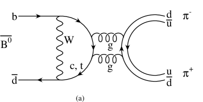
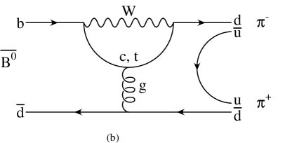
  Figure 4: (a) OZI-suppressed annihilation penguin diagram. This diagram is OZI-suppressed and is neglected within Assumption 4 because it does not contribute to $B\rightarrow K^{\pm}\pi^{\mp}$. (b) Non-OZI-suppressed annihilation penguin diagram. This diagram is not OZI-suppressed, although it has annihilation topology. It is not neglected within Assumption 4 because it contributes to both $B\rightarrow\pi^{+}\pi^{-}$ and $B\rightarrow K^{\pm}\pi^{\mp}$.

In particular, we do not neglect the electroweak penguin as it produces the same amplitude in $B\rightarrow K^{\pm}\pi^{\mp}$ and $B\rightarrow\pi^{+}\pi^{-}$, assuming SU(3) and neglecting OZI-suppressed penguins. Then we get simply from Eqs. (33), (38) and (40)

$$|P|=\left|\frac{V_{td}V_{tb}^{\ast}}{V_{cs}V_{cb}^{\ast}}\right|\times|P_{K^{+}\pi^{-}}|=\lambda\frac{\sin\gamma}{\sin\alpha}\,|P_{K^{+}\pi^{-}}|$$ (89)

where the geometry of the UT has been used in writing $|V_{td}/V_{cb}^{\ast}|$. From Eqs. (40) and (46), we get the following bound on $|P_{K^{+}\pi^{-}}|$:

$$|P_{K^{+}\pi^{-}}|^{2}\sin^{2}\gamma\,\leq\,{\cal B}_{K^{\pm}\pi^{\mp}}\,.$$ (90)

Combining it with Eqs. (60) and (89) we obtain 

$$|2\alpha-2\alpha_{\rm eff}|\leq\arccos\left[\frac{1}{\sqrt{1-a_{\rm dir}^{2}}}\left(1-2\lambda^{2}\,\frac{{\cal B}_{K^{\pm}\pi^{\mp}}}{{\cal B}_{\pi^{+}\pi^{-}}}\right)\right]\ \ \ \ \ \mbox{[assuming~{}{\bf 3} and~{}{\bf 4}].}$$ (91)

Thus this bound is a quantitative realization of the well-known fact that the penguin in $\pi\pi$ is $\lambda$-suppressed with respect to the penguin in $K\pi$: if $\lambda^{2}{\cal B}_{K^{\pm}\pi^{\mp}}/{\cal B}_{\pi^{+}\pi^{-}}$ is not too large, this means that the penguin cannot be too large in $B\rightarrow\pi\pi$. Note that similarly to the $B\rightarrow\pi^{0}\pi^{0}$ and $B\rightarrow K^{0}\overline{K^{0}}$ channels, we have not assumed penguin dominance in $B\rightarrow K\pi$ although of course the bound should be more interesting when the penguin amplitude really dominates in the latter decay.

From the experimental point of view, the bound that we have found in Eq. (91) should be considerably less affected by statistical uncertainties than the bounds (81), (83) and (87). Indeed, rather than measuring the branching ratio of very rare decays such as $B\rightarrow\pi^{0}\pi^{0}$ or $B\rightarrow K^{0}\overline{K^{0}}$, the use of the bound (91) needs to know ${\cal B}_{K^{\pm}\pi^{\mp}}$ which is ${\cal O}(10^{-5})$. For this reason the CLEO data (47) already help to give a very interesting and non trivial estimation of the r.h.s. of (91). Indeed (91) imply $|2\alpha-2\alpha_{\rm eff}|\leq\arccos(1-2\lambda^{2}{\cal B}_{K^{\pm}\pi^{\mp}}/{\cal B}_{\pi^{+}\pi^{-}})$ and from (47) we have $0.81\times 10^{-5}<{\cal B}_{K^{\pm}\pi^{\mp}}<2.0\times 10^{-5}$ and ${\cal B}_{\pi^{+}\pi^{-}}<0.84\times 10^{-5}$ at 90% C.L.. Assuming furthermore $0.4\times 10^{-5}<{\cal B}_{\pi^{+}\pi^{-}}$—otherwise the study of CP-violation in the $\pi\pi$ channel would be very difficult, independently of penguins—we obtain the bound

$$|2\alpha-2\alpha_{\rm eff}|\leq\Delta\,,\ \ \ \mbox{with}\ \ \ 25^{\circ}<\Delta<59^{\circ}\,.$$ (92)

Thus, although these data indicate that the extraction of $\alpha$ will not be an easy task, they are still compatible with a relatively small penguin-induced theoretical error. We would like to stress also that to our knowledge, this is the first time that a numerical upper bound on the theoretical error on $\alpha$ is given rather model-independently, with only mild theoretical assumptions and before the experimental value of $\alpha_{\rm eff}$ is available by itself. It is expected that experiment will give an accurate determination of the r.h.s. of (91) quite soon. Unless we are unlucky and ${\cal B}_{\pi^{+}\pi^{-}}$ is much smaller than expected, the theoretical errol on $\alpha$ constrained by the bound (91) should not excess $\sim 30^{\circ}$ while it can be as small as $\sim 10^{\circ}$. In comparison, the current knowledge of $\alpha$ is roughly $40^{\circ}<\alpha<140^{\circ}$ .

Finally one has again a bound independent of $a_{\rm dir}$ where $2\overline{\alpha}_{\rm eff}$ is involved:

$$|2\alpha-2\overline{\alpha}_{\rm eff}|\leq\arccos\left(1-2\lambda^{2}\,\frac{{\cal B}_{K^{\pm}\pi^{\mp}}}{{\cal B}_{\pi^{+}\pi^{-}}}\right)\ \ \ \ \ \mbox{[assuming~{}{\bf 3} and~{}{\bf 4}].}$$ (93)

Let us note in passing that the inequality (90), together with the assumption $|P_{K^{+}\pi^{-}}|^{2}=\mbox{{\rm BR}}(B^{\pm}\rightarrow K\pi^{\pm})\equiv{\cal B}_{K\pi^{\pm}}$ (that we will use in Section 6), leads to the Fleischer-Mannel bound on $\sin^{2}\gamma$ [22]. However, the bound (90) is exact independently of the assumption $|P_{K^{+}\pi^{-}}|^{2}={\cal B}_{K\pi^{\pm}}$.

5.3 Upper Bounds on $|2\alpha-2\alpha_{\rm eff}|$: Numerical Examples

In Appendix A, we define a typical set of parameters for the quantities involved in the channels that we are interested in. This set of parameters, compatible with the CLEO data (47), allows to compute the various observables (branching ratios and CP-asymmetries), and in particular to estimate numerically the bounds we have derived until now:

$$|2\alpha-2\alpha_{\rm eff}|\leq\arccos\left[\frac{1}{\sqrt{1-a_{\rm dir}^{2}}}\left(1-2\frac{{\cal B}_{\pi^{0}\pi^{0}}}{{\cal B}_{\pi^{\pm}\pi^{0}}}\right)\right]=33.4^{\circ}$$ (94)

$$|2\alpha-2\alpha_{\rm eff}|\leq\arccos\left[\frac{1}{\sqrt{1-a_{\rm dir}^{2}}}\left(1-4\frac{{\cal B}_{\pi^{0}\pi^{0}}}{{\cal B}_{\pi^{+}\pi^{-}}}\right)\right]=40.3^{\circ}$$ (95)

$$|2\alpha-2\alpha_{\rm eff}|\leq\arccos\left[\frac{1}{\sqrt{1-a_{\rm dir}^{2}}}\left(1-2\frac{{\cal B}_{K^{0}\overline{K^{0}}}}{{\cal B}_{\pi^{+}\pi^{-}}}\right)\right]=27.1^{\circ}$$ (96)

$$|2\alpha-2\alpha_{\rm eff}|\leq\arccos\left[\frac{1}{\sqrt{1-a_{\rm dir}^{2}}}\left(1-2\lambda^{2}\,\frac{{\cal B}_{K^{\pm}\pi^{\mp}}}{{\cal B}_{\pi^{+}\pi^{-}}}\right)\right]=29.9^{\circ}$$ (97)

The true value being $2\alpha-2\alpha_{\rm eff}=+26.7^{\circ}$ (Appendix A), the bound (96) is very close to be saturated for this set of parameters. Note also that the bounds (94-97) are numerically close one from one another, that just follows from our set of parameters and needs not to be true in general. As said above, it may happen in practice that the experiment gives only an upper bound on the suppressed channels ${\cal B}_{\pi^{0}\pi^{0}}$ and ${\cal B}_{K^{0}\overline{K^{0}}}$, in which case the bound (97) will certainly be more informative as ${\cal B}_{K^{\pm}\pi^{\mp}}$ is already measured and hopefully the ratio ${\cal B}_{K^{\pm}\pi^{\mp}}/{\cal B}_{\pi^{+}\pi^{-}}$ will be known with high accuracy very soon.

In any case and for the illustrative purpose, we will examine the case of the bound $|2\alpha-2\alpha_{\rm eff}|\leq 30^{\circ}$, which is in the ball-park of (94-97). On Fig. 5 we show the constraints of such a bound in the $(|P/T|,2\alpha)$ plane, and in the $(\rho,\eta)$ plane. The latter are obtained by plotting the circle defined by $2\alpha={\rm C^{st}}$, which equation is (cf. also Eq. (73)):

$$\left(\rho-\frac{1}{2}\right)^{2}+\left(\eta-\frac{\sin 2\alpha}{2(1-\cos 2\alpha)}\right)^{2}=\frac{1}{2(1-\cos 2\alpha)}\,.$$ (98)

We let $2\alpha$ vary in the interval $[2\alpha_{\rm eff}-30^{\circ},2\alpha_{\rm eff}+30^{\circ}]$ that is consistent with the bound.

  

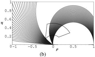
Figure 5: (a) The bound $|2\alpha-2\alpha_{\rm eff}|\leq\Delta$ in the $(|P/T|,2\alpha)$ plane, obtained as explained in the text, for the numerical example $a_{\rm dir}=0.12$, $\sin 2\alpha_{\rm eff}=0.58$ (see Appendix A) and $\Delta=30^{\circ}$ (solid curves limited by the small dashes). (b) The same bound in the $(\rho,\eta)$ plane, obtained by plotting the circle (98) for $2\alpha$ varying in the interval $[2\alpha_{\rm eff}-\Delta,2\alpha_{\rm eff}+\Delta]$. There are two families of circles corresponding to the two possible signs for $\cos 2\alpha_{\rm eff}$. In the background is shown a crude representation of the early-1998 allowed domain [32].

Thus the bounds (94-97) should give important and rather safe information on the angle $2\alpha$ as it is apparent on Fig. 5. Even if the penguin-induced error on $\alpha$ may be large, it is bounded by theoretical arguments, which is already an important statement in view of the possible tests of the consistency of the SM.

5.4 A Lower Bound on $|2\alpha-2\alpha_{\rm eff}|$ from $B\rightarrow K^{\pm}\pi^{\mp}$

It is clear from the examples in § 5.3 that a lower bound on $|2\alpha-2\alpha_{\rm eff}|$ would be a valuable information: it would permit to eliminate some region around $2\alpha=2\alpha_{\rm eff}$ and to get four separate intervals for $2\alpha$ (cf. Fig 1) instead of the two big ones represented on Fig. 5. Thus one may look for a lower bound on the absolute magnitude of the penguin. However, without any further theoretical assumptions (see Section 6), such a lower bound cannot be obtained using branching ratios only (for example the bound discussed in § 3.3 is not theoretically justified). Conversely, using direct CP-asymmetry in the $B^{\pm}\rightarrow K^{\pm}\pi^{\mp}$ decay, it is possible to get a lower bound on $|P|$, as well as a slightly improved upper bound with respect to the bound (91). The idea is the following: if a direct CP-asymmetry in the $B\rightarrow K^{\pm}\pi^{\mp}$ channel is detected, then it proves that this mode is fed by both tree and penguin contributions. As the latter is related by SU(3) to the penguin in the $B\rightarrow\pi^{+}\pi^{-}$ channel, and thus to the penguin-induced shift $|2\alpha-2\alpha_{\rm eff}|$, one gets a lower bound on this quantity .

Analogously to the derivation of Eq. (60), we get from Eq. (40)

$$2\,|P_{K^{+}\pi^{-}}|^{2}\sin^{2}\gamma=\left[1-\sqrt{1-\left[a_{\rm dir}^{K\pi}\right]^{2}}\cos\zeta\right]{\cal B}_{K^{\pm}\pi^{\mp}}$$ (99)

where

$${a_{\rm dir}^{K\pi}}=\frac{\mbox{{\rm BR}}(B^{0}\rightarrow K^{+}\pi^{-})-\mbox{{\rm BR}}(\overline{B^{0}}\rightarrow K^{-}\pi^{+})}{\mbox{{\rm BR}}(B^{0}\rightarrow K^{+}\pi^{-})+\mbox{{\rm BR}}(\overline{B^{0}}\rightarrow K^{-}\pi^{+})}$$ (100)

should be relatively easy to measure for this self-tagging mode, and $\zeta$ is a useful short-hand for the phase

$$\zeta=2\gamma-{\rm Arg}\left[A(B^{0}\rightarrow K^{+}\pi^{-})A^{\ast}(\overline{B^{0}}\rightarrow K^{-}\pi^{+})\right]\,.$$ (101)

Then, the inequality $|\cos\zeta|\leq 1$ together with Eqs. (89) and (99) imply

$$\lambda^{2}\left(1-\sqrt{1-\left[a_{\rm dir}^{K\pi}\right]^{2}}\right)\,{\cal B}_{K^{\pm}\pi^{\mp}}\,\leq\,2\,|P|^{2}\sin^{2}\alpha\,\leq\,\lambda^{2}\left(1+\sqrt{1-\left[a_{\rm dir}^{K\pi}\right]^{2}}\right)\,{\cal B}_{K^{\pm}\pi^{\mp}}$$ (102)

and from Eq. (60)

$$|2\alpha-2\alpha_{\rm eff}|\leq\arccos\left\{\frac{1}{\sqrt{1-a_{\rm dir}^{2}}}\left[1-\lambda^{2}\left(1+\sqrt{1-\left[a_{\rm dir}^{K\pi}\right]^{2}}\right)\,\frac{{\cal B}_{K^{\pm}\pi^{\mp}}}{{\cal B}_{\pi^{+}\pi^{-}}}\right]\right\}\,,$$ (103)

$$\arccos\left\{\frac{1}{\sqrt{1-a_{\rm dir}^{2}}}\left[1-\lambda^{2}\left(1-\sqrt{1-\left[a_{\rm dir}^{K\pi}\right]^{2}}\right)\,\frac{{\cal B}_{K^{\pm}\pi^{\mp}}}{{\cal B}_{\pi^{+}\pi^{-}}}\right]\right\}\leq|2\alpha-2\alpha_{\rm eff}|\,,$$ (104)

[assuming 3 and 4].

Note that if

$$\lambda^{2}\left(1-\sqrt{1-\left[a_{\rm dir}^{K\pi}\right]^{2}}\right)\,{\cal B}_{K^{\pm}\pi^{\mp}}\,\leq\,\left(1-\sqrt{1-a_{\rm dir}^{2}}\right)\,{\cal B}_{\pi^{+}\pi^{-}}$$ (105)

the SU(3) lower bound in (102) is useless as it is automatically verified thanks to Eq. (58) and the (exact) bound (63). Thus this lower bound is only useful in the configuration where the direct CP-asymmetry is very small in the $B\rightarrow\pi^{+}\pi^{-}$ channel ($a_{\rm dir}\rightarrow 0$) but large in the $B\rightarrow K^{\pm}\pi^{\mp}$ one (it becomes trivial in the limit $a_{\rm dir}^{K\pi}\rightarrow 0$), in which case the inequality (105) is not verified. As an example, it can be checked that the set of parameters defined in Appendix A verifies (105). However, keeping the same branching ratios and choosing the parameters such as $a_{\rm dir}=0$ and $a_{\rm dir}^{K\pi}=0.5$, the bound (104) is not trivial:

$$8^{\circ}\leq|2\alpha-2\alpha_{\rm eff}|\,,$$ (106)

while the bound (103) represents only a tiny improvement over (91).

Actually, one easily obtains similar lower bounds from the two previously studied channels, namely $B\rightarrow\pi^{0}\pi^{0}$, $B\rightarrow K^{0}\overline{K^{0}}$. However, the experimental detection of direct CP-violation in these suppressed channels may be a difficult task. Should it be feasible, one may do the full Gronau-London and/or Buras-Fleischer analyses (see Section 7).

6 Using the $B^{\pm}\rightarrow K\pi^{\pm}$ Decay to Determine $R_{P}$ with Further Assumptions

In this section, in addition to the hypothesis made in § 5.2 (Assumptions 3 and 4), we will assume more specifically that the two following approximations hold (to an accuracy to be determined) in Eqs. (40-41):

• Isospin symmetry and neglect of electroweak penguin contributions in $B\rightarrow K^{\pm}\pi^{\mp},K\pi^{\pm}$ (Assumptions 2 and 5). Note that the isospin symmetry is a consequence of the already assumed larger SU(3) symmetry. Neglecting the electroweak penguin, which is here colour-suppressed [28], we are allowed to write $P_{K^{+}\pi^{-}}=-P_{K^{0}\pi^{+}}$ [13].

• Neglect of the $V_{us}V_{ub}^{\ast}$ contribution to the $B^{+}\rightarrow K^{0}\pi^{+}$ amplitude (Assumption 6). That is, $T_{K^{0}\pi^{+}}=0$. Using a diagrammatic decomposition of the amplitude , we have $T_{K^{0}\pi^{+}}=|V_{us}V_{ub}^{\ast}|(M_{a}+M_{u}-M_{t})$ and $P_{K^{0}\pi^{+}}=|V_{cs}V_{cb}^{\ast}|(M_{c}-M_{t})$, where $M_{a}$ is the tree annihilation amplitude and $M_{u}$ (resp. $M_{c}$ resp. $M_{t}$) is the $u$- (resp. $c$- resp. $t$-) penguin. Note that $T_{K^{0}\pi^{+}}$ is suppressed by $|V_{us}V_{ub}^{\ast}|/|V_{cs}V_{cb}^{\ast}|\sim 2\times 10^{-2}$ compared to the dominant amplitude $P_{K^{0}\pi^{+}}$. Thus we have presumably $|V_{us}V_{ub}^{\ast}||M_{u}-M_{t}|\ll|V_{cs}V_{cb}^{\ast}||M_{c}-M_{t}|$, and it is often assumed that annihilation processes are negligible due to form-factor suppression [6], which then lead to $|T_{K^{0}\pi^{+}}|\ll|P_{K^{0}\pi^{+}}|$.

It is clear that Assumption 6 is on weaker grounds than the others made until now . Accepting it nevertheless, one is lead to many applications [6, 8] among which the most recent one is the Fleischer-Mannel bound [22]

$$\sin^{2}\gamma\,\leq\,\frac{{\cal B}_{K^{\pm}\pi^{\mp}}}{{\cal B}_{K\pi^{\pm}}}\,.$$ (107)

The latter has been recently questioned [31]. The problem is that FSI effects may invalidate the notion of colour-suppression for the electroweak penguin, thus leading to $P_{K^{+}\pi^{-}}\neq-P_{K^{0}\pi^{+}}$ [30]. Furthermore, the same effects may enhance annihilation diagrams, involving a significant $V_{us}V_{ub}^{\ast}$ contribution to $B^{+}\rightarrow K^{0}\pi^{+}$ and a possibly measurable direct CP-asymmetry in this channel [31]. We will not discuss this subject here. Rather we stress as previous authors that the $B\rightarrow K\overline{K}$ decays may help in constraining the FSI effects [20, 34]. In particular, the very easy to detect $B\rightarrow K^{+}K^{-}$ mode is fed only by annihilations diagrams. CLEO has already given an interesting bound on its branching ratio [16]:

$${\cal B}_{K^{+}K^{-}}<0.24\times 10^{-5}\ \ \ \ \ \ \ \mbox{[90\% C.L.].}$$ (108)

Thus, either the FSI effects are non-negligible and the $K^{+}K^{-}$ final state should be detected very soon, or they are eventually out of reach of experiment and a stringent bound on ${\cal B}_{K^{+}K^{-}}$ should be obtained [34]. As claimed by the authors of Refs. [31], FSI effects may easily invalidate the bound (107); indeed, to get a significant constraint on $\gamma$, we need the ratio ${\cal B}_{K^{\pm}\pi^{\mp}}/{\cal B}_{K\pi^{\pm}}$ to be sufficiently less than 1  in order to be not too much affected by a reasonable theoretical uncertainty induced by the neglect of electroweak penguin and annihilation contributions. On the contrary, for the case we are interested in, namely the extraction of $\alpha$, we do not need ${\cal B}_{K^{\pm}\pi^{\mp}}/{\cal B}_{K\pi^{\pm}}\leq 1$, and we will see that even in the presence of a sizeable violation of the above assumptions, we can get interesting information in the $(\rho,\eta)$ plane. In other words our method concerning $\alpha$ is useful whatever the values of the branching ratios are. However the Fleischer-Mannel bound is not affected by SU(3) breaking, while our method is. Note also that Fleischer [20] and Gronau [34] have proposed very recently extensive methods which may help to control FSI and electroweak penguin effects for the extraction of $\gamma$.

Returning to the problem of $\alpha$, we use the above hypotheses to write $|P_{K^{+}\pi^{-}}|=|P_{K^{0}\pi^{+}}|=|A(B^{+}\rightarrow K^{0}\pi^{+})|=|A(B^{-}\rightarrow\overline{K^{0}}\pi^{-})|$ and thus (recall the notations (33), (38), (40-41))

$$R_{P}\equiv|\lambda V_{cb}|^{2}\frac{|M^{(t)}|^{2}}{{\cal B}_{\pi^{+}\pi^{-}}}=\lambda^{2}\frac{{\cal B}_{K\pi^{\pm}}}{{\cal B}_{\pi^{+}\pi^{-}}}\ \ \ \ \ \mbox{[assuming~{}{\bf 3},~{}{\bf 4},~{}{\bf 5} and~{}{\bf 6}].}$$ (109)

The above determination of $R_{P}$ can be used to insert in Eq. (72). Of course, the reader who does not agree with the assumptions leading to Eq. (109) can use its own model to estimate $R_{P}$. Thus the method described here is very general, and is in any case weakly model-dependent as it depends on only one estimated parameter. The results shown below in the $(\rho,\eta)$ plane are quite typical of what can be obtained with such a method.

However, at this stage there is still a problem in using Eq. (109): it is clear that we have to give a theoretical error associated with the above determination of the penguin amplitude. As a guess, we will simply allow a relative violation of Eq. (109) of the order of 30% and 60% respectively (at the amplitude level), and leave for the future any justification of these values. Actually, as long as this error is less than 100%, the method described here is more powerful than the bounds derived in the previous sections .

On Fig. 6 we solve Eq. (72) with the theoretical input (109), and with the numerical values obtained in Appendix A. Note that with our set of parameters, the Fleischer-Mannel bound becomes trivial ($\sin^{2}\gamma\leq 1$) but it does not prevent to get useful results from Eq. (72). Fig. 6 shows that with a reasonable 30% relative violation of the theoretical assumptions (at the amplitude level) leading to Eq. (109), the time-dependent $B\rightarrow\pi\pi$ CP-asymmetry defines a small allowed domain in the $(\rho,\eta)$ plane, much more informative than the more conservative bounds derived in the previous sections. This statement is quite general: if there is a way to estimate the parameter $|P/T|$ (or $|P|$ or $R_{P}/R_{T}$ or $R_{P}$) with an uncertainty of order $\sim 30\%$, then Eq. (58) (or Eq. (60) or Eq. (71) or Eq. (72)) will give rather strong constraints on $\alpha$ (or on the allowed domain in the $(\rho,\eta)$ plane). We will see in § 7.1 and 7.2 that the isospin analysis is not much more better in this respect because it is plagued by more discrete ambiguities. Finally we stress that from the experimental point of view, our proposal is very favourable: in addition to the usual time-dependent $B^{0}(t)\rightarrow\pi^{+}\pi^{-}$ CP-asymmetry, our analysis require only the measurement of the $B^{\pm}\rightarrow K\pi^{\pm}$ average branching ratio, which is already measured (cf. Eq. (47)). In this sense our proposal represents an improvement with respect to the Fleischer-Mannel’s [8], because the latter needs the further knowledge of ${\cal B}_{\pi^{\pm}\pi^{0}}$ and $|V_{td}|$ (cf. § 7.4).

  

Figure 6: The solutions of the degree-four polynomial equation (72) in the $(\rho,\eta)$ plane for the numerical example $a_{\rm dir}=0.12$, $\sin 2\alpha_{\rm eff}=0.58$ and $R_{P}=\lambda^{2}{\cal B}_{K\pi^{\pm}}/{\cal B}_{\pi^{+}\pi^{-}}=0.061$ (see Appendix A). A guess value for the relative theoretical uncertainty on $R_{P}$ in Eq. (109) is assumed: respectively 30% (a) and 60% (b), at the amplitude level. There are four families of curves corresponding to the two possible signs for $\cos 2\alpha_{\rm eff}$, and to the cosine discrete ambiguity of Eq. (60) which is hidden in the polynom (72). In the background is shown a crude representation of the early-1998 allowed domain [32].

7 Recovering and Improving some of the Previous Approaches

In this section, we will explain how to recover in our language the Gronau-London [4], the Buras-Fleischer [7], the Fleischer-Mannel [8] and the Marrocchesi-Paver [11] proposals, and in some places we will propose improvements of these methods.

7.1 The Gronau-London Isospin Analysis

Gronau and London have proposed a clean method to get rid of the penguin-induced shift on $\alpha$ [4, 13] by measuring all the $B\rightarrow\pi\pi$ branching ratios in addition to the time-dependent CP-asymmetry (30). Rather than repeating the geometrical demonstration contained in the original paper, we give here the equivalent analytical formulæ and show the isospin construction in the $\left(|P/T|,2\alpha\right)$ plane.

The Gronau-London method relies on the isospin symmetry of the strong interactions: after having defined

$$\Phi \equiv {\rm Arg}\left(A_{\pi^{+}\pi^{0}}A^{\ast}\right)\,,$$ (110)

$$\overline{\Phi} \equiv {\rm Arg}\left(\bar{A}_{\pi^{-}\pi^{0}}\bar{A}^{\ast}\right)\,,$$ (111)

simple trigonometry in Eqs. (76-78) gives:

$$\cos\Phi = \frac{1}{\sqrt{2}|A||A_{\pi^{+}\pi^{0}}|}\left[\frac{1}{2}|A|^{2}+|A_{\pi^{+}\pi^{0}}|^{2}-|A_{\pi^{0}\pi^{0}}|^{2}\right]\,,$$ (112)

$$\cos\overline{\Phi} = \frac{1}{\sqrt{2}|\bar{A}||\bar{A}_{\pi^{-}\pi^{0}}|}\left[\frac{1}{2}|\bar{A}|^{2}+|\bar{A}_{\pi^{-}\pi^{0}}|^{2}-|\bar{A}_{\pi^{0}\pi^{0}}|^{2}\right]\,.$$ (113)

Eqs. (112-113) are not yet sufficient to trap the penguin. However, setting $P_{\rm EW}=0$ in (78) implies ${\rm Arg}\left(\frac{q}{p}\bar{A}_{\pi^{-}\pi^{0}}A_{\pi^{+}\pi^{0}}^{\ast}\right)=2\alpha$ and thus

$$2\alpha=2\alpha_{\rm eff}+\overline{\Phi}-\Phi\,.$$ (114)

To summarize, measuring the $B\rightarrow\pi\pi$ branching ratios allows to extract the angles $\Phi$ and $\overline{\Phi}$ (up to a fourfold discrete ambiguity which corresponds to the four possible orientations of the Gronau-London triangle [4, 13]) thanks to Eqs. (112-113). As the CP-asymmetry gives $2\alpha_{\rm eff}$ up to a twofold discrete ambiguity, it is possible to get $2\alpha$ and $|P/T|$ from Eqs. (114) and (58) up to an eightfold discrete ambiguity, as Fig. 7 shows.

  

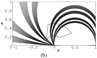
Figure 7: The eight solutions of the Gronau-London isospin analysis, for the numerical example $a_{\rm dir}=0.12$, $\sin 2\alpha_{\rm eff}=0.58$, ${\cal B}_{\pi^{\pm}\pi^{0}}/{\cal B}_{\pi^{+}\pi^{-}}=0.71$, ${\cal B}_{\pi^{0}\pi^{0}}/{\cal B}_{\pi^{+}\pi^{-}}=0.061$ and a direct CP-asymmetry in the $\pi^{0}\pi^{0}$ channel equal to $a_{\rm dir}^{\pi^{0}\pi^{0}}=0.32$ (see Appendix A). (a) In the $(|P/T|,2\alpha)$ plane, the dots represent the central values obtained from Eqs. (112-114), while the solid curves (limited by the small dashes) represent the allowed domain when assuming that $2\alpha$ is affected by a $4^{\circ}$ uncertainty due to electroweak penguin contributions, as explained in the text. (b) The same allowed domain is represented in the $(\rho,\eta)$ plane, where it is obtained by plotting the circle (98) for $2\alpha$ varying in the eight solution intervals. In the background is shown a crude representation of the early-1998 allowed domain [32].

Let us show explicitly that expressing the problem in terms of $\sin 2\alpha$ is somewhat misleading: from Fig. 7, we can plot the eight solutions of the isospin analysis in the $(|P/T|,\sin 2\alpha)$ plane, as showed in Fig. 8(a).

  

Figure 8: (a) The eight solutions of the isospin analysis in the $(|P/T|,\sin 2\alpha)$ plane, for the same observables as in Fig. 7. (b) The solutions in the $(|P/T|,2\alpha)$ plane obtained by computing $\arcsin(\sin 2\alpha)$ and $\pi-\arcsin(\sin 2\alpha)$: the comparison with Fig. 7 shows that the crosses are wrong solutions.

Now if we forget Fig. 7 and try to get the solutions in $2\alpha$ from Fig. 8(a), we obtain the sixteen solutions of Fig. 8(b), among which eight are obviously wrong. Note two important points which have been mistreated in the original paper [4] and to our knowledge in the subsequent literature: First, there are eight solutions in terms of $2\alpha$ and also in terms of $\sin 2\alpha$  . Second, the isospin analysis determines $2\alpha$ rather than $\sin 2\alpha$.

7.2 Defining the Error Due to the Electroweak Penguin

One may wonder on the size of the electroweak penguin, which is neglected in the isospin analysis. Several authors have estimated this contribution, which turns out to be a few percents of the dominant $B\rightarrow\pi^{+}\pi^{-}$ amplitude [28, 29]. If this estimation is correct, then the corresponding uncertainty on $\alpha$ may be a few degrees, which is negligible compared to the most optimistic simulations of the statistical uncertainty  [26]. In any case, a simple parametrization of the electroweak penguin effects can be obtained: indeed, when $P_{\rm EW}\neq 0$, there are two new parameters, namely ${\rm Arg}(P_{\rm EW}T^{\ast})$ and $|P_{\rm EW}|$, and one new observable which is the direct CP-asymmetry in the $B^{\pm}\rightarrow\pi^{\pm}\pi^{0}$ channel

$$a_{\rm dir}^{\pi^{\pm}\pi^{0}}=\frac{\mbox{{\rm BR}}(B^{+}\rightarrow\pi^{+}\pi^{0})-\mbox{{\rm BR}}(B^{-}\rightarrow\pi^{-}\pi^{0})}{\mbox{{\rm BR}}(B^{+}\rightarrow\pi^{+}\pi^{0})+\mbox{{\rm BR}}(B^{-}\rightarrow\pi^{-}\pi^{0})}$$ (115)

which vanishes when $P_{\rm EW}\rightarrow 0$. Similarly to the case of the strong penguin, as discussed at length in this paper, it is possible to express $\alpha$ as a simple function of the observables of the Gronau-London isospin analysis, the direct CP-asymmetry in the $B^{\pm}\rightarrow\pi^{\pm}\pi^{0}$ channel and the unknown parameter $|P_{\rm EW}|$. The same technique leading to Eq. (58) allows to find

$$\cos(2\alpha-2\alpha^{\prime}_{\rm eff})=\frac{1}{\sqrt{1-\left[a_{\rm dir}^{\pi^{\pm}\pi^{0}}\right]^{2}}}\left[1-\left(1-\sqrt{1-\left[a_{\rm dir}^{\pi^{\pm}\pi^{0}}\right]^{2}}\cos 2\alpha^{\prime}_{\rm eff}\right)\left|\frac{P_{\rm EW}}{T_{\pi^{+}\pi^{0}}}\right|^{2}\right]$$ (116)

where $2\alpha^{\prime}_{\rm eff}$ is the value of $2\alpha$ when $P_{\rm EW}=0$ (see Eq. (114))

$$2\alpha^{\prime}_{\rm eff}=2\alpha_{\rm eff}+\overline{\Phi}-\Phi\,.$$ (117)

Thus Eqs. (116-117) describe the departure from the isospin analysis (114) due to the electroweak penguin contributions. As a particular case, we obtain the bound

$$|2\alpha-2\alpha^{\prime}_{\rm eff}|\leq\arccos\left[1-2\left|\frac{P_{\rm EW}}{T_{\pi^{+}\pi^{0}}}\right|^{2}\right]\sim 2\left|\frac{P_{\rm EW}}{T_{\pi^{+}\pi^{0}}}\right|$$ (118)

which was derived in Ref. [28]. Note that the ratio $|P_{\rm EW}/T_{\pi^{+}\pi^{0}}|$ is rather independent of the size of the colour-suppression, although the impact of $|P_{\rm EW}|$ on BR$(B\rightarrow\pi^{0}\pi^{0})$ is not negligible.

Thus, whatever the way to estimate the parameter $|P_{\rm EW}/T_{\pi^{+}\pi^{0}}|$, one is lead to a simple and weakly model-dependent definition of the theoretical error on $\alpha$ induced by the electroweak penguin. Using factorization for the estimation of the r.h.s. of (118), we find typically $|2\alpha-2\alpha^{\prime}_{\rm eff}|{~{}\raise 1.49994pt\hbox{$<$}\kern-8.50006pt\lower 3.50006pt\hbox{$\sim$}~{}}4^{\circ}$; this error has been reported on Fig. 7 for illustration. This figure shows the sensitivity of the isospin analysis with respect to the discrete ambiguities: with an error on $\alpha$ as small as $2^{\circ}$ (here this error comes from the electroweak penguin contributions, but unfortunately there are also the uncertainties of experimental origin which we have not considered), the four separate solutions (for a given sign of $\cos 2\alpha_{\rm eff}$) tends to merge quite quickly. This is not a posteriori surprising: indeed these four solutions are separated because of the QCD penguin contributions, i.e. because of a relatively small effect; they become degenerate in the no-penguin limit. Comparison with Figs. 5 and 6 suggests actually that the more simpler approaches to control the penguin effects described in the previous sections may be competitive with the more complete isospin analysis, unless the observables of the latter are known with a very high accuracy.

The main drawback of the Gronau-London analysis is the expected rarity of the $B\rightarrow\pi^{0}\pi^{0}$ channel, which branching ratio is expected to be about $10^{-7}$–$10^{-6}$. The neutral pions are not easy to detect, and one needs to tag the flavour of the $B$-meson in order to get separately $|A_{\pi^{0}\pi^{0}}|$ and $|\bar{A}_{\pi^{0}\pi^{0}}|$, according to Eqs. (112-113). The small number of effectively useful events expected at an $e^{+}e^{-}$ $B$-factory constitutes a difficult challenge to the experimentalists while the impossibility to detect two neutral pions in future hadronic machines does not improve the situation. This shows the interest of the bounds (81) and (83).

7.3 The Buras-Fleischer Proposal

Considering the experimental difficulties associated with the Gronau-London analysis, Buras and Fleischer have proposed an alternative way to get rid of the penguin uncertainty, using SU(3) and the time-dependent CP-asymmetry of the pure penguin mode $B\rightarrow K^{0}\overline{K^{0}}$  [7]. They argue that the SU(3) breaking effects are of the same order as the electroweak penguin uncertainty of the isospin analysis.

The idea is simple: similarly to the $B\rightarrow\pi^{+}\pi^{-}$ decay we define the time-dependent $B\rightarrow K^{0}\overline{K^{0}}$ CP-asymmetry

$$a^{K\bar{K}}_{\rm CP}(t)=a_{\rm dir}^{K\bar{K}}\cos\Delta m\,t-\sqrt{1-\left[a_{\rm dir}^{K\bar{K}}\,\right]^{2}}\sin 2\alpha_{\rm eff}^{K\bar{K}}\sin\Delta m\,t\,,$$ (119)

where we have used the notation $\sin 2\alpha_{\rm eff}^{K\bar{K}}$ to make apparent the resemblance with Eq. (30): we stress however that $2\alpha_{\rm eff}^{K\bar{K}}$ reduces to $2\alpha$ when the $T_{K\overline{K}}$ amplitude dominates in Eq. (39), i.e. when the difference between the $u$- and $c$- penguins dominates over the difference between the $t$- and $c$- penguins, which is presumably an extreme case. Conversely, in the absence of long-distance $u$- and $c$- penguins, we have $\sin 2\alpha_{\rm eff}^{K\bar{K}}=a_{\rm dir}^{K\bar{K}}=0$ [21, 7].

Thus, following Eq. (60) we find

$$|P_{K^{0}\overline{K^{0}}}|^{2}=\frac{{\cal B}_{K^{0}\overline{K^{0}}}}{1-\cos 2\alpha}\left[1-\sqrt{1-\left[a_{\rm dir}^{K\bar{K}}\,\right]^{2}}\cos(2\alpha-2\alpha_{\rm eff}^{K\bar{K}})\right]\,,$$ (120)

which reduces to $|P_{K^{0}\overline{K^{0}}}|^{2}={\cal B}_{K^{0}\overline{K^{0}}}$ if the top-penguin dominates the amplitude.

Assuming SU(3) and neglecting the (colour-suppressed) electroweak penguin contributions, we may write

$$|P|=|P_{K^{0}\overline{K^{0}}}|\,.$$ (121)

Thus from Eqs. (60), (120) and (121) we have

$$\left[1-\sqrt{1-a_{\rm dir}^{2}}\cos(2\alpha-2\alpha_{\rm eff})\right]-\frac{{\cal B}_{K^{0}\overline{K^{0}}}}{{\cal B}_{\pi^{+}\pi^{-}}}\left[1-\sqrt{1-\left[a_{\rm dir}^{K\bar{K}}\,\right]^{2}}\cos(2\alpha-2\alpha_{\rm eff}^{K\bar{K}})\right]=0\,.$$ (122)

Defining the following quantity that can be written in terms of observables

$${\cal D} = \sqrt{1-a_{\rm dir}^{2}}\,\exp(i\,2\alpha_{\rm eff})-\frac{{\cal B}_{K^{0}\overline{K^{0}}}}{{\cal B}_{\pi^{+}\pi^{-}}}\sqrt{1-\left[a_{\rm dir}^{K\bar{K}}\,\right]^{2}}\,\exp(i\,2\alpha_{\rm eff}^{K\bar{K}})$$ (123)

$$\equiv |{\cal D}|e^{i\Psi}\,,$$

Eq. (122) becomes

$$\cos(2\alpha-\Psi)=\frac{1}{|{\cal D}|}\left[1-\frac{{\cal B}_{K^{0}\overline{K^{0}}}}{{\cal B}_{\pi^{+}\pi^{-}}}\right]\,.$$ (124)

As $2\alpha_{\rm eff}$ and $2\alpha_{\rm eff}^{K\bar{K}}$ are both measured up to a twofold discrete ambiguity, Eq. (124) gives $2\alpha$ up to an eightfold discrete ambiguity. An explicit example is given on Fig. 9.

  

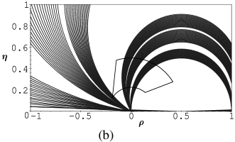
Figure 9: The eight solutions of the Buras-Fleischer analysis, for the numerical example $a_{\rm dir}=0.12$, $\sin 2\alpha_{\rm eff}=0.58$, $a_{\rm dir}^{K\bar{K}}=0.21$, $\sin 2\alpha_{\rm eff}^{K\bar{K}}=0.059$ and ${\cal B}_{K^{0}\overline{K^{0}}}/{\cal B}_{\pi^{+}\pi^{-}}=0.058$ (see Appendix A). (a) In the $(|P/T|,2\alpha)$ plane, the dots represent the central values obtained from Eqs. (123-124), while the solid curves (limited by the small dashes) represent the allowed domain when assuming that Eq. (121) is affected by a guess 30% relative uncertainty. Some of the solutions merge because of this theoretical error, leaving only six separate solutions. (b) The same allowed domain is represented in the $(\rho,\eta)$ plane, where it is obtained by plotting the circle (98) for $2\alpha$ varying in the six solution intervals. In the background is shown a crude representation of the early-1998 allowed domain [32].

However from the experimental point of view the study of this decay may be as difficult as the isospin analysis: First, it is a pure $b\rightarrow d$ penguin decay and is thus expected to be very rare ($\sim 10^{-7}$–$10^{-6}$) [19]. And second, the time-dependence of the decay rate may be difficult to reconstruct because the neutral kaons decay far away from the primary vertex. This shows the interest of the bound (87), very symmetrically to the case of the isospin analysis.

7.4 The Fleischer-Mannel and Marrocchesi-Paver Methods

Fleischer and Mannel [8], as well as Marrocchesi and Paver [11] had already remarked that knowing the value of $|P/T|$ alone leads to the extraction of $\alpha$. Therefore they have used Eq. (58) without explicitly having written it, and without having noticed the complete generality of the method. Let us briefly sketch the main points of their studies:

• Fleischer and Mannel use a first-order expansion in $|P/T|$. We have shown that this approximation, although numerically good, is unnecessary: Eq. (58) is exact and not more complicated than its first-order expansion.

• Fleischer and Mannel estimate $|P/T|$ by assuming Eq. (109) and neglecting the colour-suppressed contributions to $B^{\pm}\rightarrow\pi^{\pm}\pi^{0}$ [8]

  $$\left|\frac{P}{T}\right|^{2}=\left|\frac{V_{td}V_{tb}^{\ast}}{V_{cs}V_{cb}^{\ast}}\right|^{2}\times\frac{{\cal B}_{K\pi^{\pm}}}{2{\cal B}_{\pi^{\pm}\pi^{0}}}\,,$$ (125)

  while Marrocchesi and Paver use factorization to calculate (in this case $|P/T|$ is just proportional to a ratio of short-distance Wilson coefficients times a CKM factor) [11]

  $$\left|\frac{P}{T}\right|=\frac{\sin(\alpha+\beta)}{\sin\beta}\times 0.055\,.$$ (126)

  The two above equations represent alternatives to the method presented in Section 6, although in the second case it is not clear to what extent factorization can be used to calculate $|P/T|$ [19]. Note that these two approaches use a single model-dependent input, as the method we have proposed in Section (6).

• Both Fleischer and Mannel and Marrocchesi and Paver face the problem of knowing $|V_{td}|$ or $\sin(\alpha+\beta)/\sin\beta$. The first two authors assume simply that $|V_{td}/(\lambda V_{cb})|$ is known from CP-conserving measurements [8], while the second two authors take the value of $\beta$ as it would be given by the future measurements of the $B\rightarrow J/\Psi K_{S}$ CP-asymmetry and obtain an equation depending on $\alpha$ alone [11]. However it is not clear if CP-conserving measurements will give $|V_{td}/(\lambda V_{cb})|$ with enough accuracy, and using instead the value of $\beta$ unfortunately propagates the uncertainty and the discrete ambiguities associated with the measurement of $\beta$ into the extraction of $\alpha$. We have shown in § 3.6 that one can avoid these problems by directly writing easy-to-solve polynomial equations in the $(\rho,\eta)$ plane, therefore without invoking other independent CKM measurements. For the Fleischer-Mannel proposal one should write $|P/T|^{2}=\lambda^{2}|1-\rho-i\eta|^{2}\times{\cal B}_{K\pi^{\pm}}/(2{\cal B}_{\pi^{\pm}\pi^{0}})$ and report this expression into Eq. (58) to obtain an equation  in the variables $(\rho,\eta)$, without the need to know $|V_{td}/(\lambda V_{cb})|$. For the Marrocchesi-Paver method one should simply insert $R_{P}/R_{T}=0.055$ in Eq. (71) independently of $\beta$. Thus our framework allows to improve significantly these proposals.

• Finally we would like to stress once again the importance of the discrete ambiguities. While they are not discussed at all by Fleischer and Mannel [8], we believe that the treatment of Marrocchesi and Paver is incomplete: for a given value of $|P/T|$ (inferred from factorization and a given value for $\beta$), they find two solutions for $\alpha$ between 0 and $\pi$. We have shown in § 3.4 that there are four such solutions which, because of the finiteness of the errors (both theoretical and experimental), may merge among themselves.

8 Conclusion

We have shown that in the presence of penguin contributions, the information on the CKM angle $\alpha$ coming from the measurement of the time-dependent $B^{0}(t)\rightarrow\pi^{+}\pi^{-}$ CP-asymmetry can be summarized in a set of simple equations, expressing $\alpha$ as a multi-valued function of a single theoretically unknown parameter. These equations, free of any assumption besides the Standard Model, provide by themselves an exact model-independent interpretation of future CP-experiments.

It is also possible to choose as the unknown a pure QCD quantity, in which case the above equations should be expressed directly in the $(\rho,\eta)$ plane, thanks to the unitarity of the CKM matrix which predicts relations between the CP-violating angles and the CP-conserving sides of the Unitarity Triangle. Whatever the choice of the single unknown, as for example the ratio of penguin to tree matrix elements, this unavoidable non-perturbative parameter in $B\rightarrow\pi^{+}\pi^{-}$ could be compared to $B_{K}$ in the kaon system which allows to report the measurement of $\epsilon_{K}$ in the $(\rho,\eta)$ plane. However the ratio $|P/T|$ is a much more complicated quantity than $B_{K}$, and would be very difficult to obtain from QCD fundamental methods.

Using these analytic expressions, we have assumed some reasonable hypotheses to constrain the free parameter. Doing so we have derived several new bounds on the penguin-induced shift $|2\alpha-2\alpha_{\rm eff}|$, generalizing the result of Grossman and Quinn [15]. One of these bounds is determined by the ratio $\lambda^{2}{\cal B}_{K^{\pm}\pi^{\mp}}/{\cal B}_{\pi^{+}\pi^{-}}$ on which one would have an experimental value very soon.

Accepting less conservative assumptions, stronger constraints on $\alpha$ can be obtained. For example in the limit where the annihilation and electroweak penguin diagrams can be neglected, and using SU(3), the knowledge of the $B^{\pm}\rightarrow K\pi^{\pm}$ branching ratio is a sufficient information to extract the theoretical unknown. Assuming a reasonable 30% relative uncertainty (at the amplitude level) on the unavoidable hypotheses, a relatively small allowed domain in the $(\rho,\eta)$ plane can be found, independently of any other measurement. This method could be competitive with the full Gronau-London isospin analysis, because the latter is plagued by twice more discrete ambiguities. From the experimental point of view, our proposal may be much more easier to achieve. More generally, if by some other argument a knowledge of the modulus of the penguin amplitude—or the ratio of penguin to tree—with a $\sim 30\%$ uncertainty can be achieved, then rather strong constraints on $\alpha$ should be obtained.

However we do not pretend that the theoretical uncertainty on $\alpha$ will be small. Rather we believe that this error may be quite well controlled by conservative arguments. This shows the importance of generalizing our framework to other channels sensitive to $\alpha$: if we are unlucky in the $\pi^{+}\pi^{-}$ channel, it may happen that we are lucky in others. As the problem of the discrete ambiguities is crucial in these analyses, the modes providing new CP-observables are of a particular interest: for example measuring directly the sign of $\cos 2\alpha_{\rm eff}$ rather than determining it from the SM constraints on the UT would be a valuable information, even in the presence of sizeable penguin contributions, as it would allow to reduce the discrete ambiguities generated when expressing $\alpha$ as a function of the observables and of one model-dependent input. It has been shown previously [36] that the analysis of the $B\rightarrow\rho\pi\rightarrow 3\pi$ Dalitz plot actually leads to the measurement of a kind of $\cos 2\alpha_{\rm eff}$  (which is of course different from the $\alpha_{\rm eff}$ in $B\rightarrow\pi\pi$), and we are currently studying the possibility to describe this interesting decay similarly to $B\rightarrow\pi\pi$ [37]. Likewise the angular distribution of the decay $B\rightarrow\Lambda\overline{\Lambda}$ contains also terms proportional to the cosine of an effective $\alpha$ angle [38].

It is quite clear that all the strategies proposed until now to disentangle the penguin pollution in various channels will give different information on $\alpha$, each relying on very different theoretical assumptions and on different observables. Our framework allows to treat all these sources of information in a transparent and unified way. Thus we will have certainly a strong cross-check of the various results. If this cross-check is successful, we may think to combine these results in order to have a more precise knowledge of $\alpha$. However, we are aware that combining theoretical and experimental errors is a difficult problem by itself which is beyond the scope of the present paper.

Appendix A A Typical Set of Theoretical Parameters

In this appendix, we define a typical set of parameters in order to compute the relevant observables. We assume that 1–6 are exact, and neglect further all annihilation diagrams. Thus the amplitudes in Eqs. (33-35), (39-41) write:

$$A(B^{0}\rightarrow\pi^{+}\pi^{-}) = e^{i\gamma}\,T+e^{-i\beta}\,P\,,$$ (127)

$$A(B^{0}\rightarrow\pi^{0}\pi^{0}) = \frac{1}{\sqrt{2}}\left[e^{i\gamma}\left(T-T_{\pi^{+}\pi^{0}}\right)-e^{-i\beta}\,P\right]\,,$$ (128)

$$A(B^{+}\rightarrow\pi^{+}\pi^{0}) = \frac{1}{\sqrt{2}}e^{i\gamma}\,T_{\pi^{+}\pi^{0}}\,,$$ (129)

$$A(B^{0}\rightarrow K^{0}\overline{K^{0}}) = P\left(e^{-i\beta}+\left|\frac{V_{ub}^{\ast}}{V_{td}}\right|e^{i\gamma}\,r_{u}\right)\,,$$ (130)

$$A(B^{0}\rightarrow K^{+}\pi^{-}) = \lambda e^{i\gamma}\,T+\left|\frac{V_{ts}}{\lambda V_{td}}\right|e^{i(\delta^{\prime}-\delta)}P\,,$$ (131)

$$A(B^{+}\rightarrow K^{0}\pi^{+}) = \left|\frac{V_{ts}}{\lambda V_{td}}\right|e^{i\delta^{\prime}}P\,.$$ (132)

Note that in the strict SU(3) limit and neglecting annihilation diagrams, $\delta^{\prime}=\delta$.

${\cal B}_{\pi^{+}\pi^{-}}$ (normalization)	${\cal B}_{\pi^{0}\pi^{0}}$	${\cal B}_{\pi^{\pm}\pi^{0}}$	${\cal B}_{K^{0}\overline{K^{0}}}$	${\cal B}_{K^{\pm}\pi^{\mp}}$	${\cal B}_{K\pi^{\pm}}$
0.75	0.0455	0.533	0.0433	1.075	0.948

Table 1: The various average branching ratios (in units of $10^{-5}$) from our set of parameters. They are consistent with CLEO data (47).

$a_{\rm dir}$	$\sin 2\alpha_{\rm eff}$	$a_{\rm dir}^{\pi^{0}\pi^{0}}$	$a_{\rm dir}^{K^{0}\overline{K^{0}}}$	$\sin 2\alpha_{\rm eff}^{K^{0}\overline{K^{0}}}$	$a_{\rm dir}^{K^{\pm}\pi^{\mp}}$
0.117	0.579	0.317	0.209	0.0592	0.108

Table 2: The various CP-asymetries from our set of parameters.

Numerically, we take ${\cal B}_{\pi^{+}\pi^{-}}=0.75\times 10^{-5}$, which fixes the normalization of the amplitudes and choose $T$ real which fixes the origin of phases. Then we choose $|P/T|=0.25$ which is a quite sizeable value (cf. § 3.3) and $\delta=-15^{\circ}$ which is a large violation of naive factorization which gives $\delta=180^{\circ}$. The normalization is then given by $|T|=0.826\times\sqrt{10^{5}{\cal B}_{\pi^{+}\pi^{-}}}$ (in “units of two-body branching ratio”). We choose also $T_{\pi^{+}\pi^{0}}=1.25e^{-i7^{\circ}}\times|T|$ which takes into account the usual $a_{2}\sim 0.25$ colour-suppression factor and some FSI phases, $\delta^{\prime}=+20^{\circ}$, and $r_{u}=0.3e^{+i75^{\circ}}$ which is a ratio of long-distance over short-distance penguin matrix elements. For the CKM parameters, we have $\lambda=0.2205$ and take $\rho=0.10$, $\eta=0.34$ which is around the center of the early-1998 allowed domain ($\alpha=85.7^{\circ}$) [23]. The resulting values for the observables are summarized in Tables 1 and  2. Let us stress that these values are only indicative and that the real numbers may be very different. Our set of parameters results from a compromise between the need to take into account various effects in a more or less realistic way and the pedagogical needs (for example it is easier to discuss the number of discrete solutions when they are quite well separated, which is often not the case in practice). Finally we notice that the penguin-induced shift on $\alpha$ is quite large for this set of parameters: $2\alpha-2\alpha_{\rm eff}=+26.7^{\circ}$.

Appendix B Bounds Independent of Direct CP-Violation

Here our purpose is to derive bounds which are fully independent of $a_{\rm dir}$, and thus are not affected by the experimental uncertainty associated with the measurement of direct CP-violation [39]. As far as the bound (16) is concerned, a different demonstration has been given by Grossman and Quinn [15].

Consider the bounds (16-19): they all can be written

$$\frac{1-m}{\sqrt{1-a_{\rm dir}^{2}}}\,\leq\,\cos(2\alpha-2\alpha_{\rm eff})$$ (133)

where $m$ is a positive ratio of branching ratios and is expected to be smaller than 2 (otherwise the bound is useless). If $a_{\rm dir}$ is not known, then $2\alpha_{\rm eff}$ is not known either. Rather one gets from the $\sin\Delta m\,t$ term in (32) the effective angle

$$\sin 2\overline{\alpha}_{\rm eff}\equiv\sqrt{1-a_{\rm dir}^{2}}\sin 2\alpha_{\rm eff}\,.$$ (134)

Since $|\sin 2\overline{\alpha}_{\rm eff}|\leq|\sin 2\alpha_{\rm eff}|$ one has:

$$|\cos 2\alpha_{\rm eff}|\,\leq\,|\cos 2\overline{\alpha}_{\rm eff}|\,.$$ (135)

As the sign of $\cos 2\overline{\alpha}_{\rm eff}$ is not observable, it can be chosen arbitrarily. It is convenient to define

$${\rm sign}(\cos 2\overline{\alpha}_{\rm eff})\equiv{\rm sign}(\cos 2\alpha)\,,$$ (136)

in such a way that (135) gives

$$|\cos 2\alpha_{\rm eff}\cos 2\alpha|\,\leq\,|\cos 2\overline{\alpha}_{\rm eff}\cos 2\alpha|=\cos 2\overline{\alpha}_{\rm eff}\cos 2\alpha\,.$$ (137)

Thus Eqs. (133) and (137) imply

$$1-m \leq \sqrt{1-a_{\rm dir}^{2}}\cos 2\alpha_{\rm eff}\cos 2\alpha+\sin 2\overline{\alpha}_{\rm eff}\sin 2\alpha$$ (138)

$$\leq |\cos 2\alpha_{\rm eff}\cos 2\alpha|+\sin 2\overline{\alpha}_{\rm eff}\sin 2\alpha$$

$$\leq \cos 2\overline{\alpha}_{\rm eff}\cos 2\alpha+\sin 2\overline{\alpha}_{\rm eff}\sin 2\alpha=\cos(2\alpha-2\overline{\alpha}_{\rm eff})\,,$$

and we obtain the announced result, namely

$$\frac{1-m}{\sqrt{1-a_{\rm dir}^{2}}}\,\leq\,\cos(2\alpha-2\alpha_{\rm eff})\ \Rightarrow\ 1-m\,\leq\,\cos(2\alpha-2\overline{\alpha}_{\rm eff})\,.$$ (139)

It is straightforward to demonstrate an analogous result for the bound (2.2).

References

- [1] For a recent review see, e.g., A. J. Buras and R. Fleischer, in Heavy Flavours II, World Scientific (1997), eds. A.J. Buras and M. Linder, hep-ph/9704376.
- [2] M. Gronau, Phys. Rev. Lett. 63 (1989) 1451; D. London and R. D. Peccei, Phys. Lett. B223 (1989) 257; B. Grinstein, Phys. Lett. B229 (1989) 280.
- [3] We will not discuss here the various strategies for extracting that do not use the mode as the central input. See, e.g., , , … in Ref. [26] and references therein; in Y. Nir and H. R. Quinn, Phys. Rev. Lett. 67 (1991) 541 and in M. Gronau, Ref. [35]; in D. Atwood and A. Soni, AMES-HET-98-05, BNL-HET-98/20, hep-ph/9805212.
- [4] M. Gronau and D. London, Phys. Rev. Lett. 65 (1990) 3381.
- [5] J. P. Silva and L. Wolfenstein, Phys. Rev. D49 (1994) 1151.
- [6] M. Gronau et al., Phys. Lett. B333 (1994) 500; Phys. Rev. D50 (1994) 4529; D52 (1995) 6356 and 6374; M. Gronau and J. L. Rosner, Phys. Rev. Lett. 76 (1996) 1200; A. S. Dighe, Phys. Rev. D54 (1996) 2067; A. S. Dighe, M. Gronau and J. L. Rosner, Phys. Rev. D54 (1996) 3309; C. S. Kim, D. London and T. Yoshikawa, Phys. Rev. D57 (1998) 4010.
- [7] A. J. Buras and R. Fleischer, Phys. Lett. B360 (1995) 138.
- [8] R. Fleischer and T. Mannel, Phys. Lett. B397 (1997) 269.
- [9] R. Aleksan et al., Phys. Lett. B356 (1995) 95.
- [10] M. Ciuchini et al., Nucl. Phys B501 (1997) 271.
- [11] P. S. Marrocchesi and N. Paver, Int. J. Mod. Phys. A13 (1998) 251.
- [12] A. J. Buras, R. Fleischer and T. Mannel, CERN-TH-97-307, hep-ph/9711262.
- [13] H. Lipkin et al., Phys. Rev. D44 (1991) 1454.
- [14] Y. Grossman and H. R. Quinn, Phys. Rev. D56 (1997) 7259.
- [15] Y. Grossman and H. R. Quinn, Phys. Rev. D58 (1998) 017504.
- [16] J. Roy, talk given at the XXIX ICHEP conference, July 1998, Vancouver (Canada); CLEO Collaboration, CLEO-CONF 98-20.
- [17] L. Wolfenstein, Phys. Rev. Lett. 51 (1983) 1945; A. J. Buras, M. E. Lautenbacher and G. Ostermaier, Phys. Rev. D50 (1994) 3433.
- [18] R. Fleischer, Z. Phys. C58 (1993) 483; A. J. Buras and R. Fleischer, Phys. Lett. B341 (1995) 379.
- [19] M. Ciuchini et al., Ref [10]; Nucl. Phys. B512 (1998) 3.
- [20] R. Fleischer, CERN-TH-98-60, hep-ph/9802433 and CERN-TH-98-128, hep-ph/9804319.
- [21] R. Fleischer, Phys. Lett. B341 (1994) 205.
- [22] R. Fleischer and T. Mannel, Phys. Rev. D57 (1998) 2752.
- [23] F. Parodi, P. Roudeau and A. Stocchi, hep-ph/9802289; S. Plaszczynski, talk given at Les Rencontres de Physique de la Vallée d’Aoste, March 1998, La Thuile (Italy), LAL 98-16, hep-ph/9804330.
- [24] M. Bander, D. Silvermann and A. Soni , Phys. Rev. Lett, 43 (1979) 242; A. Ali, G. Kramer and C.-D. Lü, DESY-98-056, hep-ph/9805403.
- [25] J. F. Donoghue et al., Phys. Rev. Lett. 77 (1996) 2178.
- [26] The BaBar Physics Book, Chapter 6, SLAC-R-504, to appear in 1998.
- [27] M. Gronau, Phys. Lett. B300 (1993) 163.
- [28] M. Gronau et al., fourth paper of Ref. [6].
- [29] N. G. Deshpande and X.-G. He, Phys. Rev. Lett. 74 (1995) 26 and Erratum ibid. 4099; N. G. Deshpande, X.-G. He and S. Oh, Z. Phys. C74 (1997) 359; R. Fleischer, Int. J. Mod. Phys. A12 (1997) 2459.
- [30] M. Neubert, Phys. Lett. B424 (1998) 152.
- [31] J.-M. Gérard and J. Weyers, UCL-IPT-97-18, hep-ph/9711469; A. Falk et al., Phys. Rev. D57 (1998) 4290; D. Atwood and A. Soni, Phys. Rev. D58 (1998) 036005; D. Delépine et al., Phys. Lett. B429 (1998) 106; H. Jin, IHEP-TH-98-30, hep-ph/9805235; D.-S. Du et al., hep-ph/9805260.
- [32] We have extracted this simple shape of the early-1998 allowed domain from S. Plaszczynski, Ref. [23].
- [33] L. Wolfenstein, Phys. Rev. D52 (1995) 537; J.-M. Gérard and J. Weyers, Ref. [31].
- [34] M. Gronau and J. Rosner, EFI-98-23, hep-ph/9806348.
- [35] M. Gronau, Phys. Lett. B265 (1991) 389.
- [36] H.R. Quinn and A.E. Snyder, Phys. Rev. D48 (1993) 2139.
- [37] See Ref. [26] and references therein.
- [38] J. Charles et al., LPTHE-Orsay 98-21, hep-ph/9806347, to appear in Phys. Rev. D.
- [39] I thank J.-C. Raynal for help on this point.