The Solar Neutrino Problem and Solar Neutrino Oscillations in Vacuum and in Matter

Abstract

The solar neutrino problem is reviewed and the possible vacuum oscillation and MSW solutions of the problem are considered.

1 Introduction

The problem of neutrino mass is the central problem of present day neutrino physics and one of the central problems of contemporary elementary particle physics. The existence of nonzero neutrino masses is typically correlated in the modern theories of the elementary particle interactions with nonconservation of the additive lepton charges, $L_{e},~{}L_{\mu}$ and $L_{\tau}$ (see, e.g., [NMP1]). The rather stringent experimental limits on neutrino masses obtained so far together with cosmological arguments imply (see, e.g., [JEnu96]) that if nonzero, the masses of the flavour neutrinos must be by many orders of magnitude smaller than the masses of the corresponding charged lepton and quarks belonging to the same family as the neutrino. The extraordinary smallness of the neutrino masses is related in the modern theories of electroweak interactions with massive neutrinos to the existence of new mass scales in these theories. Thus, the studies of the neutrino mass problem are intimately related to the studies of the basic symmetries of electroweak interactions; they are also closely connected with the investigations of the possibility of existence of new scales in elementary particle physics. Correspondingly, the experiments searching for effects of nonzero neutrino masses and lepton mixing are actually testing the fundamental symmetries of the electroweak interactions. These experiments are also searching for indirect evidences for existence of new scales in physics.

Neutrinos are massless particles in the standard (Glashow-Salam-Weinberg) theory (ST) of the electroweak interactions. The observation of effects of nonzero neutrino masses and lepton mixing would be a very strong indication for existence of new physics beyond that predicted by the standard theory. The studies of the neutrino mass problem can lead to a progress in our understanding of the nature of the dark matter in the Universe as well [JPrimacknu96].

One of the most interesting and beautiful phenomenological consequences of the nonzero neutrino mass and lepton mixing hypothesis are the oscillations of neutrinos [Pont57], i.e., transitions in flight between different types of neutrinos, $\nu_{e}\leftrightarrow\nu_{\mu}$ and/or $\nu_{e}\leftrightarrow\nu_{\tau}$ and/or $\nu_{\mu}\leftrightarrow\nu_{\tau}$, and antineutrinos, $\bar{\nu}_{e}\leftrightarrow\bar{\nu}_{\mu}$ and/or $\bar{\nu}_{e}\leftrightarrow\bar{\nu}_{\tau}$ and/or $\bar{\nu}_{\mu}\leftrightarrow\bar{\nu}_{\tau}$. If, for example, a beam of $\nu_{e}$ neutrinos is produced by some source, at certain distance R from the source the beam will acquire a substantial $\nu_{\mu}$ component if $\nu_{e}\leftrightarrow\nu_{\mu}$ oscillations take place. The probability to find $\nu_{\mu}$ at distance R from the source of $\nu_{e}$ when the neutrinos propagate in vacuum and the massive neutrinos are relativistic, $P(\nu_{e}\rightarrow\nu_{\mu})$, is a function of the neutrino energy E, the differences of the squares of the masses $m_{k}$ of the neutrinos $\nu_{k}$ having definite mass in vacuum, $\Delta m^{2}_{jk}=m^{2}_{j}-m^{2}_{k}$, and of the elements of the lepton mixing matrix $U$ (see, e.g., [NMP1, NMP2]).

At present we have several indications that neutrinos indeed take part in oscillations, which suggest that neutrinos have nonzero masses and that lepton mixing exists. One of the indications comes from the results of the LSND neutrino oscillation experiment performed at the Los Alamos meson factory [LSND]. The events observed in this experiment can be interpreted as being due to $\bar{\nu}_{\mu}\leftrightarrow\bar{\nu}_{e}$ oscillations with $\Delta m^{2}\sim~{}\mbox{few}~{}eV^{2}$ and $\sin^{2}2\theta\sim~{}\mbox{few}\times 10^{-3}$, where $\Delta m^{2}$ and $\sin^{2}2\theta$ are the two parameters – the neutrino mass squared difference and the neutrino mixing angle, which characterize the oscillations in the simplest case. The second indication is usually referred to as the atmospheric neutrino problem or anomaly [ATNUP1, ATNUP2]: the ratio of the $\mu-$like and $e-$like events produced respectively by the fluxes of $(\nu_{\mu}+\bar{\nu}_{\mu})$ and $(\nu_{e}+\bar{\nu}_{e})$ atmospheric neutrinos with energies $\sim(0.2-10.0)~{}$GeV, detected in Kamiokande, IMB, Soudan and Super-Kamiokande experiments, is smaller than the theoretically predicted ratio. The atmospheric neutrino data can be explained by $\nu_{\mu}\leftrightarrow\nu_{\tau}$ and $\bar{\nu}_{\mu}\leftrightarrow\bar{\nu}_{\tau}$ oscillations with $\Delta m^{2}\sim(10^{-3}-10^{-2})~{}eV^{2}$ and a relatively large value of $\sin^{2}2\theta$ close to 1.

The amount of the solar neutrino data available at present, the numerous nontrivial checks of the functioning of the solar neutrino detectors that have been and are being performed, together with recent results in the field of solar modeling associated, in particular, with the publication of new more precise helioseismological data and their interpretation, suggest, however, that the most substantial evidence for existence of nonzero neutrino masses and lepton mixing comes at present from the results of the solar neutrino experiments. In view of this we will devote the present lectures to the solar neutrino problem and its possible neutrino oscillation solutions.

The “story” of solar neutrinos begins, to our knowledge, in 1946 with the well-known article by B. Pontecorvo [Pont46], published only as a report of the Chalk River Laboratory (in Canada). In it Pontecorvo suggested that reactors and the Sun are copious sources of neutrinos. On the basis of neutrino flux and interaction cross-section estimates he concluded [Pont46] that the experimental detection of neutrinos emitted by a reactor (i.e., the observation of a reaction caused by neutrinos) is feasible, while the detection of solar neutrinos can be very difficult (but not impossible). In the same article the radiochemical method of detection of neutrinos was proposed. As a possible concrete realization of the method, a detector based on the Cl–Ar reaction ${\rm\nu_{e}+~{}^{37}Cl\rightarrow~{}^{37}Ar+e^{-}}$ was discussed. The possibility to use the Cl–Ar method for detection of neutrinos was further studied in 1949 by Alvarez [Alv49]. A Cl–Ar detector for observation of solar neutrinos was eventually built by Davis and his collaborators [Davis68]. The epic Homestake experiment of Davis and collaborators, in which for the first time neutrinos emitted by the Sun were detected, began to operate in 1967 and still continues to provide data. It was realized in 1967 as well [Pont67] that the measurements of the solar neutrino flux can give unique information not only about the physical conditions and the nuclear reactions taking place in the central part of the Sun, but also about the neutrino intrinsic properties.

The solar neutrino problem emerged in the 70’ies as a discrepancy between the results of the Davis et al. experiment [Davis68, Davis] and the theoretical predictions for the signal in this experiment [BU82], based on detailed solar model calculations. The hypothesis of unconventional behaviour of the solar $\nu_{e}$ on their way to the Earth (as like, e.g., vacuum oscillations [Pont57, Pont67] $\nu_{e}\leftrightarrow\nu_{\mu(\tau)}$ and/or $\nu_{e}\leftrightarrow\nu_{s}$, $\nu_{s}$ being a sterile neutrino, etc.) provided a natural explanation of the deficiency of solar neutrinos reported by Davis et al. However, as the fraction of the solar $\nu_{e}$ flux to which the experiment of Davis et al. is sensitive (neutrinos with energy E $\geq$ 0.814 MeV) was known [BU82] i) to be produced in a chain of nuclear reactions (representing a branch of the pp cycle) which play a minor role in the physics of the Sun and whose cross–sections cannot all be measured directly in the relevant energy range on Earth, and ii) to be extremely sensitive to the predicted value of the central temperature, T_c, in the Sun (scaling as T${}^{24}_{c}$), the possibility of an alternative (astrophysics, nuclear physics) explanation of the Davis et al. results could not be excluded.

In 1986 an independent measurement of the high energy part (E $\geq$ 7.5 MeV) of the flux of solar neutrinos was successfully undertaken by the Kamiokande II collaboration using a completely different experimental technique; in 1990 the measurements were continued by the Kamiokande III group with an improved version of the Kamiokande II detector [Kam]. At the beginning of the 90’ies two new experiments, SAGE [SAGE] and GALLEX [GALLEX], sensitive to the low energy part (E $\geq$ 0.233 MeV) of the solar neutrino flux, began to operate and to provide qualitatively new data. The Kamiokande III detector was succeeded by an approximately 30 times bigger version called appropriately “Super-Kamiokande”, which began solar and atmospheric neutrino detection on April 1, 1996 [SK]. The data obtained since 1986 did not alleviate the solar neutrino problem – on the contrary, they made the case for existence of solar neutrino deficit even stronger.

At the same time considerable efforts were also made to understand better the potential sources and the possible magnitude of the uncertainties in the theoretical predictions for the signals in the indicated solar neutrino detectors, and to develop improved, physically more precise solar models on the basis of which the predictions are obtained [JNB]. Remarkable progress in this direction was made in the last several years with the development of the solar models which include the diffusion of helium and the heavy elements in the Sun [BP92]–[DS96], as well as with the appearance of new more precise helioseismological data permitting new critical tests of the solar models to be performed [HELIOSEIS0]–[HELIOSEIS3].

With the accumulation of more data and the developments in the theory certain aspects of the solar neutrino problem changed and new aspects appeared.

In the present lectures we shall review the current status of the solar neutrino problem. We shall also review the status of the neutrino physics solutions of the problem based on the hypotheses of vacuum oscillations [Pont57] or of matter-enhanced transitions [MSW1, MSW2] of solar neutrinos.

2 The Data and the Solar Model Predictions

We begin with a brief summary of relevant solar model predictions and of the solar neutrino data. According to the existing models of the Sun [JNB], the solar $\nu_{e}$ flux consists of several components, six of which are relevant to our discussion:

1. the least energetic pp neutrinos (E $\leq$ 0.420 MeV, average energy $\bar{{\rm E}}=0.265~{}$MeV),

2. the intermediate energy monoenergetic ⁷Be neutrinos (E$=$0.862 MeV (89.7% of the flux), 0.384 MeV (10.3% of the flux)),

3. the higher energy ⁸B neutrinos (E $\leq$ 14.40 MeV, $\bar{{\rm E}}=6.71~{}$MeV), and three additional intermediate energy components, namely,

4. the monoenergetic pep neutrinos (E$=$1.442 MeV), and the continuous spectrum CNO neutrinos produced in the $\beta^{+}-$decays

5. of ¹³N (E $\leq$ 1.199 MeV, $\bar{{\rm E}}=0.707~{}$MeV), and

6. of ¹⁵O (E $\leq$ 1.732 MeV, $\bar{{\rm E}}=0.997~{}$MeV).

Figure 1: The nuclear reactions of the pp–chain in the Sun.

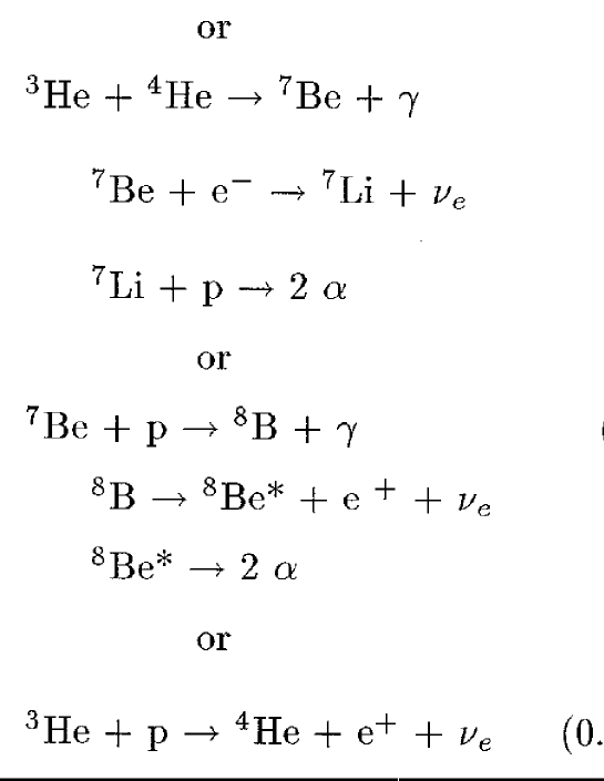
The pp, pep, ⁷Be and ⁸B neutrinos are produced in a set of nuclear reactions shown in Fig. 1. These make part of three major cycles (the pp-cycles) of nuclear fusion reactions in which effectively 4 protons burn into ⁴He with emission of two positrons and two neutrinos, generating approximately 98% of the solar energy:

$$4{\rm p}\rightarrow~{}^{4}{\rm He}+2{\rm e}^{+}+2\nu_{e}.~{}~{}$$

The first (pp-I) cycle (or chain) begins with the p-p (or p-e^--p) fusion into deuterium and ends with the reaction ${}^{3}{\rm He}+^{3}{\rm He}\rightarrow~{}^{4}{\rm He}+2p$. The second (pp-II) and the third (pp-III) cycles begin with the production of ⁷Be in ${}^{3}{\rm He}+^{4}{\rm He}$ fusion and end respectively with the processes ${}^{7}{\rm Li}+p\rightarrow~{}2^{4}{\rm He}$ and ${}^{8}{\rm B}\rightarrow~{}2^{4}{\rm He}+{\rm e}^{+}+\nu_{e}$ (see Fig. 1).

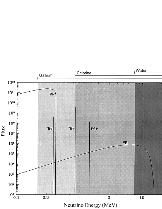
The CNO neutrinos are produced in the CNO-cycle of reactions, which, according to the present day understanding, plays minor role in the energetics of the Sun: ${}^{12}{\rm C}+p\rightarrow~{}^{13}{\rm N}+\gamma$, ${}^{13}{\rm N}\rightarrow~{}^{13}{\rm C}+{\rm e}^{+}+\nu_{e}$, ${}^{13}{\rm C}+p\rightarrow~{}^{14}{\rm N}+\gamma$, ${}^{14}{\rm N}+p\rightarrow~{}^{15}{\rm O}+\gamma$, ${}^{15}{\rm O}\rightarrow~{}^{15}{\rm N}+{\rm e}^{+}+\nu_{e}$ and ${}^{15}{\rm N}+p\rightarrow~{}^{12}{\rm C}+^{4}{\rm He}$. The pp, pep, ⁷Be and ⁸B neutrino spectra are depicted in Fig. 2. Let us note that the shapes of the continuous spectra of the pp, ⁸B and the CNO neutrinos are to a high degree of accuracy solar physics independent. The total fluxes of the pp, pep, ⁷Be, ⁸B and CNO neutrinos depend, although to a different degree, on the physical conditions in the central part of the Sun [JNB] (see further).

Figure 2: The spectra of the pp, pep, ⁷Be and ⁸B neutrino fluxes (from [23]). Shown are also the ranges of solar neutrino energies to which the Ga - Ge, Cl - Ar and Kamiokande II and III experiments are sensitive.

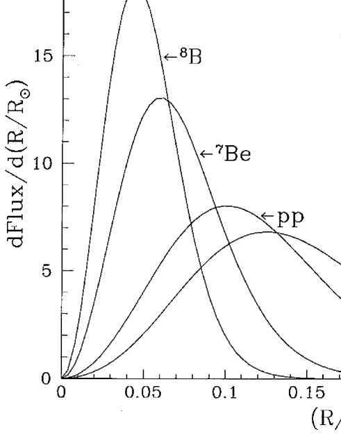
Solar neutrinos are produced in the central solar region (which practically coincides with energy production region) with radius $r_{\nu}\cong 0.25~{}R_{\odot}$, $R_{\odot}=6.96\times 10^{5}~{}{\rm km}$ being the radius of the Sun. The dependence of the source-strength functions for the pp, ⁷Be and ⁸B neutrinos on the distance from the center of the Sun, $r$, is shown in Fig. 3. As this figure illustrates, the major part of the ⁸B neutrinos flux is generated in a rather small region, $r\la 0.10~{}R_{\odot}$ close to the center of the Sun; the region of production of ⁷Be neutrinos extends to $r\cong 0.15~{}R_{\odot}$, while the region of the pp neutrino production is the largest extending to $r\cong 0.25~{}R_{\odot}$.

Figure 3: The production of the fluxes of pp, ⁷Be and ⁸B neutrinos as a function of the distance R from the center of the Sun (the latter is expressed in units of the solar radius ${\rm R_{\odot}}$) (from [23]).

Three different methods of solar neutrino detection have been and are being used in the six solar neutrino experiments [Davis], [Kam]–[SK] that have provided data so far: the Cl–Ar method proposed by Pontecorvo [Pont46] – in the experiment of Davis et al. [Davis68, Davis], the $\nu-e^{-}$ elastic scattering reaction – in the (Super-) Kamiokande experiments [Kam, SK], and the radiochemical Ga–Ge method – in SAGE [SAGE] and GALLEX [GALLEX] experiments.

The threshold energy of the reaction $\nu_{e}+^{37}{\rm Cl}\rightarrow e^{-}+^{37}{\rm Ar}$ on which the Cl–Ar method is based, is ${\rm E_{th}(Cl)=0.814~{}MeV}$. Consequently, the pp neutrinos do not give contributions in the signal in the Davis et al. detector. Inspecting the predictions of all solar models presently discussed in the literature one finds that the major contribution to the signal in the Cl–Ar experiment, between 64% and 79%, should be due to the ⁸B neutrinos; the ⁷Be neutrinos are predicted to generate between 22% and 13% of the total signal, and the pep and the CNO neutrinos – between 13% and 8%. With a threshold neutrino energy, E${}_{{\rm th}}({\rm K})$, first of 9.5 MeV (7.5 MeV) and subsequently reduced to 7.5 MeV and further to 7.3 MeV (6.5 MeV), the (Super-) Kamiokande experiments can detect only the higher energy ⁸B component of the solar $\nu_{e}$ flux.

Having the lowest threshold energy E${}_{{\rm th}}({\rm Ga})=~{}$0.233 MeV, the Ga–Ge detectors GALLEX and SAGE are sensitive to all six components of the flux considered above. Moreover, the major part of the signal in these detectors, between 51% and 63%, is predicted to be produced by the pp neutrinos; the ⁷Be neutrinos are expected to generate between 28% and 24% of the total signal, the ⁸B neutrinos – between 12% and 5%, and the CNO neutrinos – around (5–7)%.

The above analysis implies that the Cl–Ar and Kamiokande experiments on one side, and the Ga–Ge experiments on the other, are most sensitive to very different components of the solar neutrino flux: the former – to the ⁸B neutrinos, and the latter – to the pp neutrinos. The ⁷Be neutrinos are predicted to give the second largest (and non-negligible) contributions to the signals in both Cl–Ar and Ga–Ge experiments.

Let us turn next to the data. The average rate of ³⁷Ar production by solar neutrinos, $\bar{\rm R}$(Ar), observed in the experiment of Davis et al. in the period 1971–1996 (altogether $\sim 800$ solar $\nu_{e}$ induced events registered) is [Davis]

$$(2.56\pm 0.16\pm 0.14)\hskip 5.69046pt{\rm SNU}.$$ (1)

Here (and in the experimental results we quote further) the first error is statistical (1 s. d.) and the second error is systematic. The flux of ⁸B neutrinos, $\Phi_{{\rm B}}$, measured by the Kamiokande experiments reads [Kam]

$$\bar{\Phi}^{K}_{{\rm B}}=(2.80\pm 0.19\pm 0.33)\times 10^{6}~{}{\rm cm}^{-2}{\rm sec}^{-1}.$$ (2)

The result is based on a statistics of about 600 events accumulated by the two experiments in 2079 days of measurements in the period 1986 – 1996.

The GALLEX and SAGE experiments began to collect data in 1991 and 1990, respectively. The GALLEX group has registered (in 65 runs) approximately 300, and the SAGE group has registered (in 33 runs) about 100 solar neutrino induced events. The average rates of ⁷¹Ge production by solar neutrinos, $\bar{\rm R}({\rm Ge})$, measured by the two collaborations are [GALLEX, SAGE]

$$\bar{\rm R}_{\rm GALLEX}({\rm Ge})=(76.2~{}\pm 6.5~{}\pm 5)\hskip 5.69046pt{\rm SNU},$$ (3)

$$\bar{\rm R}_{{\rm SAGE}}({\rm Ge})=(73~{}\pm~{}8.5~{}^{+5.2}_{-6.9})\hskip 5.69046pt{\rm SNU}.$$ (4)

Obviously, the results of the two experiments are compatible. Adding the statistical and the systematical errors in (3) and in (4) in quadratures and combining the two results (i.e., taking the weighted average) we find

$$\bar{\rm R}_{{\rm exp}}({\rm Ge})=(75.4~{}\pm~{}7)\hskip 5.69046pt{\rm SNU}.$$ (5)

Recently, the Super-Kamiokande collaboration announced results on solar neutrinos based on data collected during a period of 306.3 days. About 4000 (!) solar neutrino induced events have been detected. The following value of the ⁸B neutrino flux was measured [SK]:

$$\bar{\Phi}^{SK}_{{\rm B}}=(2.44~{}\pm~{}0.06~{}^{+0.25}_{-0.09})\times 10^{6}~{}{\rm cm}^{-2}{\rm sec}^{-1}.$$ (6)

The GALLEX collaboration has successfully performed in 1994 and in 1997 very important (and rather spectacular) calibration experiments with an artificially prepared powerful ⁵¹Cr source of monoenergetic $\nu_{e}$ (four lines: E = 746 keV (81%), 751 keV (9%), 426 keV (9%) and 431 keV (1%)) of known intensity [GALLEX]. At the beginning of the two exposures the signal due to the ⁵¹Cr neutrinos was approximately 15 times bigger than the signal due to the solar neutrinos. The results of the experiments showed, in particular, that the efficiency of extraction of the ⁷¹Ge, produced by neutrinos, from the tank of the detector coincides (within the 10% error) with the calculated one.

Similar calibration experiment has been successfully completed in 1996 also by the SAGE collaboration. These experiments demonstrated, in particular, that the Ga-Ge detectors are capable of detecting the intermediate energy ⁷Be neutrinos with a high efficiency. They represent a solid proof that the data on the solar neutrinos provided by the two detectors are correct. They also represent the first real proof of the feasibility of the radiochemical method invented by Pontecorvo [Pont46] for detection and quantitative study of solar neutrinos.

An extensive program of calibration studies of the Super-Kamiokande detector is presently being completed. The aim is to reach an accuracy of 1% in the measurement of the energy of the recoil e^- from the solar neutrino induced reaction $\nu+e^{-}\rightarrow\nu+e^{-}$.

3 The Data Versus the Solar Model Predictions

3.1 Modeling the Sun

The results of the solar neutrino experiments have to be compared with the corresponding theoretical predictions. Many authors have worked (and many continue to work) in the field of solar modeling and have produced predictions for the values of the pp, ⁷Be, ⁸B, pep and CNO neutrino fluxes, and for the signals in the solar neutrino detectors: a rather detailed review of the results obtained by different authors prior 1992 and the corresponding references can be found in [BP92]. The articles [TCL], [Bert]–[DS96] describe some of the models proposed after 1992. Most persistently solar models with increasing sophistication and precision, aiming to account for and/or reproduce with sufficient accuracy the physical conditions and the possible processes taking place in the inner parts of the Sun have been developed starting from 1964 by John Bahcall and his collaborators [JNB].

The solar models are based on the standard assumptions of hydrostatic equilibrium and energy conservation made in the theory of stellar evolution. Several additional ingredients are needed to determine the physical structure of the Sun and its evolution in time [JNB, Cast2]:

1. the initial chemical composition,

2. the equation of state,

3. the rate of energy production per unit mass as a function of the density $\rho$, temperature T and chemical composition $\mu$,

4. the radiative opacity $\kappa$ as a function of the same three quantities, and

5. the mechanism of energy transport.

The initial chemical composition of the Sun is, of course, unknown. However, the relative abundances of the heavy elements in the initial Sun, with the exception of the noble gases and C, N, and O, are expected to be approximately equal to those found in the type I carbonaceous chondrite meteorites (see, e.g., [JNB]). Using the meteoritic abundances and the measured abundances in the solar photosphere which includes hydrogen, and taking into account the possible change of the heavy element abundances during the evolution of the Sun, permits to fix the present day ratio of the heavy element (Z) and hydrogen (X) mass fractions, Z/X. The knowledge of Z/X, the normalization condition $X+Y+Z=1$, where $Y$ is the helium mass fraction, and the requirement that the solar model reproduces correctly the measured value of the solar luminosity (see further) allows to determine the absolute values of the initial solar element abundances (for further details see [JNB]).

The equation of state requires the knowledge of the degree of ionization and the population of the excited states of all elements present in the Sun. Stellar plasma effects which introduce deviations from the perfect gas law have to be taken into account as well. As we have mentioned earlier, the energy is generated in the Sun in four cycles (or chains) of nuclear fusion reactions in which effectively 4 protons burn into ⁴He: $4{\rm p}\rightarrow~{}^{4}{\rm He}+2{\rm e}^{+}+2\nu_{e}$. Collective plasma and screening effects have to be accounted for in the calculation of the corresponding nuclear reaction cross-sections.

The radiative opacity $\kappa$ is determined by the photon mean free path. It controls the temperature gradient (and therefore the energy flow) in the radiative zone. The calculation of $\kappa$ requires a detailed knowledge of all atomic levels in the solar interior as well the cross-sections of photon scattering (elastic and inelastic), emission, absorption, inverse bremsstrahlung, etc. and is a rather complicated task. The energy transport is assumed to be by radiation in the inner part of the Sun, and by convection in the outer region. The border region between the radiative and convective zones is located at $r\sim 0.7R_{\odot}$, where $r$ is the distance from the solar center.

A solar model should reproduce the observed physical characteristics of the Sun: the mass [AstrAlmanac] $M_{\odot}=(1.98892\pm 0.00025)\times 10^{33}~{}{\rm g}$, the present radius $R_{\odot}=(6.9596\pm 0.0007)\times 10^{5}~{}{\rm km}$ and luminosity [BP95] (see also [PD]) $L_{\odot}=3.844(1\pm 0.004)\times 10^{33}~{}{\rm erg~{}s^{-1}}$, as well as the measured relative photospheric mass abundances of the elements heavier than ⁴He, Z, and of the hydrogen, X: $(Z/X)_{photo}=0.0245~{}(1\pm 0.061)$; actually, these quantities are used as input in the relevant computer calculations. An important constraint is the age of the Sun: $\tau_{\odot}=(4.57\pm 0.01)\times 10^{9}~{}{\rm yr}$. In order to develop a solar model one typically studies the evolution of an initially homogeneous Sun, having a mass $M_{\odot}$ during a period of time $\tau_{\odot}$. To reproduce the values of $R_{\odot}$, $L_{\odot}$ and $(Z/X)_{photo}$ at time $t=\tau_{\odot}$ three parameters in the calculations are used: the initial helium and heavy element abundances Y and Z, and a parameter characterizing the convection efficiency in the outer region of the Sun (the mixing length parameter). The latter is constrained by the value of $R_{\odot}$. It is usually assumed that the Sun is spherically symmetric.

It should be clear from the above brief discussion that the solar modeling requires a rather good knowledge of several branches of physics: astrophysics, atomic, nuclear (elementary particle) and plasma physics. The most recent and sophisticated standard solar models [Proff]–[DS96], [HELIOSEIS1] include the effects of the slow diffusion (relative to hydrogen) of helium and the heavier elements from the surface towards the center of the Sun (caused by the stronger gravitational pull of these elements relative to hydrogen).

3.2 Helioseismological Constraints on Solar Models

At present one of the most stringent constraints on the solar models are obtained from the helioseismological data. It was discovered experimentally as early as in 1960 [HELIOSEIS0] that the surface of the Sun is oscillating with periods which vary in the interval between about 15 and 3 minutes (these oscillations are usually referred to as the “5 minute oscillations”). In later studies about $10^{6}$ individual oscillation modes have been identified experimentally and their frequencies were measured with an accuracy of 1 part in $10^{4}$ or better.

The Sun’s surface oscillations reflect the existence of standing pressure waves (p-waves) in the interior of the Sun (see, e.g., [HELIOSEIS0]). Some of these waves penetrate deep into the region of neutrino production. The p-mode frequencies depend on the physical conditions in the interior of the Sun. Using a specially developed inversion technique and the more precise helioseismological data on the low-frequency oscillations which became available recently, it was possible to reconstruct with a remarkable accuracy the sound speed distribution, $c(r)$, in a large region of the Sun [HELIOSEIS0, HELIOSEIS1, HELIOSEIS2] extending from $r\cong 0.05~{}R_{\odot}$ to $r\cong 0.95~{}R_{\odot}$. Using the same data permitted to determine the location of the bottom of the convective zone, $r_{b}$, and the matter density at the bottom of the convective zone, $\rho_{b}$, as well [HELIOSEIS3]:

$$r_{b}=(0.708-0.714)~{}R_{\odot}~{},~{}~{}~{}$$

$$\rho_{b}=(0.185-0.199)~{}{\rm g/cm^{3}}~{}.~{}~{}~{}$$

The implications of the helioseismological data for the solar modeling are illustrated in Fig. 4 (taken from [HELIOSEIS2]), where the ratio $(c_{SM}(r)-c_{HS}(r))/c_{HS}(r)$, $c_{HS}(r)$ and $c_{SM}(r)$ being the sound speed distributions extracted from the helioseismological data and predicted by a given solar model, is plotted for two solar models - without and including heavy element diffusion [BP95]. Only the statistical errors in the determination of $c_{HS}(r)$ are shown (they are so small that they are barely seen), but the general conclusions which can be inferred from such a comparison remain valid after the inclusion of conservatively estimated systematical errors [HELIOSEIS3]. As Fig. 4 illustrates, the difference between $c_{HS}(r)$ and $c_{SM}(r)$ for the model without heavy element diffusion is so large that this model is practically ruled out by the helioseismological data. Actually, the same conclusion is valid for all existing solar models without heavy element diffusion (e.g., the models [BP92, TCL, Cast1]).

Further studies [HELIOSEIS3] have shown, in particular, that models which have been especially designed to explain the observed deficiency of ⁸B neutrinos by lowering the temperature in the central region of the Sun (see further), i.e., the so-called models with “mixed solar core”, also do not pass the helioseismological data test. Thus, of the large number of solar models proposed so far only the models which include diffusion of the heavy elements are compatible with the helioseismological data.

Figure 4: The ratio $(c_{SM}-c_{HS})/c_{HS}$, $c_{HS}$ and $c_{SM}$ being the sound speed distributions extracted from the helioseismological data and predicted by a given solar model, as a function of the distance $R$ from the center of the Sun (expressed in units of the solar radius ${\rm R_{\odot}}$) (from [36]). The ratio is plotted for two solar models – without (dashed line) and including (solid line) heavy element diffusion [29]. Only the statistical errors in the determination of $c_{HS}(r)$ are included in the analysis (they are too small to be seen).

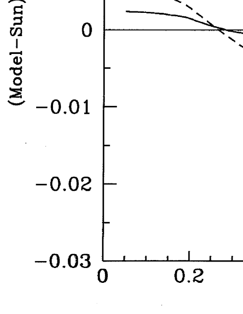
The agreement of the predictions of the models with heavy element diffusion for $c(r)$ with the sound speed distribution deduced from the data is quite impressive. As Fig. 4 indicates, the root mean square (r.m.s.) deviation from $c_{HS}(r)$ for the model of [BP95] in the entire range of $c_{HS}(r)$ determination is $\sim 0.1\%$. For the model with heavy element diffusion of [HELIOSEIS1] the r.m.s. discrepancy is $\sim 0.2\%$. Adding the estimated systematic uncertainties in the determination of $c_{HS}(r)$ allows the difference $|c_{SM}(r)-c_{HS}(r)|$ to be somewhat larger [HELIOSEIS3] : the ratio $|c_{SM}(r)-c_{HS}(r)|/c_{HS}(r)$ for the model [BP95], however, does not exceed approximately 0.4% in the region $0.2R_{\odot}\leq r\leq 0.65R_{\odot}$, and about 1% in the neutrino production region $0.05R_{\odot}\leq r\leq 0.20R_{\odot}$, for which the helioseismological data is less accurate.

As can be shown [HELIOSEIS2], in the interior of the Sun one has: $c^{2}(r)\sim T(r)/\mu(r)$, where $T$ is the temperature and $\mu$ is the mean molecular weight. Consequently, even small deviations of the solar model predictions for $T$ and $\mu$ from their actual values in the Sun, $\delta T$ and $\delta\mu$, would lead to a relatively large discrepancy between the predicted an measured values of $c(r)$: $\delta c/c\cong 0.5(\delta T/T-\delta\mu/\mu)$. Since, according by the standard solar models, $T$ and $\mu$ vary by very different factors in the energy (neutrino) production region, namely, by a factor of 1.9 and by 39%, it is quite unlikely that the discrepancies between the predicted and actual values of $T$ and $\mu$ mutually cancel to produce the remarkable agreement for the models with heavy element diffusion, illustrated in Fig. 4. Barring such a cancellation, the comparison between $c_{HS}(r)$ and $c_{SM}(r)$ suggests that for the indicated models $|\delta T|/T$, $|\delta\mu|/\mu\la 2\%$ in the interior of the Sun, and is considerably smaller in most part of the Sun. Since the solar neutrino fluxes scale approximately as $T_{c}^{n}$ with $n=-1.1;~{}8;~{}24$ respectively for the pp, ⁷Be and ⁸B neutrinos [BUlmer96], $T_{c}$ being the central temperature predicted by the model, the above results implies, in particular, that it is impossible to reduce considerably even the ⁸B neutrino flux by changing the central temperature within the limits following from the helioseismological data.

3.3 Predictions for the Neutrino Fluxes and the Signals in the Solar Neutrino Detectors

We shall present here the results obtained in four models [BP95]–[DS96] with heavy element diffusion, which can be characterized by their predictions for the total flux of ⁸B neutrinos as relatively “high flux” [BP95, RVCD], “intermediate flux” [Cast2] and “low flux” [DS96] models. The predictions for the ⁸B neutrino flux and for the signals in the solar neutrino detectors in these models determine the corresponding intervals in which the results of practically all contemporary solar models compatible with the helioseismological data [HELIOSEIS01]–[HELIOSEIS3] lie (see, e.g., [Proff, HELIOSEIS1]). Thus, they give an idea about the dispersion and the possible uncertainties in the predictions.

In Table 1 we have collected the results of the models of Bahcall–Pinsonneault (BP’95) from 1995 [BP95], Richard et al. (RVCD) [RVCD], Castellani et al. (CDFLR) [Cast2], and of Dar and Shaviv from 1996 (DS’96) [DS96] for the values of the fluxes of the pp, ⁷Be, ⁸B, pep and CNO neutrinos at the Earth surface. We have included also the estimated 1 s.d. uncertainties in the predictions for the fluxes made by Bahcall and Pinsonneault for their model. In Tables 2 and 3 we give the predictions for the contributions of each of the indicated six fluxes to the signals in the Cl–Ar [Davis] and the Ga–Ge [SAGE, GALLEX] experiments, respectively, and quote the predictions for the total signals in these experiments (including the estimated 1 s.d. uncertainty in the predictions whenever it is given by the authors).

A comparison between the experimental results (1) – (6) and the corresponding predictions given in Tables 2 and 3 leads to the conclusion that none of the solar models proposed so far provides a satisfactory description of the solar neutrino data: the predictions typically exceed the observations. This is one of the current aspects of the solar neutrino problem.

Table 1: Solar neutrino fluxes at the Earth surface (in units of cm^-2sec^-1) predicted by the solar models [29]–[32].

Flux of neutrinos	BP’95	RVCD	CDFLR	DS’96
$\Phi_{\rm pp}\times 10^{-10}$	$5.91(1~{}^{+0.01}_{-0.02})$	$5.94$	$5.99$	$6.10$
$\Phi_{\rm pep}\times 10^{-8}$	$1.40(1~{}^{+0.01}_{-0.02})$	$1.38$	$1.40$	$1.43$
$\Phi_{\rm Be}\times 10^{-9}$	$5.15(1~{}^{+0.06}_{-0.07})$	$4.80$	$4.49$	$3.71$
$\Phi_{\rm B}\times 10^{-6}$	$6.62(1~{}^{+0.14}_{-0.17})$	$6.33$	$5.16$	$2.49$
$\Phi_{\rm N}\times 10^{-8}$	$6.18(1~{}^{+0.17}_{-0.20})$	$5.59$	$5.30$	$3.82$
$\Phi_{\rm O}\times 10^{-8}$	$5.45(1~{}^{+0.19}_{-0.22})$	$4.81$	$4.50$	$3.74$

Table 2: Signals (in SNU) in Cl–Ar detectors due to the solar neutrinos, predicted by the solar models [29]–[32].

Type of neutrinos	BP’95	RVCD	CDFLR	DS’96
pp	$0.0$	$0.0$	$0.0$	$0.0$
pep	$0.22$	$0.22$	$0.22$	$0.24$
7Be	$1.24$	$1.15$	$1.08$	$0.89$
8B	$7.36$	$6.71$	$5.74$	$2.64$
13N	$0.11$	$0.09$	$0.09$	$0.06$
15O	$0.37$	$0.32$	$0.31$	$0.25$
Total:	$9.3~{}^{+1.2}_{-1.4}$	$8.5$	$7.4$	$4.1~{}\pm~{}1.2$

Taking into account the estimated uncertainties in the theoretical predictions and the experimental errors in (1) – (6) one finds that the differences between the predictions and the observations are largest for the “high flux” models: the measured values of $\bar{\rm R}$(Ar), $\bar{\Phi}$(B) and $\bar{\rm R}({\rm Ge})$ in the Cl–Ar, Kamiokande and Ga–Ge experiments are at least by (3.5–4.0) s.d. smaller than the predicted ones in [BP95, RVCD]. The “low flux” model of Dar and Shaviv reproduces the result of the Kamiokande and Super-Kamiokande experiments for $\bar{\Phi}$(B). However, the prediction of the model for $\bar{\rm R}({\rm Ge})$ is respectively by at least 3 s.d. higher than the GALLEX and SAGE results (3) and (4). The discrepancy between the solar model predictions and the Ga–Ge data is somewhat larger if one compares the predictions with the combined result (5) of the GALLEX and SAGE experiments.

Table 3: Signals (in SNU) in Ga–Ge detectors due to the solar neutrinos, predicted by the solar models [29]–[32].

Type of neutrinos	BP’95	RVCD	CDFLR	DS’96
pp	$69.7$	$70.1$	$70.7$	$72.0$
pep	$3.0$	$3.0$	$3.0$	$3.0$
7Be	$37.7$	$35.3$	$32.9$	$27.1$
8B	$16.1$	$15.4$	$12.6$	$6.1$
13N	$3.8$	$3.5$	$3.3$	$2.4$
15O	$6.3$	$5.6$	$5.2$	$4.6$
Total:	$137~{}^{+8}_{-7}$	$133$	$128$	$115~{}\pm~{}6.0$

Let us discuss in somewhat greater detail the results of the four representative models [BP95]–[DS96] for the fluxes of the pp, pep, ⁷Be, ⁸B and CNO neutrinos shown in Table 1. The predictions for the values of the pp and pep neutrino fluxes are remarkably coherent: they very from model to model at most by 3% and 3.5%, respectively. Actually, the two fluxes are related [JNB]: $\Phi_{\rm pep}$ is proportional to $\Phi_{\rm pp}$ and the coefficient of proportionality is practically solar model independent, being determined by the ratio of the cross–sections of the reactions ${\rm p+e^{-}+p\rightarrow D+\nu_{e}}$ and ${\rm p+p\rightarrow D+e^{+}+\nu_{e}}$ in which the pep and pp neutrinos are produced in the Sun. One has [JNB]–[DS96]

$$\Phi_{\rm pep}=(2.3-2.4)\times 10^{-3}\Phi_{\rm pp}.~{}~{}~{}$$

The value of the pp flux is constrained by the existing rather precise data on the solar luminosity, L_⊙. Indeed [Lumin], the solar luminosity is determined by the thermal energy released in the Sun in the two well known cycles of nuclear reactions, the pp (Fig. 1) and the CNO cycles (see, e.g., [JNB]), in which 4 protons are converted into ⁴He with emission of 2 neutrinos. From the point of view of the energy effectively generated, the indicated hydrogen burning reactions can be written as

$$4{\rm p}+2{\rm e}^{-}\rightarrow~{}^{4}{\rm He}+2\nu_{e}.~{}~{}$$

Depending on the cycle, the two emitted neutrinos can be both of the pp or pep type, or a pp (pep) and a ⁷Be, a pp (pep) and a ⁸B (pp cycle), and a ¹⁵O and/or ¹³N (CNO cycle) neutrinos [JNB, Cast2]. The thermal energy released per one produced pp, pep, ⁷Be and ⁸B neutrino is equal to $({\rm Q}/2-\bar{\rm E}_{{\rm j}})$, where Q $=$ 26.732 MeV is the Q–value of the reaction (7), and $\bar{\rm E}_{{\rm j}}$ is the average energy of the neutrino of the type j (j = pp, …). The energy released per one ¹⁵O and/or one ¹³N neutrino, as can be shown (taking into account, in particular, the discussion of the rates of the different reactions of the CNO cycle given in [JNB]) is equal with a high precision to the difference $({\rm Q}/2-(\bar{\rm E}_{{\rm N}}+\bar{\rm E}_{{\rm O}})/2)$. Obviously, the values of Q and $\bar{\rm E}_{{\rm j}}$ are solar physics (and therefore solar model) independent.

Given the average energies $\bar{\rm E}_{{\rm j}}$ carried away by the pp, pep, ⁷Be, ⁸B and CNO neutrinos (they are listed at the beginning of Sect. 2, $\bar{\rm E}_{{\rm Be}}=0.813~{}$MeV), and knowing that the energy emission by the Sun is quasi-stationary (steady state), it is possible to relate L_⊙ with the pp, pep, ⁷Be, ⁸B and CNO neutrino luminosities of the Sun. One finds in this way the following constraint on the solar neutrino fluxes:

$$\Phi_{\rm pp}+0.958\,\Phi_{\rm Be}+0.955\,\Phi_{\rm CNO}+0.910\,\Phi_{\rm pep}=(6.514~{}\pm~{}0.031)\times 10^{10}~{}{\rm cm}^{-2}{\rm sec}^{-1}~{},~{}~{}$$

where

$$\Phi_{\rm CNO}=\Phi_{\rm N}+\Phi_{\rm O}\,,$$

we have used [BP95] (see also [AstrAlmanac, PD]) L${}_{\odot}=(3.844~{}\pm~{}0.015)\times 10^{33}~{}{\rm erg}~{}{\rm sec}^{-1}$ and have neglected the terms proportional to $\Phi_{\rm B}$ and to $(\Phi_{\rm N}-\Phi_{\rm O})$ in the left hand side of the equation, which are predicted to be considerably smaller than $3\times 10^{8}~{}{\rm cm}^{-2}{\rm sec}^{-1}$. The fluxes $\Phi_{\rm B}$ and $(\Phi_{\rm N}-\Phi_{\rm O})$ have to be more than 46 and (3 - 4) times bigger than the largest (“high flux”) model predictions [BP95] and [RVCD], respectively, in order for these terms to exceed the indicated value. The coefficient multiplying the $\Phi_{\rm Be}$ term in (11) is just the ratio of the thermal energies produced per one ⁷Be and one pp neutrino, $({\rm Q}/2-\bar{\rm E}_{{\rm Be}})$/$({\rm Q}/2-\bar{\rm E}_{{\rm pp}})$, etc. Since, as Table 1 shows, $\Phi_{\rm Be}$ and $\Phi_{\rm CNO}$ are smaller than $\Phi_{\rm pp}$ at least by the factors 0.09 and 0.02, respectively, and $\Phi_{\rm pep}$ is even smaller (see (9)), (11) limits primarily the pp neutrino flux.

Comparing the experimental results (3) – (6) with the solar model predictions given in Table 3 one notices, in particular, that the rate of ⁷¹Ge production due only to the pp neutrinos, R${}^{{\rm pp}}({\rm Ge})=(70-72)~{}$SNU, is very close to the rates observed in the GALLEX and SAGE experiments. This suggests that a large fraction, i.e., roughly at least half, of the pp (electron) neutrinos emitted by the Sun reach the Earth intact and are detected.

The relative spread in the predictions for the ⁷Be neutrino flux $\Phi_{\rm Be}$ and for the signals due to the ⁷Be neutrinos in the Cl–Ar and Ga–Ge experiments, as it follows from Tables 1 – 3, does not exceed approximately 30%.

4 The ⁸B Neutrino Problem

A further inspection of the results collected in Table 1 reveals that the differences (and the estimated uncertainties) in the predictions of the solar models for the total flux of ⁸B neutrinos are the largest: the value of $\Phi_{\rm B}$ in the models [BP95]–[Cast2] is by more than a factor of 2 larger than the value obtained in the “low flux” model [DS96]. The ⁸B neutrinos are born in the Sun in the $\beta^{+}$-decay, ${}^{8}{\rm B}\rightarrow~{}^{8}{\rm Be}^{*}+{\rm e}^{+}+\nu_{e}$, of the ⁸B nucleus which is produced in the reaction

$${\rm p}+~{}^{7}{\rm Be}\rightarrow~{}^{8}{\rm B}+\gamma~{}~{}~{}$$

initiated by $\sim$20 keV protons. Obviously, $\Phi_{\rm B}$ is proportional to the rate of the process (12) taking place in the solar plasma environment, which in turn is to large extent determined by the cross–section of (12), $\sigma_{{\rm 17}}({\rm E_{p}})$. The latter is usually represented in the form [JNB]

$$\sigma_{{\rm 17}}({\rm E_{p}})={{\rm S_{17}(E_{p})}\over{{\rm E_{p}}}}~{}{\rm exp(-8\pi~{}e^{2}/v)},~{}~{}~{}$$

where ${\rm exp(-8\pi~{}e^{2}/v)}$ is the Gamow penetration factor, and E_p and v are the p – ⁷Be c.m. kinetic energy and relative velocity. The largely different values of the astrophysical factor ${\rm S_{17}}$, ${\rm S_{17}}\equiv{{\rm S_{17}({\rm E_{p}\sim 20~{}keV})}}$, adopted by the authors of [BP95, RVCD, Cast2] and of [DS96] is one of the major sources of the large spread in the predictions for $\Phi_{\rm B}$.

Because of background problems it is impossible to measure the cross–section $\sigma_{{\rm 17}}({\rm E_{p}})$ directly at the low energies of the incident protons, which are of astrophysical interest. The experimental studies of the process (12) were performed at energies $110~{}{\rm keV}\leq{\rm E_{p}}\la 2000~{}$keV. They are technically rather difficult because of the instability of the ⁷Be serving as a target. The results obtained in the indicated higher energy domain are extrapolated to ${\rm E_{p}}\sim 20~{}$keV using a theoretical model describing the data (and the process (12) in the entire energy range $20~{}{\rm keV}\leq{\rm E_{p}}\la 2000~{}$keV) and taking into account the possible solar plasma screening effects. Obviously, there are at least two major sources of uncertainties in the determination of ${\rm S_{17}}$ inherent to the indicated approach: the uncertainties associated with the data at ${\rm E_{p}}\geq 110~{}$keV, and those associated with the extrapolation procedure exploited.

Altogether six experiments have provided data on the the p – ⁷Be cross–section $\sigma_{{\rm 17}}({\rm E_{p}})~{}$ so far. The results of the four most accurate of them [Kavanagh, Filip] can be grouped in two distinct pairs, [Kavanagh] and [Filip], which agree on the energy dependence of ${\rm S_{17}(E_{p})}$, but disagree systematically by $~{}\sim$ (20–25)% ($~{}\sim$(2–3) s.d.) on the absolute values of ${\rm S_{17}(E_{p})}$. The authors of [BP95, Cast2] (and, we suppose, of [RVCD]) used in their calculations the value ${\rm S_{17}}=(22.4~{}\pm~{}2.1)~{}$eV-b derived by extrapolation in [John] on the basis of the data from all six experiments.

A new method of experimental determination of ${\rm S_{17}}$ was proposed relatively recently in [Moto]. It is based on the idea of measuring the cross-section of the inverse reaction, $\gamma+~{}^{8}$B $\rightarrow~{}^{7}$Be$~{}+~{}$p, by studying the dissociation of ⁸B into p + ⁷Be in the Coulomb field of a heavy nucleus, chosen to be ²⁰⁸Pb. The time–reversal symmetry guarantees that the cross–sections of (12) and of the inverse reaction should be equal. The extraction of the values of $\sigma_{{\rm 17}}({\rm E_{p}})$ (and of ${\rm S_{17}(E_{p})}$) from the data on the process ${}^{8}{\rm B+~{}^{208}Pb}\rightarrow{\rm p}+~{}^{7}{\rm Be+~{}^{208}Pb}$ is not straightforward and is associated with certain subtleties (see, e.g., [Lang]).

Using the results of the experiment of Motobayashi et al. [Moto] on the reaction ${}^{8}{\rm B+~{}^{208}Pb}\rightarrow{\rm p}~{}+~{}^{7}{\rm Be+~{}^{208}Pb}$ to determine the cross-section $\sigma_{{\rm 17}}({\rm E_{p}})$ in the energy interval $500~{}{\rm keV}\la{\rm E_{p}}\la 2000~{}$keV, the results of the most recent of the experiments on (12) of Filippone et al. [Filip] in the interval (110 – 500) keV, and a new extrapolation model developed by them, the authors of [DS96] obtain ${\rm S_{17}}=17\pm 2~{}$eV-b. 

The additional difference between the values of $\Phi_{\rm B}$ predicted in [BP95] and in [DS96] is due to

1. the use of different (but still compatible within the errors with the measured or deduced from the data) values of other relevant nuclear reaction cross–sections, as those of the ${}^{3}{\rm He+~{}^{3}He}\rightarrow~{}^{4}{\rm He+2p}$ and ${}^{3}{\rm He+~{}^{4}He}\rightarrow~{}^{7}{\rm Be}+\gamma~{}$ reactions (a factor $\sim 1.2$), and

2. the use in [BP95] and in [DS96] of different methods to account for the diffusion of the heavy elements in the Sun.

The latter leads, in particular, to a difference in the values of the central temperature in the Sun in the models [BP95] and [DS96]: ${\rm T_{c}(BP^{\prime}95)=1.584\times 10^{7}~{}K}$ and ${\rm T_{c}(DS^{\prime}96)=1.561\times 10^{7}~{}K}$. As the ⁸B neutrino flux $\Phi_{\rm B}$ is very sensitive to the value of T_c, scaling as [BUlmer96] $\Phi_{\rm B}\sim{\rm T}^{24}_{\rm c}~{}$, the indicated difference in T_c implies an additional difference in the values of $\Phi_{\rm B}$ predicted in [BP95] and in [DS96] (a factor of $\sim 1.4$).

5 The Missing ⁷Be Neutrinos

Even if one accepts that there are large uncertainties in the predictions for the flux of ⁸B neutrinos and in all analyses one should rather use for $\Phi_{\rm B}$ the value implied by the (Super-) Kamiokande data, (2) and (6), another problem arises: the predictions of all contemporary solar models for the flux of ⁷Be neutrinos, $\Phi_{\rm Be}$, are considerably larger than the value suggested by the existing solar neutrino data. This was first noticed in [BachBe] and confirmed in several subsequent more detailed studies [Cast3]–[Bach2] utilizing a variety of different methods. We shall illustrate here the above result using rather simple arguments [BachBe, Bach2].

Let us assume that the spectrum of the ⁸B neutrino flux coincides with that predicted by the solar models, i.e., with the spectrum of the $\nu_{e}$ emitted in the decay ${}^{8}{\rm B}\rightarrow~{}^{8}{\rm Be}^{*}+{\rm e}^{+}+\nu_{e}$ (see Fig. 2). This would be the case if the solar ⁸B $\nu_{e}$ behave conventionally during their journey to the Earth. For the value of the total ⁸B neutrino flux one can use the Super-Kamiokande result (6): $\bar{\Phi}^{SK}_{{\rm B}}=(2.44~{}^{+0.26}_{-0.11})\times 10^{6}~{}{\rm cm}^{-2}{\rm sec}^{-1}$, where the statistical and the systematic errors were added in quadratures. Knowing ${\rm\Phi_{B}}$ and the the cross-section [JNB] of the Pontecorvo–Davis reaction $\nu_{e}+^{37}{\rm Cl}\rightarrow e^{-}+^{37}{\rm Ar}$, one can calculate the contribution of the ⁸B neutrinos to the signal in the Davis et al. experiment, ${\rm R^{B}(Ar)}$. One finds:

$${\rm R^{B}(Ar)}=(2.71~{}^{+0.30}_{-0.14})~{}{\rm SNU}.~{}~{}$$

By subtracting this value from the rate of Ar production measured in the Davis et al. experiment we obtain the sum of the contributions of the ⁷Be, pep and CNO neutrinos to the signal in this experiment:

$${\rm R^{Be+pep+CNO}(Ar)}=~{}(-0.15~{}^{+0.37}_{-0.25})~{}{\rm SNU}.~{}~{}~{}$$

Given the solar model independent relation (9) between ${\rm\Phi_{pep}}$ and ${\rm\Phi_{pp}}$, and that ${\rm\Phi_{pp}}$ is rather tightly constrained by the data on the solar luminosity, we can consider as rather reliable (and weakly model dependent) the solar model predictions for ${\rm R^{pep}_{SM}(Ar)}=(0.22-0.24)~{}$SNU. Taking ${\rm R^{pep}(Ar)}=0.22~{}$SNU one obtains from (15)

$${\rm R^{Be}(Ar)}\leq~{}(-0.37~{}^{+0.37}_{-0.25})~{}{\rm SNU},~{}~{}~{}$$

${\rm R^{Be}(Ar)}$ being the ⁷Be neutrino contribution to the signal in the Davis et al. experiment. At 99.73% C.L. (3 s.d.) this implies ${\rm R^{Be}(Ar)}\leq 0.74~{}{\rm SNU}$, which is smaller than the predictions of the solar models with heavy element diffusion, ${\rm R^{Be}_{SM}(Ar)}=(0.89-1.24)~{}{\rm SNU}~{}$ [Proff, BP95, RVCD, Cast2, DS96, HELIOSEIS1]. As ${\rm R^{Be}(Ar)}\sim\Phi_{\rm Be}$, the result obtained suggests that, if the solar neutrinos are assumed to behave conventionally on the way to the Earth (i.e., do not undergo oscillations, transitions, decays, etc.), the ⁷Be $\nu_{e}$ flux inferred from the solar neutrino data is substantially smaller than the flux predicted by the contemporary solar models.

Similar (though statistically somewhat weaker) conclusions can be reached for the contribution of the ⁷Be neutrinos to the signal in the Ga-Ge detectors, ${\rm R^{Be}(Ge)}$, and correspondingly for $\Phi_{\rm Be}$, by taking into account the fact that the solar model predictions for the contributions of the pp and pep neutrinos to the indicated signal, ${\rm R^{pp+pep}(Ge)}$, are tightly constrained by the data on the solar luminosity and vary by no more than 3%: ${\rm R^{pp+pep}_{SM}(Ge)}=(72.7-75.0)~{}{\rm SNU}$. Subtracting ${\rm R^{pp+pep}_{SM}(Ge)}=72~{}{\rm SNU}$ from the rate of Ge production observed in the SAGE and GALLEX experiments, Eq. (5), one obtains for the contribution of ⁸B, ⁷Be and CNO neutrinos: ${\rm R^{B+Be+CNO}(Ge)}=(3.4~{}\pm~{}7)~{}{\rm SNU}$.

Utilizing the value of $\bar{\Phi}^{SK}_{{\rm B}}$ measured by the Super-Kamiokande experiment and the Ga–Ge reaction cross–section [JNB, Bach2] permits to calculate the contribution of the ⁸B neutrinos, ${\rm R^{B}(Ge)}$, to ${\rm\bar{R}_{exp}(Ge)}$: ${\rm R^{B}(Ge)}=(5.9~{}^{+5.9}_{-2.9})~{}{\rm SNU}$, where the error is dominated by the estimated uncertainty in the value of the Ga–Ge reaction cross–section [Bach2]. Subtracting the so derived value of ${\rm R^{B}(Ge)}$ from the value of ${\rm R^{B+Be+CNO}(Ge)}$ we get:

$${\rm R^{Be}(Ge)}\leq~{}(-2.5~{}^{+9.2}_{-7.6})~{}{\rm SNU}.~{}~{}~{}$$

Consequently, at 99.73% C.L. (3 s.d.) the contribution of ⁷Be neutrinos to the signals in the SAGE and GALLEX experiments does not exceed 25.1 SNU, while the solar models [BP92]–[DS96], [HELIOSEIS2] predict ${\rm R^{Be}(Ge)}\geq 27~{}{\rm SNU}$.

Analogous results have been obtained in [Cast3, KwRos] using different methods. The same conclusion has been reached in [HatLang1] as well on the basis of a $\chi^{2}-~{}$analysis of the solar model description of the data, in which the total pp, pep, ⁷Be, ⁸B and CNO neutrino fluxes were treated as free parameters subject only to the luminosity constraint (11), while the spectra of solar neutrinos were assumed to coincide with the predicted ones in the absence of unconventional neutrino behaviour (as oscillations in vacuum, etc.).

Thus, there are strong indications from the existing solar neutrino data that the flux of ⁷Be (electron) neutrinos is considerably smaller than the flux predicted in all contemporary solar models. Given the results of the GALLEX and SAGE calibration experiments, we can conclude that both the Davis et al. and the Super-Kamiokande (Kamiokande) data, (2) and (6) (Eq. (3)), have to be incorrect in order for the above conclusion to be not valid. The discrepancy between the value of $\Phi_{{\rm Be}}$ suggested by the analyses of the existing solar neutrino data and the solar model predictions for $\Phi_{{\rm Be}}$ represents the major new aspect of the solar neutrino problem. No plausible astrophysical and/or nuclear physics explanation of this discrepancy has been proposed so far.

6 Neutrino Physics Solutions of the Solar Neutrino Problem

We have seen that none of the solar models developed during the last ten years provides a satisfactory description of the existing solar neutrino data. The discrepancy between the data and the solar model predictions is especially large for the majority of models with heavy element diffusion, which are compatible with the helioseismological data. The solar model predictions for the signals caused by the solar neutrinos in the solar neutrino experiments are larger than the measured signals. In particular, no solar, atomic or nuclear physics solution to the ⁷Be neutrino problem discussed above was found so far. Since the solar neutrino detectors are sensitive either only, or predominantly, to the solar $\nu_{e}$ flux, these results indicate that the solar $\nu_{e}$ flux is depleted on the way to the Earth.

Such a depletion can take place naturally if the solar $\nu_{e}$ undergo transitions into neutrinos of a different type, $\nu_{\mu}$ and/or $\nu_{\tau}$, and/or into a sterile neutrino $\nu_{s}$, or are converted into antineutrinos $\bar{\nu}_{\mu}$ and/or $\bar{\nu}_{\tau}$, while they travel to the Earth. The depletion of the solar $\nu_{e}$ flux might be caused also by instability of the solar neutrinos which can decay on their way to the Earth. Thus, several physically rather different neutrino physics solutions of the solar neutrino problem are, in principle, possible. They all require the existence of “unconventional” intrinsic neutrino properties (mass, mixing, magnetic moment) and/or couplings (e.g., flavour changing neutral current (FCNC) interactions). More specifically, these solutions include:

1. oscillations in vacuum [Pont57, Pont67, NMP2] of the solar $\nu_{e}$ into different weak eigenstate neutrinos ($\nu_{\mu}$ and/or $\nu_{\tau}$, and/or sterile neutrinos, $\nu_{s}$) on the way from the surface of the Sun to the Earth [KP1]–[BerRos],

2. matter-enhanced transitions [MSW1, MSW2] $\nu_{e}\rightarrow\nu_{\mu(\tau)}$, and/or $\nu_{e}\rightarrow\nu_{s}$, while the solar neutrinos propagate from the central part to the surface of the Sun [KP4]–[KP5],

3. solar $\nu_{e}$ resonant spin or spin-flavour conversion (RSFC) in the magnetic field of the Sun [RSFP1], and

4. matter-enhanced transitions, for instance $\nu_{e}\rightarrow\nu_{\tau}$, in the Sun, induced by flavour changing neutral current (FCNC) interactions of the solar $\nu_{e}$ with the particles forming the solar matter [FCNC1]–[FCNC3] (these transitions can take place even in the case of absence of lepton mixing in vacuum and massless neutrinos [FCNC1]).

All these possibilities have been and continue to be extensively studied (see the quoted articles). There have not been recent studies of the solar neutrino decay hypothesis [DEC1] which, however, was disfavored [DEC2] by the earlier solar neutrino data.

In what follows we shall discuss the vacuum oscillation and the matter-enhanced transition solutions of the solar neutrino problem. The status of these solutions has been reviewed recently, e.g., in [SPnu96, SPHeid97].

6.1 Oscillations in Vacuum

Neutrino oscillations in vacuum [Pont57], have been discussed in connection with the solar neutrino experiments [Pont67] and as a possible solution of the solar neutrino problem [NMP2, NMP1], [KP1]–[BerRos], [SPHeid97] (and the literature quoted therein) for about 31 years. In the simplest version of this scenario it is assumed that the state vector of the electron neutrino, $|\nu_{e}\rangle$, produced in vacuum with momentum $p$ in some weak interaction process, is a coherent superposition of the state vectors $|\nu_{i}\rangle$ of two neutrinos $\nu_{i}$, i=1,2, having the same momentum $p$ and definite but different masses in vacuum, ${\rm m_{i}}$, ${\rm m_{1}}\neq{\rm m_{2}}$, while the linear combination of $|\nu_{1}\rangle$ and $|\nu_{2}\rangle$, which is orthogonal to $|\nu_{e}\rangle$, represents the state vector $|\nu_{x}\rangle$ of another weak-eigenstate neutrino, $|\nu_{x}\rangle~{}=|\nu_{\mu(\tau)}\rangle$ or $|\nu_{s}\rangle$:

$$|\nu_{e}\rangle~{}=|\nu_{1}\rangle\cos\theta+|\nu_{2}\rangle\sin\theta~{},~{}~{}~{}~{}$$

$$|\nu_{x}\rangle~{}=-|\nu_{1}\rangle\sin\theta+|\nu_{2}\rangle\cos\theta~{},~{}~{}~{}$$

where $\theta$ is the neutrino (lepton) mixing angle in vacuum. We shall assume for concreteness in what follows that $\nu_{x}$ is an active neutrino, say $\nu_{\mu}$, $|\nu_{x}\rangle~{}=|\nu_{\mu}\rangle$.

Obviously, the states $|\nu_{1,2}\rangle$ are eigenstates of the Hamiltonian of the neutrino system in vacuum, $H_{0}$:

$$H_{0}~{}|\nu_{i}\rangle~{}=E_{i}~{}|\nu_{i}\rangle,~{}~{}~{}E_{i}=\sqrt{\mbox{\boldmath{$p$}}^{2}+m_{i}^{2}},~{}i=1,2.~{}~{}~{}$$

If $\nu_{e}$ is produced at time $t=0$ in the Sun in the state given by (18a), after a time $t$ the latter will evolve into the state

$$|\nu_{e}(t)\rangle~{}=e^{-iE_{1}t}~{}|\nu_{1}\rangle\cos\theta+e^{-iE_{2}t}~{}|\nu_{2}\rangle\sin\theta~{},$$

where we have ignored the overall space coordinate dependent factor ${\rm exp}(i\,\mbox{\boldmath{$p$}}\,\mbox{\boldmath{$r$}})$ in the right-hand side of (20) and have assumed that the solar matter does not affect the evolution of the neutrino system. (The possible effects of matter on the evolution of the neutrino state will be considered in the next Section.) Using (18a) and (18b) to express the vectors $|\nu_{1}\rangle$ and $|\nu_{2}\rangle$ in terms of the vectors $|\nu_{e}\rangle$ and $|\nu_{\mu}\rangle$ we can rewrite (20) in the form:

$$|\nu_{e}(t)\rangle~{}=A_{ee}(t)~{}|\nu_{e}\rangle+A_{\mu e}(t)~{}|\nu_{\mu}\rangle~{},~{}~{}~{}$$

where

$$A_{ee}(t)=e^{-iE_{1}t}~{}\cos^{2}\theta+e^{-iE_{2}t}~{}\sin^{2}\theta~{}~{}$$

and

$$A_{\mu e}(t)=\frac{1}{2}~{}\sin 2\theta~{}(e^{-iE_{2}t}-e^{-iE_{1}t})~{}~{}$$

are the probability amplitudes to find respectively neutrino $\nu_{e}$ and neutrino $\nu_{\mu}$ at time t of the evolution of the neutrino system if neutrino $\nu_{e}$ has been produced at time $t=0$. Thus, if neutrinos $\nu_{1}$ and $\nu_{2}$ are not mass-degenerate, $m_{1}\neq m_{2}$, and if nontrivial neutrino mixing exists in vacuum, $\theta\neq n\pi/2$, $n=0,1,2,...$, we have $|A_{\mu e}(t)|^{2}\neq 0$ and transitions in flight between the states $|\nu_{e}\rangle$ and $|\nu_{\mu}\rangle$ (i.e., between the neutrinos $\nu_{e}$ and $\nu_{\mu}$) are possible.

Assuming that neutrinos $\nu_{1}$ and $\nu_{2}$ are stable and relativistic, it is not difficult to derive from (22) and (23) the probabilities that a solar $\nu_{e}$ with energy $E\cong|\mbox{\boldmath{$p$}}|\equiv p$ will not change into $\nu_{\mu}$ on its way to the Earth, ${P_{VO}(\nu_{e}\rightarrow\nu_{e};t)}$, and will transform into $\nu_{\mu}$ while traveling to the Earth, ${P_{VO}(\nu_{e}\rightarrow\nu_{\mu};t)}$:

$${P_{VO}(\nu_{e}\rightarrow\nu_{e};t)}=|A_{ee}(t)|^{2}=1-{1\over 2}\sin^{2}2\theta~{}\left[1-\cos 2\pi{R(t_{y})\over L_{v}}\right],~{}~{}~{}$$

$${P_{VO}(\nu_{e}\rightarrow\nu_{\mu};t)}=|A_{\mu e}(t)|^{2}={1\over 2}\sin^{2}2\theta~{}\left[1-\cos 2\pi{R(t_{y})\over L_{v}}\right],~{}~{}~{}~{}~{}~{}~{}~{}$$

where $\Delta m^{2}=m^{2}_{2}-m^{2}_{1}$,

$${L_{v}}=4\pi{E}/\Delta m^{2}~{}~{}~{}$$

is the oscillation length in vacuum,

$${R(t_{y})=R_{0}~{}[1-\epsilon\cos(2\pi t_{y}/T)}]~{},~{}~{}~{}$$

is the Sun–Earth distance at time $t_{y}$ of the year (T = 365 days), ${R_{0}}=1.4966\times 10^{8}$ km and $\epsilon=0.0167$ being the mean Sun–Earth distance and the ellipticity of the Earth orbit around the Sun. In deriving (24) and (25) we have used the equalities

$$E_{2}-E_{1}\cong p+\Delta m^{2}/(2p)\quad\mbox{and}\quad t\cong R(t_{y})$$

valid for relativistic neutrinos $\nu_{1,2}$. The quantities $\Delta m^{2}$ and $\sin^{2}2\theta$ are typically considered and treated as free parameters to be determined by the analysis of the solar neutrino data.

It should be clear from the above discussion that the neutrino oscillations, if they exist, would be a purely quantum mechanical phenomenon. The requirements of coherence between the states $|\nu_{1}\rangle$ and $|\nu_{2}\rangle$ in the superposition (18a) representing the $\nu_{e}$ at the production point, and that the coherence be maintained during the evolution of the neutrino system up to the moment of neutrino detection, are crucial for the neutrino oscillations to occur. The subtleties and the implications of the coherence condition for neutrino oscillations continue to be discussed (see, e.g., [NMP2, QMNO1, QMNO2] and the articles quoted therein).

As it follows from (25), the $\nu_{e}\rightarrow\nu_{\mu}$ transition probability ${P_{VO}(\nu_{e}\rightarrow\nu_{\mu};t)}$, depends on two factors: on $(1-\cos 2\pi{R(t_{y})/L_{v}})$, which exhibits oscillatory dependence on the distance traveled by the neutrinos and on the neutrino energy (hence the name “neutrino oscillations”), and on $\sin^{2}2\theta$ which determines the amplitude of the oscillations. In order for the $\nu_{e}\rightarrow\nu_{\mu}$ oscillation probability to be large, ${P_{VO}(\nu_{e}\rightarrow\nu_{\mu};t)}\cong 1$, two conditions have to be fulfilled: the neutrino mixing in vacuum must be large, $\sin^{2}2\theta\cong 1$, and the oscillation length in vacuum $L_{v}$ has to be of the order of or smaller than the distance traveled by the neutrinos, $R$: ${L_{v}\la 2\pi R}$. If the second condition is not satisfied, i.e., if ${L_{v}\gg 2\pi R}$, the oscillations do not have enough time to develop on the way to the neutrino detector as the source-detector distance $R$ (in our case the Sun–Earth distance) is too short, and one has ${P_{VO}(\nu_{e}\rightarrow\nu_{\mu};t)}\cong 0$.

Let us note that, in general, a given experiment searching for neutrino oscillations, is specified, in particular, by the average energy of the neutrinos being studied, $\bar{E}$, and by the distance traveled by the neutrinos to the neutrino detector. The requirement ${L_{v}\la 2\pi R}$ determines the minimal value of the parameter $\Delta m^{2}$ to which the experiment is sensitive (figure of merit of the experiment): ${\rm min}(\Delta m^{2})\sim 2\bar{E}/R$. Because of the interference nature of the neutrino oscillations, the neutrino oscillation experiments can probe, in general, rather small values of $\Delta m^{2}$ (see, e.g., [NMP1, NMP2]). In addition, due to the large distance between the Sun and Earth and the relatively low energies of the solar neutrinos, $\bar{E}\sim 1~{}{\rm MeV}$, the experiments with solar neutrinos have a remarkable sensitivity to the parameter $\Delta m^{2}$, namely, they can probe values as small as $10^{-11}~{}{\rm eV^{2}}$: $\Delta m^{2}\ga 10^{-11}~{}{\rm eV^{2}}$.

To summarize the above discussion, if (18a) is realized and $\Delta m^{2}\ga 10^{-11}~{}{\rm eV^{2}}$ the solar $\nu_{e}$ can take part in vacuum oscillations on the way to the Earth. In this case the flavour content of the electron neutrino state vector will change periodically between the Sun and the Earth due to the different time evolution of the vector’s massive neutrino components. The amplitude of these oscillations is determined by the value of $\sin^{2}2\theta$. If $\sin^{2}2\theta$ is sufficiently large, the neutrinos that are being detected in the solar neutrino detectors on Earth will be in states representing, in general, certain superpositions of the states of  $\nu_{e}$ and $\nu_{\mu}$. As the muon (and tau and sterile) neutrinos interact much weaker with matter than electron neutrinos, the measured signals in the solar neutrino detectors should be depleted with respect to the expected ones. This would explain the solar neutrino problem.

Detailed analyses of the solar neutrino data in terms of the hypothesis of two–neutrino vacuum oscillations of solar neutrinos have been performed in the period after 1991, e.g., in [KP1, KP11, KP3, SPnu96, SPHeid97]. It was found that the two–neutrino oscillations involving the $\nu_{e}$ and an active neutrino, $\nu_{e}\leftrightarrow\nu_{\mu(\tau)}$, provide a good quality description ($\chi^{2}$–fit) of the solar neutrino data for values of the two vacuum oscillation parameters belonging approximately to the region (see, e.g., [SPnu96]):

$$5.0\times 10^{-11}{\rm eV}^{2}\la\Delta m^{2}\la 10^{-10}{\rm eV}^{2},~{}~{}$$

$$0.65\la\sin^{2}2\theta\leq 1.0.~{}~{}~{}$$

At the same time, as it was shown in [KP11, KP3], the oscillations into sterile neutrino $\nu_{s}$, $\nu_{e}\leftrightarrow\nu_{s}$, give a poor fit of the solar neutrino data and are thus strongly disfavored by the data as a possible solution of the solar neutrino problem.

The probability of solar $\nu_{e}$ survival, $P_{VO}(\nu_{e}\rightarrow\nu_{e};R_{0})$, in which $t\cong R(t_{y})$ is replaced with the average Sun-Earth distance $R_{0}$, and the probability $P_{VO}(\nu_{e}\rightarrow\nu_{e};t)$ averaged over the period of one year, are shown for $\Delta m^{2}=6.3\times 10^{-11}{\rm eV}^{2}$ and $\sin^{2}2\theta=0.8$ as functions of the solar neutrino energy $E$ in the upper and lower frames of Fig. 5, respectively (taken from [KP3]).

Figure 5: The vacuum oscillation probability $P_{VO}(\nu_{e}\rightarrow\nu_{e};t)$, Eq. (24), for the mean distance between the Sun and the Earth, $t=R_{0}$ (upper frame), and the probability $P_{VO}(\nu_{e}\rightarrow\nu_{e};t)$ averaged over a period of 1 year (lower frame), as functions of the neutrino energy $E$ for $\Delta m^{2}=10^{-10}~{}{\rm eV^{2}}~{}$ and $\sin^{2}2\theta=0.8$ (from [57]). For further details see the text.

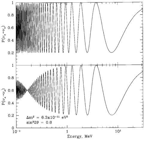
Although in the analyses [KP3, SPnu96] leading to the above results the predictions of the solar model [BP95] with heavy element diffusion for the fluxes of the pp, pep, ⁷Be, ⁸B and CNO neutrinos were used, it was also verified [KP3, BerRos, SPnu96] that the results so obtained (i.e., the existence of the vacuum $\nu_{e}\leftrightarrow\nu_{\mu(\tau)}$ oscillation solution) are stable with respect to variations of the values of the total ⁸B and ⁷Be neutrino fluxes within wide intervals in which the predictions of all contemporary solar models lie.

Figure 6: Regions of values of the parameters $\Delta m^{2}$ and $\sin^{2}2\theta$ (shown in black) for which the solar neutrino data can be described (at 95% C.L.) in terms of vacuum $\nu_{e}\leftrightarrow\nu_{\mu(\tau)}$ oscillations of the solar $\nu_{e}$ (from [72]). For further details see the text.

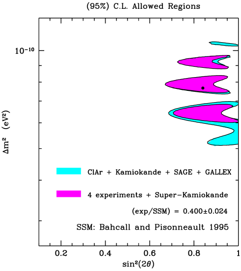
The results of a recent $\chi^{2}-$analysis of the solar neutrino data in terms of the hypothesis of two-neutrino $\nu_{e}\leftrightarrow\nu_{\mu(\tau)}$ oscillations of the solar neutrinos [PK97], are shown graphically in Fig. 6. The analysis was based on the predictions of the solar model of Bahcall and Pinsonneault [BP95] with heavy element diffusion. The regions in the $\Delta m^{2}-\sin^{2}2\theta$ plane colored in black correspond to values of the two parameters for which one obtains (at 95% C.L.) a description of the data, in other words, a solution of the solar neutrino problem.

Let us note that for the values of $\Delta m^{2}$ from the interval (28a), the oscillation length in vacuum for the solar neutrinos with energy $E\sim 1~{}{\rm MeV}$ is of the order of the Sun-Earth distance: ${L_{v}}\sim(2.5-5.0)\times 10^{7}~{}{\rm km}$. At the same time ${L_{v}}$ is much bigger than the solar radius: ${\rm L_{v}\gg R_{\odot}}$.

6.2 Matter-Enhanced Transitions

Let us consider next that the possible effects of the solar matter on the oscillations of solar neutrinos assuming that (18a) and (18b) hold true and supposing first that $|\nu_{x}\rangle\equiv|\nu_{\mu}\rangle$.

The presence of matter can drastically change the pattern of neutrino oscillations: neutrinos can interact with the particles forming the matter. Accordingly, the Hamiltonian of the neutrino system in matter differs from the Hamiltonian of the neutrino system in vacuum $H_{0}$,

$$H_{m}=H_{0}+H_{int}\,,~{}~{}$$

where $H_{int}$ describes the interaction of the flavour neutrinos with the particles of matter. When, e.g., electron neutrinos propagate in matter, they can scatter (due to the $H_{int}$) on the particles present in matter: on the electrons (e^-), protons ($p$) and neutrons ($n$). The incoherent elastic and the quasi-elastic scattering, in which the states of the initial particles change in the scattering process (destroying the coherence between the neutrino states), are not of interest for our discussion for one simple reason - they have a negligible effect on the solar neutrino propagation in the Sun  : even in the center of the Sun, where the density of matter is relatively high ($\sim 150~{}{\rm g/cm^{3}}$), an $\nu_{e}$ with energy of 1 MeV has a mean free path with respect to the indicated scattering processes, which exceeds $10^{10}~{}{\rm km}$ (recall that the solar radius is much smaller: ${\rm R_{\odot}}=6.96\times 10^{5}~{}{\rm km}$). The oscillating $\nu_{e}$ and $\nu_{\mu}$ can scatter also elastically in the forward direction on the e^-, $p$ and $n$, with the momenta and the spin states of the particles participating in the elastic scattering reaction remaining unchanged. In such a process the coherence of the neutrino states is being preserved and the oscillations between the flavour neutrinos can continue in spite of, and actually, in parallel to, the scattering.

The $\nu_{e}$ and $\nu_{\mu}$ coherent elastic scattering in the forward direction on the particles of matter generates nontrivial indices of refraction of the $\nu_{e}$ and $\nu_{\mu}$ in matter [MSW1]: $\kappa(\nu_{e})\neq 1$, $\kappa(\nu_{\mu})\neq 1$. Most importantly, the index of refraction of the $\nu_{e}$ thus generated does not coincide with the index of refraction of the $\nu_{\mu}$: $\kappa(\nu_{e})\neq\kappa(\nu_{\mu})$. The difference between the two indices of refraction is determined essentially by the difference of the real parts of the forward $\nu_{e}-e^{-}$ and $\nu_{\mu}-e^{-}$ elastic scattering amplitudes [MSW1], ${\rm Re~{}[F_{\nu_{e}-e^{-}}(0)]-Re~{}[F_{\nu_{\mu}-e^{-}}(0)]}$: due to the flavour symmetry of the neutrino – quark (neutrino – nucleon) neutral current interaction, the forward $\nu_{e}-p,n$ and $\nu_{\mu}-p,n$ elastic scattering amplitudes are equal and therefore do not contribute to the difference of interest. The real parts of the amplitudes ${\rm F_{\nu_{e}-e^{-}}(0)}$ and ${\rm F_{\nu_{\mu}-e^{-}}(0)}$ can be calculated in the standard theory. One finds the following result [MSW1, Barger80, Langa83] (see also [JLiu91]) for the difference of the indices of refraction of $\nu_{e}$ and $\nu_{\mu}$:

$$\kappa(\nu_{e})-\kappa(\nu_{\mu})={2\pi\over{p^{2}}}~{}\left({\rm Re~{}[F_{\nu_{e}-e^{-}}(0)]-Re~{}[F_{\nu_{\mu}-e^{-}}(0)]}\right)=-~{}{1\over{p}}\sqrt{2}G_{F}N_{e}~{},~{}$$

where $G_{F}$ is the Fermi constant and $N_{e}$ is the electron number density in matter. Let us note that the forward scattering amplitudes for the antineutrinos ${\rm F_{\bar{\nu}_{e}-e^{-}}(0)}$ and ${\rm F_{\bar{\nu}_{\mu}-e^{-}}(0)}$ coincide in absolute value with the amplitudes ${\rm F_{\nu_{e}-e^{-}}(0)}$ and ${\rm F_{\nu_{\mu}-e^{-}}(0)}$ but have opposite sign and therefore one has

$$\kappa(\bar{\nu}_{e})-\kappa(\bar{\nu}_{\mu})=+~{}{1\over{p}}\sqrt{2}\,G_{F}\,N_{e}~{}.~{}$$

Knowing the expression for the difference of the indices of refraction of $\nu_{e}$ and $\nu_{\mu}$ in matter, it is not difficult to write the system of evolution equations which describes the $\nu_{e}\leftrightarrow\nu_{\mu}$ oscillations in matter [MSW1, Barger80, Langa83]:

$$i\frac{d}{dt}\left(\begin{array}[]{c}A_{e}(t,t_{0})\\ A_{\mu}(t,t_{0})\end{array}\right)=\left(\begin{array}[]{cc}-\epsilon(t)&\epsilon^{\prime}\\ \epsilon^{\prime}&\epsilon(t)\end{array}\right)\left(\begin{array}[]{c}A_{e}(t,t_{0})\\ A_{\mu}(t,t_{0})\end{array}\right)~{}~{}$$

where $A_{e}(t,t_{0})$ ($A_{\mu}(t,t_{0})$) is the amplitude of the probability to find neutrino $\nu_{e}$ ($\nu_{\mu}$) at time $t$ of the evolution of the neutrino system if at time $t_{0}$ the neutrino $\nu_{e}$ or $\nu_{\mu}$ (or a state representing a linear combination of the states describing the two neutrinos) has been produced, $t\geq t_{0}$. Furthermore $\epsilon(t)$ and $\epsilon^{\prime}$ are real functions of the neutrino energy $E\cong p$, of $\Delta m^{2}$, of the mixing angle in vacuum $\theta$ and of the electron number density in the point of the neutrino trajectory in matter reached at time $t$, $N_{e}(t)$,

$$\epsilon(t)={1\over{2}}~{}[{~{}\Delta m^{2}\over{2E}}\cos 2\theta-\sqrt{2}G_{F}N_{e}(t)],~{}~{}\epsilon^{\prime}={\Delta m^{2}\over{4E}}\sin 2\theta.~{}~{}~{}$$

The term $\sqrt{2}G_{F}N_{e}(t)$ in the parameter $\epsilon(t)$ accounts for the effects of matter on the neutrino oscillations.

Let us note that the system of evolution equations describing the oscillations of antineutrinos $\bar{\nu}_{e}\leftrightarrow\bar{\nu}_{\mu}$ in matter has exactly the same form except for the matter term in $\epsilon(t)$ which, in accordance with (30) and (31), changes sign.

Due to the presence of the interaction term $H_{int}$ in the Hamiltonian of the neutrino system in matter $H_{m}$, the eigenstates of the Hamiltonian of the neutrino system in vacuum, $|\nu_{1}\rangle$ and $|\nu_{2}\rangle$, are not eigenstates of $H_{m}$. As a result of the coherent scattering of $\nu_{e}$ and $\nu_{\mu}$ off the particles forming the matter transitions between the states $|\nu_{1}\rangle$ and $|\nu_{2}\rangle$ become possible in matter:

$$\langle\nu_{2}|~{}H_{int}~{}|\nu_{1}\rangle~{}\neq~{}0.~{}~{}~{}$$

Consider first the case of $\nu_{e}\leftrightarrow\nu_{\mu}$ oscillations taking place in matter with electron number density which does not change along the neutrino trajectory: $N_{e}(t)=N_{e}=~{}const.$ It proves convenient to find the states $|\nu^{m}_{1,2}\rangle$, which diagonalize the evolution matrix in the right-hand side of the system (32), or equivalently, the Hamiltonian of the neutrino system in matter. The relations between the matter-eigenstates $|\nu^{m}_{1,2}\rangle$ and the flavour-eigenstates $|\nu_{e,\mu}\rangle$ have the same form as the relations (18a) and (18b) between the vacuum mass-eigenstates $|\nu_{1,2}\rangle$ and $|\nu_{e,\mu}\rangle$:

$$|\nu_{e}\rangle~{}=~{}~{}~{}|\nu^{m}_{1}\rangle\cos\theta_{m}+|\nu^{m}_{2}\rangle\sin\theta_{m},~{}~{}~{}$$

$$|\nu_{\mu}\rangle~{}~{}=-|\nu^{m}_{1}\rangle\sin\theta_{m}~{}+|\nu^{m}_{2}\rangle\cos\theta_{m}~{}.~{}~{}~{}$$

Here $\theta_{m}$ is the neutrino mixing angle in matter [MSW1],

$$\sin 2\theta_{m}={\epsilon^{\prime}\over{\sqrt{\epsilon^{2}+\epsilon^{\prime 2}}}}={\tan 2\theta\over{\sqrt{(1-{N_{e}\over{N_{e}^{res}}})^{2}+\tan^{2}2\theta}}},~{}~{}~{}$$

$$\cos 2\theta_{m}={\epsilon\over{\sqrt{\epsilon^{2}+\epsilon^{\prime 2}}}}={{1-N_{e}/N_{e}^{res}}\over{\sqrt{(1-{N_{e}\over{N_{e}^{res}}})^{2}+\tan^{2}2\theta}}},~{}~{}~{}$$

where the quantity

$$N_{e}^{res}={{\Delta m^{2}\cos 2\theta}\over{2E\sqrt{2}G_{F}}}~{}~{}~{}$$

is called “resonance density” [Barger80]. The matter-eigenstates $|\nu^{m}_{1,2}\rangle$ (which are also called “adiabatic”) are eigenstates of the evolution matrix (Hamiltonian) in (32), corresponding to the two eigenvalues, $E^{m}_{1,2}$, whose difference is given by

$$E^{m}_{2}-E^{m}_{1}=2\sqrt{\epsilon^{2}+\epsilon^{\prime 2}}={\Delta m^{2}\over{2E}}~{}\sqrt{(1-{N_{e}\over{N_{e}^{res}}})^{2}\cos^{2}2\theta+\sin^{2}2\theta}.~{}~{}~{}$$

It should be almost obvious from (25) after comparing (18a), (18b) with (35a), (35b) that the probability to find neutrino $\nu_{\mu}$ at time $t$ if neutrino $\nu_{e}$ has been produced at time $t_{0}=0$ and it traversed a distance $(t-t_{0})=t\cong R_{m}$ in matter with constant electron number density $N_{e}$, has the form [MSW2]:

$$P_{m}(\nu_{e}\rightarrow\nu_{\mu};t)=|A_{\mu}(t)|^{2}={1\over 2}\sin^{2}2\theta_{m}~{}\left[1-\cos 2\pi{R_{m}\over L_{m}}\right],~{}~{}~{}$$

where

$$2\pi{R_{m}\over L_{m}}\cong(E^{m}_{2}-E^{m}_{1})t,~{}~{}$$

and $L_{m}$ is the oscillation length in matter:

$$L_{m}={L_{v}\over{\sqrt{(1-{N_{e}\over{N_{e}^{res}}})^{2}\cos^{2}2\theta+\sin^{2}2\theta}}}\,.~{}$$

Evidently, the amplitude of the $\nu_{e}\leftrightarrow\nu_{\mu}$ oscillations in matter is equal to $\sin^{2}2\theta_{m}$. It follows from (36) that, most remarkably, the dependence of $\sin^{2}2\theta_{m}$ on $N_{e}$ has a resonance character [MSW2]. Indeed, if in the case of interest the condition

$$\Delta m^{2}\cos^{2}2\theta>0~{}~{}~{}$$

is fulfilled, for any finite value of $\sin^{2}2\theta$ there exists a value of the electron number density equal to $N_{e}^{res}$, such that when

$$N_{e}=N_{e}^{res}~{}~{}$$

we have

$$\sin^{2}2\theta_{m}=1\,.~{}~{}$$

Note that if $N_{e}=N_{e}^{res}$, we get $\sin^{2}2\theta_{m}=1$ even if the mixing angle in vacuum is small, i.e., if $\sin^{2}2\theta\ll 1$. This implies that the presence of matter can lead to a strong enhancement of the oscillation probability $P_{m}(\nu_{e}\rightarrow\nu_{\mu};t)$ even when the $\nu_{e}\leftrightarrow\nu_{\mu}$ oscillations in vacuum are strongly suppressed due to a small value of $\sin^{2}2\theta$ (hence, the name “matter-enhanced neutrino oscillations”).

The oscillation length at resonance is given by

$$L^{res}_{m}={L_{v}\over{\sin 2\theta}}\,,~{}$$

while the width in $N_{e}$ of the resonance (i.e., the “distance” in $N_{e}$ between the points at which $\sin^{2}2\theta_{m}=1/2$) has the form

$$\Delta N_{e}^{res}=2N_{e}^{res}\tan 2\theta~{}.~{}$$

Thus, if the mixing angle in vacuum is small the resonance is narrow, $\Delta N_{e}^{res}\ll N_{e}^{res}$, and the oscillation length in matter at resonance is relatively large, $L^{res}_{m}\gg L_{v}$. As it follows from (39), the energy difference $E^{m}_{2}-E^{m}_{1}$ has a minimum at the resonance:

$$(E^{m}_{2}-E^{m}_{1})^{res}={\rm min}~{}(E^{m}_{2}-E^{m}_{1})={\Delta m^{2}\over{2E}}~{}\sin 2\theta.~{}~{}~{}$$

It is instructive to consider two limiting case. If $N_{e}\ll N_{e}^{res}$, as it follows from (36) and (42), $\theta_{m}\cong\theta$ ($\sin 2\theta_{m}\cong\sin 2\theta$), ${\rm L_{m}}\cong{{\rm L_{v}}}$ and the neutrinos oscillate practically as in vacuum. In the opposite limit, $N_{e}\gg N_{e}^{res},~{}N_{e}^{res}\tan^{2}2\theta$, one finds from (36) and (37) that $\theta_{m}\cong\pi/2$ ($\sin 2\theta_{m}\cong 0$, $\cos 2\theta_{m}\cong-1$) and the presence of matter suppresses the $\nu_{e}\leftrightarrow\nu_{\mu}$ oscillations (see (40)). In this case we get from (35a) and (35b):

$$|\nu_{e}\rangle~{}\cong~{}~{}~{}|\nu^{m}_{2}\rangle,~{}~{}~{}$$

$$|\nu_{\mu}\rangle~{}=-|\nu^{m}_{1}\rangle,~{}~{}~{}$$

i.e., if the electron number density exceeds considerably the resonance density, $\nu_{e}$ practically coincides with the heavier of the two matter-eigenstate neutrinos $\nu^{m}_{2}$, while the $\nu_{\mu}$ coincides with the lighter one $\nu^{m}_{1}$.

The analogs of (36), (37), (39), (40) and (42) for oscillations of antineutrinos, $\bar{\nu}_{e}\leftrightarrow\bar{\nu}_{\mu}$, in matter with constant $N_{e}$ can formally be obtained by replacing $N_{e}$ with $(-N_{e})$ in the indicated equations. If condition (43) is fulfilled, we have $N_{e}^{res}>0$ and the term $(1+N_{e}/N_{e}^{res})$ which appears, e.g., in the expression for the mixing angle in matter $\bar{\theta}_{m}$ in the case of $\bar{\nu}_{e}\leftrightarrow\bar{\nu}_{\mu}$ oscillations, can never be zero. Thus, a resonance enhancement of the $\bar{\nu}_{e}\leftrightarrow\bar{\nu}_{\mu}$ oscillations cannot take place. The matter, actually, can only suppress the oscillations.

It should be clear from this discussion that depending on the sign of the product $\Delta m^{2}~{}\cos 2\theta$, the presence of matter can lead to resonance enhancement either of the $\nu_{e}\leftrightarrow\nu_{\mu}$ or of the $\bar{\nu}_{e}\leftrightarrow\bar{\nu}_{\mu}$ oscillations, but not of the both types of oscillations. This is a consequence of the fact [LangP] that the matter in the Sun or in the Earth we are interested in, is not charge-symmetric (it contains $e^{-},~{}p$ and $n$, but does not contain their antiparticles) and therefore the oscillations in matter are neither CP- nor CPT- invariant. In what follows we shall assume that $\Delta m^{2}>0$ and $\cos 2\theta>0$, so that (43) is satisfied and therefore only the $\nu_{e}\leftrightarrow\nu_{\mu}$ oscillations can be enhanced by the matter effects.

Since the neutral current weak interaction of neutrinos in the standard theory is flavour symmetric, the formulae and results we have obtained above and shall obtain in what follows are valid for the case of $\nu_{e}-\nu_{\tau}$ mixing ((18a) and (18b)) and $\nu_{e}\leftrightarrow\nu_{\tau}$ oscillations in matter as well. In what concerns the possibility of mixing and oscillations between the $\nu_{e}$ and a sterile neutrino $\nu_{s}$, $\nu_{e}\leftrightarrow\nu_{s}$, the relevant formulae can be obtained from the formulae derived for the case of $\nu_{e}\leftrightarrow\nu_{\mu(\tau)}$ oscillations by [LangP] replacing $N_{e}$ with $(N_{e}-1/2N_{n})$, where $N_{n}$ is the number density of neutrons in matter.

The formalism we have developed above can be directly applied, for instance, to the study of the matter effects in the $\nu_{e}\leftrightarrow\nu_{\mu(\tau)}$ ($\nu_{\mu(\tau)}\leftrightarrow\nu_{e}$) oscillations of the flavour neutrinos which traverse the Earth mantle (but do not traverse the Earth core). The electron number density changes little around the mean value of $\bar{N}_{e}\cong 2.3~{}cm^{-3}~{}N_{A}$, $N_{A}$ being the Avogadro number, along the trajectories of neutrinos which cross a substantial part of the Earth mantle and the $N_{e}=const.$ approximation is rather accurate. If, for example, $\Delta m^{2}=10^{-3}~{}{\rm eV^{2}}$, $E=1~{}{\rm GeV}$ and $\sin^{2}2\theta\cong 0.5$, we have: $N_{e}^{res}\cong 4.6~{}cm^{-3}~{}N_{A}$, $\sin^{2}2\theta_{m}\cong 0.8$ and the oscillation length in matter, $L_{m}\cong 3\times 10^{3}~{}{\rm km}$, is of the order of the depth of the Earth mantle, so that one can have $2\pi R_{m}\ga L_{m}$. It is not difficult to obtain an expression for the $\nu_{e}\leftrightarrow\nu_{\mu(\tau)}$ oscillation probability in the case when the neutrinos traverse both the Earth mantle and the core assuming ${N_{e}}$ is constant, but has different values in the two Earth density structures.

It is not clear, however, what the above interesting results have to do with the problem of main interest for us, namely, accounting for the effects of solar matter in the oscillations of solar neutrinos while they propagate from the central part to the surface of the Sun. The electron number density (the matter density) changes considerably along the neutrino path in the Sun: it decreases monotonically from the value of $\sim 100~{}{\rm cm^{-3}}~{}N_{A}$ ($\sim 150~{}{\rm g/cm^{3}}$) in the center of the Sun to 0 at the surface of the Sun. Actually, according to the contemporary solar models (see, e.g., [JNB, BP95]), $N_{e}$ decreases approximately exponentially in the radial direction towards the surface of the Sun:

$$N_{e}(t)=N_{e}(t_{0})\exp{\left\{-{{t-t_{0}}\over{r_{0}}}\right\}},~{}~{}~{}~{}~{}$$

where $(t-t_{0})\cong d$ is the distance traveled by the neutrino in the Sun, $N_{e}(t_{0})$ is the electron number density in the point of neutrino production in the Sun, $r_{0}$ is the scale-height of the change of $N_{e}(t)$ and one has [JNB]  $r_{0}\sim 0.1R_{\odot}$.

Obviously, if $N_{e}$ changes with $t$ (or equivalently with the distance) along the neutrino trajectory, the matter-eigenstates, their energies, the mixing angle and the oscillation length in matter, become, through their dependence on $N_{e}$, also functions of $t$: $|\nu^{m}_{1,2}\rangle=|\nu^{m}_{1,2}(t)\rangle$, $E^{m}_{1,2}=E^{m}_{1,2}(t)$, $\theta_{m}=\theta_{m}(t)$ and $L_{m}=L_{m}(t)$.

It is not difficult to understand qualitatively the possible behaviour of the neutrino system when solar neutrinos propagate from the center to the surface of the Sun if one realizes that one is dealing effectively with a two-level system whose Hamiltonian depends on time and admits“jumps” from one level to the other (see (32)). Let us assume first for simplicity that the electron number density in the point of a solar $\nu_{e}$ production in the Sun is much bigger than the resonance density, $N_{e}(t_{0})\gg N_{e}^{res}$, and that the mixing angle in vacuum is small, $\sin\theta\ll 1$. Actually, this is one of the cases relevant to the solar neutrinos. In this case we have $\theta_{m}(t_{0})\cong\pi/2$ and the state of the electron neutrino in the initial moment of the evolution of the system practically coincides with the heavier of the two matter-eigenstates:

$$|\nu_{e}\rangle~{}\cong~{}~{}~{}|\nu^{m}_{2}(t_{0})\rangle.~{}~{}~{}$$

Thus, at $t_{0}$ the neutrino system is in a state corresponding to the “level” with energy $E^{m}_{2}(t_{0})$. When neutrinos propagate to the surface of the Sun they cross a layer of matter in which $N_{e}=N_{e}^{res}$: in this layer the difference between the energies of the two “levels” $(E^{m}_{2}(t)-E^{m}_{1}(t))$ has a minimal value on the neutrino trajectory ( (39) and (40)). Correspondingly, the evolution of the neutrino system can proceed basically in two ways. First, the system can stay on the “level” with energy $E^{m}_{2}(t)$, i.e., can continue to be in the state $|\nu^{m}_{2}(t)\rangle$ up to the final moment $t_{s}$, when the neutrino reaches the surface of the Sun. At the surface of the Sun $N_{e}(t_{s})=0$ and therefore $\theta_{m}(t_{s})=\theta$, $|\nu^{m}_{1,2}(t_{s})\rangle\equiv|\nu_{1,2}\rangle$ and $E^{m}_{1,2}(t_{s})=E_{1,2}$. Thus, in this case the state describing the neutrino system at $t_{0}$ will evolve continuously into the state $|\nu_{2}\rangle$ at the surface of the Sun. Using (18a) and (18b), it is trivial to obtain now the probabilities to find respectively neutrino $\nu_{e}$ and neutrino $\nu_{\mu}$ at the surface of the Sun (given the fact that $\nu_{e}$ has been produced in the initial point of the neutrino trajectory):

$$P(\nu_{e}\rightarrow\nu_{e};t_{s},t_{0})\equiv|A_{e}(t_{s},t_{0})|^{2}\cong|\langle\nu_{e}|\nu_{2}\rangle|^{2}=\sin^{2}\theta,~{}~{}$$

$$P(\nu_{e}\rightarrow\nu_{\mu};t_{s},t_{0})\equiv|A_{\mu}(t_{s},t_{0})|^{2}\cong|\langle\nu_{\mu}|\nu_{2}\rangle|^{2}=\cos^{2}\theta.~{}~{}$$

It is clear that under the assumptions made (i.e., $\sin^{2}\theta\ll 1$), a practically total $\nu_{e}-\nu_{\mu}$ conversion is possible in the case under study. This type of evolution of the neutrino system as well as the $\nu_{e}\rightarrow\nu_{\mu}$ transitions taking place during the evolution, are called [MSW2] “adiabatic”. They are characterized by the fact that the probability of the “jump” from the upper “level” (having energy $E^{m}_{2}(t)$) to the lower “level” (with energy $E^{m}_{1}(t)$), $P^{\prime}$, or equivalently the probability of the $\nu^{m}_{2}(t_{0})\rightarrow\nu^{m}_{1}(t_{s})$ transition, $P^{\prime}\equiv P^{\prime}(\nu^{m}_{2}(t_{0})\rightarrow\nu^{m}_{1}(t_{s}))$, on the whole neutrino trajectory is negligible:

$$P^{\prime}\equiv P^{\prime}(\nu^{m}_{2}(t_{0})\rightarrow\nu^{m}_{1}(t_{s}))\cong 0~{}:~{}adiabatic~{}transitions.~{}~{}$$

The second possibility is realized if in the resonance region, where the two “levels” approach each other most (the difference between the energies of the two “levels” $(E^{m}_{2}(t)-E^{m}_{1}(t))$ has a minimal value), the system “jumps” from the upper “level” to the lower “level” and after that continues to be in the state $|\nu^{m}_{1}(t)\rangle$ until the neutrino reaches the surface of the Sun. Evidently, now we have $P^{\prime}\equiv P^{\prime}(\nu^{m}_{2}(t_{0})\rightarrow\nu^{m}_{1}(t_{s}))\cong 1$. In this case the neutrino system ends up in the state $|\nu^{m}_{1}(t_{s})\rangle\equiv|\nu_{1}\rangle$ at the surface of the Sun and the probabilities to find the neutrinos $\nu_{e}$ and $\nu_{\mu}$ at the surface of the Sun are given by

$$P(\nu_{e}\rightarrow\nu_{e};t_{s},t_{0})\equiv|A_{e}(t_{s},t_{0})|^{2}\cong|\langle\nu_{e}|\nu_{1}\rangle|^{2}=\cos^{2}\theta,~{}~{}$$

$$P(\nu_{e}\rightarrow\nu_{\mu};t_{s},t_{0})\equiv|A_{\mu}(t_{s},t_{0})|^{2}\cong|\langle\nu_{\mu}|\nu_{1}\rangle|^{2}=\sin^{2}\theta.~{}~{}$$

Obviously, if $\sin^{2}\theta\ll 1$, practically no transitions of the solar $\nu_{e}$ into $\nu_{\mu}$ will occur. The considered regime of evolution of the neutrino system and the corresponding $\nu_{e}\rightarrow\nu_{\mu}$ transitions are usually referred to as “extremely nonadiabatic”.

Clearly, the value of the “jump” probability $P^{\prime}$ plays a crucial role in the the $\nu_{e}\rightarrow\nu_{\mu}$ transitions: it fixes the type of the transition and determines to large extent $\nu_{e}\rightarrow\nu_{\mu}$ transition probability. We have considered above two limiting cases: $P^{\prime}\cong 0$ and $P^{\prime}\cong 1$. Obviously, there exists a whole spectrum of possibilities since $P^{\prime}$ can have any value from 0 to 1. In general, the transitions are called “nonadiabatic” if $P^{\prime}$ is non-negligible (see further).

Numerical studies have shown [MSW2] that solar neutrinos can undergo both adiabatic and nonadiabatic $\nu_{e}\rightarrow\nu_{\mu}$ transitions in the Sun and the matter effects can be substantial in the solar neutrino oscillations for a remarkably wide range of values of the two parameters $\Delta m^{2}$ and $\sin^{2}2\theta$, namely for

$$10^{-7}{\rm eV}^{2}\la\Delta m^{2}\la 10^{-4}{\rm eV}^{2},~{}~{}$$

$$10^{-4}\la\sin^{2}2\theta\leq 1.0\,.~{}~{}~{}$$

It would be preferable to make more quantitative the preceding analysis. We will obtain first the adiabaticity condition [MSW2, Messiah86].

Using the (35a) and (35b) we can express the probability amplitudes $A_{e}(t,t_{0})$ and $A_{\mu}(t,t_{0})$ in terms of the probability amplitudes $A_{1}(t,t_{0})$ and $A_{2}(t,t_{0})$ to find the neutrino system in the states $|\nu^{m}_{1}(t)\rangle$ and $|\nu^{m}_{2}(t))\rangle$, respectively, at time $t$:

$$A_{e}(t,t_{0})~{}=~{}~{}~{}A_{1}(t,t_{0})\cos\theta_{m}(t)+A_{2}(t,t_{0})\sin\theta_{m}(t),~{}~{}~{}$$

$$A_{\mu}(t,t_{0})~{}=-A_{1}(t,t_{0})\sin\theta_{m}(t)+A_{2}(t,t_{0})\cos\theta_{m}(t).~{}~{}~{}$$

Substituting (56a) and (56b) in (32) we obtain the system of evolution equations for the probability amplitudes $A_{1}(t,t_{0})$ and $A_{2}(t,t_{0})$:

$$i\frac{d}{dt}\left(\begin{array}[]{c}A_{1}(t,t_{0})\\ A_{2}(t,t_{0})\end{array}\right)=\left(\begin{array}[]{cc}E_{1}^{m}(t)&-i\dot{\theta}_{m}(t)\\ i\dot{\theta}_{m}(t)&E_{2}^{m}(t)\end{array}\right)\left(\begin{array}[]{c}A_{1}(t,t_{0})\\ A_{2}(t,t_{0})\end{array}\right)\,.~{}~{}$$

Here $\dot{\theta}_{m}(t)\equiv{d\over{dt}}\theta_{m}(t)$. It follows from the preceding discussion that the solar neutrino transitions in the Sun will be adiabatic (nonadiabatic) if the nondiagonal term in the evolution matrix in the right-hand side of (57), which is responsible for the $\nu^{m}_{2}(t_{0})\rightarrow\nu^{m}_{1}(t_{s})$ transitions, is sufficiently small (is non-negligible). The corresponding conditions can be written as

$$4n(t)\gg 1,~{}~{}~{}~{}~{}adiabatic~{}~{}transitions,~{}~{}~{}~{}~{}~{}~{}~{}$$

$$4n(t)\la 1,~{}~{}~{}~{}~{}nonadiabatic~{}~{}transitions,~{}~{}$$

where the adiabaticity function $4n(t)$ is given by

$$4n(t)\equiv{{E^{m}_{2}(t)-E^{m}_{1}(t)}\over{2|\dot{\theta}_{m}(t)|}}=\sqrt{2}G_{F}{{(N^{res}_{e})^{2}}\over{|\dot{N}_{e}(t)|}}\tan^{2}2\theta\left(1+tan^{-2}2\theta_{m}(t)\right)^{\frac{3}{2}}~{}.~{}~{}$$

In (59) $\dot{N}_{e}(t)\equiv{d\over{dt}}N_{e}(t)$ and we have used (36), (37) and (39) to derive it. Expression (59) for $4n(t)$ implies that the solar neutrino transitions in the Sun will be adiabatic if the electron number density changes sufficiently slowly along the neutrino trajectory; if the change of $N_{e}(t)$ is relatively fast, the transitions would be nonadiabatic.

In order for the solar neutrino transitions to be, e.g., adiabatic, condition (58a) has to be fulfilled in any point of neutrino trajectory in the Sun. However, it is not difficult to convince oneself using (36), (37), (50) and (59) that if the solar neutrinos cross a layer with resonance density $N_{e}^{res}$ on their way to the surface of the Sun, condition (58a) will hold if it holds at the resonance point, i.e., for the parameter

$$\begin{array}[]{rcl}4n_{0}\equiv 4n(t=t_{res})&=&\displaystyle\sqrt{2}G_{F}{{(N^{res}_{e})^{2}}\over{|\dot{N}_{e}(t=t_{res})|}}\tan^{2}2\theta\vspace{2mm}\\ &=&\displaystyle r_{0}~{}{\Delta m^{2}\over{2E}}~{}{\sin^{2}2\theta\over{\cos 2\theta}}=\pi~{}{\Delta r^{res}\over{L_{m}^{res}}}\,,\end{array}~{}~{}$$

where $t_{res}$ is the time at which the resonance layer is crossed by the neutrinos, $t_{0}<t_{res}<t_{s}$, $\Delta r^{res}=2(N^{res}_{e}/|\dot{N}_{e}(t=t_{res})|)\tan 2\theta\cong 2r_{0}~{}\tan 2\theta$ is the spatial width of the resonance and we have used (38) and (46). Thus, the value of the adiabaticity parameter $4n_{0}$ determines the type of the solar neutrino transitions. It follows from (60), in particular, that the transitions will be adiabatic if the width of the resonance is bigger than the oscillation length at resonance.

Actually, the system of evolution equations (32) can be solved exactly in the case when $N_{e}$ changes exponentially, (50), along the neutrino path in the Sun [SP200, EXP]. On the basis of the exact solution, which is expressed in terms of confluent hypergeometric functions [BE], it was possible to derive a complete, simple and very accurate analytic description of the matter-enhanced transitions of solar neutrinos in the Sun [SP200], [SP191]–[SPJR89] (for a review see [SP90]). The probability that a $\nu_{e}$ having momentum p (or energy ${\rm E\cong p}$) and produced at time t₀ in the central part of the Sun will not transform into $\nu_{\mu(\tau)}$ on its way to the surface of the Sun (reached at time t_s) is given by

$$P_{\odot}(\nu_{e}\rightarrow\nu_{e};t_{s},t_{0})=\bar{P}_{\odot}(\nu_{e}\rightarrow\nu_{e};t_{s},t_{0})+~{}Oscillating~{}terms.~{}~{}$$

Here

$$\bar{P}_{\odot}(\nu_{e}\rightarrow\nu_{e};t_{s},t_{0})\equiv\bar{P}_{\odot}={1\over 2}+\left({1\over 2}-{\rm P}^{{}^{\prime}}\right)\cos 2\theta_{m}(t_{0})\cos 2\theta~{}$$

is the average probability, where

$$P^{{}^{\prime}}={{\exp\left[-2\pi{\rm r}_{0}{\Delta m^{2}\over{2E}}\sin^{2}\theta\right]-\exp\left[-2\pi{\rm r}_{0}{\Delta m^{2}\over{2E}}\right]}\over{1-\exp\left[-2\pi{\rm r}_{0}{\Delta m^{2}\over{2E}}\right]}}~{}~{}~{}~{}~{}~{}~{}~{}~{}~{}~{}~{}~{}~{}~{}~{}~{}~{}~{}~{}~{}~{}~{}~{}~{}~{}~{}~{}~{}~{}~{}$$

$$=~{}{{\exp\left[-2\pi n_{0}(1-\tan^{2}\theta)\right]-\exp\left[-2\pi n_{0}(\tan^{-2}\theta-\tan^{2}\theta)\right]}\over{1-\exp\left[-2\pi n_{0}(\tan^{-2}\theta-\tan^{2}\theta)\right]}}~{},~{}~{}$$

is [SP200, SP90] the “jump” probability for exponentially varying electron number density  $N_{e}$, and $\theta_{m}(t_{0})$ is the neutrino mixing angle in matter in the point of $\nu_{e}$ production.

We will not give the explicit analytic expressions for the oscillating terms in the probability $P_{\odot}(\nu_{e}\rightarrow\nu_{e};t_{s},t_{0})$, although they have been derived in the exponential density approximation for the $N_{e}$ as well [SP88osc] (see also [SP97]). These terms were shown [SPJR89] to be, in general, strongly suppressed by the various averagings one has to perform when analyzing the solar neutrino data in terms of the hypothesis that solar neutrinos undergo matter-enhanced transitions in the Sun. More specifically, it was found [SPJR89] that the oscillating terms in $P_{\odot}(\nu_{e}\rightarrow\nu_{e};t_{s},t_{0})$ can be important only for the monochromatic ⁷Be– and pep–neutrinos and only for values of $\Delta m^{2}\la 10^{-8}~{}{\rm eV^{2}}$. As we shall see, the current solar neutrino data suggest that $\Delta m^{2}\ga 10^{-7}~{}{\rm eV^{2}}$.

It should be emphasized that for $\Delta m^{2}\ga 10^{-7}~{}{\rm eV^{2}}$ the averaging over the region of solar neutrino production in the Sun and the integration over the neutrino energy renders negligible all interference terms which appear in the probability of $\nu_{e}$ survival due to the $\nu_{e}\leftrightarrow\nu_{\mu(\tau)}$ oscillations in vacuum taking place on the way of the neutrinos from the surface of the Sun to the surface of the Earth. Thus, the probability that $\nu_{e}$ will remain $\nu_{e}$ while it travels from the central part of the Sun to the surface of the Earth is effectively equal to the probability of survival of the $\nu_{e}$ while it propagates from the central part of the Sun to the surface of the Sun and is given by the average probability $\bar{P}_{\odot}(\nu_{e}\rightarrow\nu_{e};t_{s},t_{0})$ (determined by (62) and (63)).

The probability $\bar{P}_{\odot}(\nu_{e}\rightarrow\nu_{e};t_{s},t_{0})$ has several interesting properties. If the solar $\nu_{e}$ transitions are adiabatic (i.e., $P^{\prime}\cong 0$) and $\cos 2\theta_{m}(t_{0})\cong-1$ (i.e., $N_{e}(t_{0})/N_{e}^{res}\gg 1,\tan 2\theta$, solar neutrinos are born “above” and “far” (in $N_{e}$) from the resonance region), one has

$$\bar{P}(\nu_{e}\rightarrow\nu_{e};t_{s},t_{0})\cong\sin^{2}\theta,~{}~{}~{}$$

which is compatible with the qualitative result (52a) derived earlier. The solar $\nu_{e}$ undergo extreme nonadiabatic transitions in the Sun ($4n_{0}\ll 1$) if, e.g., $E/\Delta m^{2}$ is “large” (see (60)). In this case again $\cos 2\theta_{m}(t_{0})\cong-1$ and, as it follows [SP200] from (63), $P^{\prime}\cong\cos^{2}\theta$. Correspondingly, the average probability takes the form:

$$\bar{P}(\nu_{e}\rightarrow\nu_{e};t_{s},t_{0})\cong 1-{1\over{2}}\sin^{2}2\theta~{},~{}~{}$$

which is the average two-neutrino vacuum oscillation probability. Thus, if the solar neutrino transitions are extremely nonadiabatic, the $\nu_{e}$ undergo oscillations in the Sun as in vacuum. We get the same result, eq. (65), if $N_{e}(t_{0})(1-\tan 2\theta)^{-1}<N_{e}^{res}$, i.e., when $E/\Delta m^{2}$ is sufficiently small so that the resonance density exceeds the density in the point of neutrino production. In this case [KP88] the $\nu_{e}$ transitions are adiabatic ($P^{\prime}\cong 0$) and again the $\nu_{e}\leftrightarrow\nu_{\mu(\tau)}$ oscillations take place in the Sun as in vacuum: $\cos 2\theta_{m}(t_{0})\cong\cos 2\theta$ and $\bar{P}(\nu_{e}\rightarrow\nu_{e};t_{s},t_{0})\cong 1-{1\over{2}}\sin^{2}2\theta$.

Let us note that the general aspects of the discussion and the results presented above are valid also in the case of solar neutrino transitions into sterile neutrino, $\nu_{e}\rightarrow\nu_{s}$. In particular, the average probability $\bar{P}_{\odot}(\nu_{e}\rightarrow\nu_{e};t_{s},t_{0})$ in this case is given effectively by (62) and (63) with [LangP] $N_{e}(t_{0})$ replaced by $(N_{e}(t_{0})-1/2N_{n}(t_{0}))$ in the expression for $\cos 2\theta_{m}(t_{0})$, $N_{n}(t_{0})$ being the neutron number density of neutrons in the point of neutrino production in the Sun.

The probability $\bar{P}(\nu_{e}\rightarrow\nu_{e};t_{s},t_{0})$ is shown as function of $E/\Delta m^{2}$ for three values of $\sin^{2}2\theta=0.8;~{}0.2;~{}5\times 10^{-3}$ in Figs. 7a - 7c.

Figure 7: (c)The solar $\nu_{e}$ survival probability [90]$\bar{P}_{\odot}(\nu_{e}\rightarrow\nu_{e};t_{s},t_{0})$, Eq. (62), averaged over the region of production the pp (solid line), pep (long-dash-dotted line), ¹³N (dashed line), ⁷Be (dash-dotted line), ¹⁵O (long-dashed line) and ⁸B (dotted line) neutrinos for $\sin^{2}2\theta=0.8~{}(a);~{}0.2~{}(b);~{}0.005~{}(c)$ as a function of $E/\Delta m^{2}$. Figures a and b correspond to $\nu_{e}\rightarrow\nu_{\mu(\tau)}$ transitions, while figure c corresponds to $\nu_{e}\rightarrow\nu_{s}$ transitions.

Fig. 7 (c)

Further details concerning the analytic description of the matter–enhanced transitions of the solar neutrinos in the Sun can be found in [SP200], [SP191]–[SP90], [LINEAR, SP97]. Exact analytic results for the probability of various possible two-neutrino matter-enhanced transitions in a medium ($\nu_{e}\rightarrow\nu_{\mu(\tau)}$ or the inverse, $\nu_{e}\rightarrow\nu_{\bar{\mu}(\bar{\tau})}$ or the inverse, $\bar{\nu}_{e}\rightarrow\nu_{\mu(\tau)}$ or the inverse, $\nu_{\mu}\rightarrow\nu_{s}$, etc.), which are based solely on the general properties of the system of evolution equations (32) (and do not make use of the explicit form of the functions $\epsilon(t)$ and $\epsilon^{\prime}(t))$ are given in [SP97].

Earlier studies (from 1993 – 1994) of the possibility to explain the solar neutrino problem in terms of the hypothesis of matter–enhanced $\nu_{e}\rightarrow\nu_{\mu(\tau)}$ transitions of solar neutrinos have shown [KP4] that the data admits, in general, two types of MSW solutions: a small mixing angle nonadiabatic solution for $10^{-3}<\sin^{2}2\theta\la 10^{-2}$, and a large mixing angle adiabatic one for approximately $0.60\la\sin^{2}2\theta\la 0.95$, with the allowed values of $\Delta m^{2}$ lying in the interval $10^{-7}~{}{\rm eV^{2}}\la\Delta m^{2}\la 10^{-4}~{}{\rm eV^{2}}$. The terms “nonadiabatic” and “adiabatic” refer to the type of transitions the ⁸B neutrinos undergo in the corresponding cases. It was also shown (see, e.g., [KP2, KP5]) that in the case of $\nu_{e}\rightarrow\nu_{s}$ transitions only a small mixing angle nonadiabatic solution, analogous to the $\nu_{e}\rightarrow\nu_{\mu(\tau)}$ nonadiabatic solution, is allowed by the data.

Recently the MSW solutions of the solar neutrino problem have been re-examined [PK97, SPnu96, SPHeid97]  (exploiting the $\chi^{2}-$method) using the data (1), (2), and (4), the GALLEX result from 51 runs of measurements, $\bar{\rm R}_{\rm GALLEX}({\rm Ge})=(69.7~{}\pm 6.7^{+~{}3.9}_{-~{}4.5})\hskip 5.69046pt{\rm SNU}$, and the Super-Kamiokande result from 201.6 days of measurements ($\sim 3000$ events), $\Phi^{{\rm SK}}_{{\rm B}}=(2.65~{}~{}^{+0.09}_{-0.08}~{}~{}^{+0.14}_{-0.10})\times 10^{6}~{}\nu_{e}/cm^{2}/sec~{}$. The analysis was based on the predictions of the solar model of [BP95] with heavy element diffusion for the electron and neutron number density distributions and for the relevant pp, pep, ⁷Be, ⁸B and CNO components of the solar neutrino flux. The uncertainties in the predictions for the fluxes estimated in [BP95] as well as the uncertainties of the different solar neutrino detection reaction cross-sections were taken into account. The probability $\bar{P}_{\odot}(\nu_{e}\rightarrow\nu_{e};t_{s},t_{0})$ was calculated following the prescriptions given in [KP88]. The results obtained in the cases of $\nu_{e}\rightarrow\nu_{\mu(\tau)}$ and $\nu_{e}\rightarrow\nu_{s}$ transitions are depicted in Figs. 8 and 9, respectively.

Figure 8: Regions of values of the parameters $\Delta m^{2}$ and $\sin^{2}2\theta$ (the black areas) for which the matter-enhanced $\nu_{e}\rightarrow\nu_{\mu(\tau)}$ transitions of solar $\nu_{e}$ allows to describe (at 95% C.L.) the solar neutrino data (from [72]). For further details see the text.

Figure 9: Allowed region of values of the parameters $\Delta m^{2}$ and $\sin^{2}2\theta$ corresponding to the matter-enhanced $\nu_{e}\rightarrow\nu_{s}$ transition solution of the solar neutrino problem (from [72]). For further details see the text.

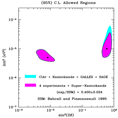
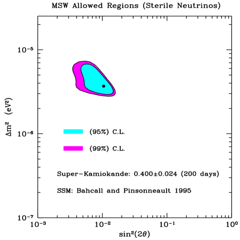
The solid line contours in Fig. 8 denote regions allowed by the data from the Homestake, Kamiokande, SAGE and GALLEX experiments, while the dark shaded regions have been obtained by including the Super-Kamiokande data in the analysis. Thus, the dark shaded areas represent the regions allowed by the mean event rate data from all experiments. The solid line contours in Fig. 9 denote the region allowed by the data (at 95% and at 99% C.L.).

The current solar neutrino data are best described assuming the solar neutrinos undergo small mixing angle $\nu_{e}\rightarrow\nu_{\mu(\tau)}$ matter-enhanced transitions [PK97, SPnu96, SPHeid97]  (for this nonadiabatic solution one has $\chi^{2}_{min}=0.9$ (3 d.f.)). The quality of the fit of the data is somewhat worse in the case of the large mixing angle or adiabatic solution ($\chi^{2}_{min}$ is somewhat larger: $\chi^{2}_{min}=1.5$). A similar quality of the fit of the data is provided also by the hypothesis of transitions into a sterile neutrino, $\nu_{e}\rightarrow\nu_{s}$, at small mixing angles ($\chi^{2}_{min}=1.5$). In contrast, the large mixing angle $\nu_{e}\rightarrow\nu_{s}$ transition solution is practically excluded as a possible explanation of the solar neutrino deficit [PK97, SPnu96, SPHeid97]  (it is ruled out at 99.98% C.L. ($\chi^{2}_{min}=21$, 3 d.f.) by the data).

The values of the parameters $\Delta m^{2}$ and $\sin^{2}2\theta$ for which one obtains (at 95% C.L.) the small mixing angle $\nu_{e}\rightarrow\nu_{\mu(\tau)}$ transition solution of the solar neutrino problem lie in the region:

$$3.8\times 10^{-6}{\rm eV}^{2}\la\Delta m^{2}\la 10^{-5}{\rm eV}^{2},~{}~{}$$

$$3.5\times 10^{-3}\la\sin^{2}2\theta\la 1.4\times 10^{-2}.~{}~{}~{}$$

As Figs. 7 and 8 show, the small mixing angle $\nu_{e}\rightarrow\nu_{s}$ solution region is very similar in shape and magnitude to the region of the $\nu_{e}\rightarrow\nu_{\mu(\tau)}$ solution, (66a) and (66b), but is shifted with respect to the latter by a factor of $\sim 1.3$ to smaller values of $\Delta m^{2}$.

We have seen that there can be large uncertainties in the solar model predictions for the total flux of ⁸B neutrinos and that the predictions for the ⁷Be neutrino flux vary by $\sim$25%. The question of how stable are the MSW solutions of the solar neutrino problem discussed above with respect to changes in the predictions for the two fluxes ${\rm\Phi_{B}}$ and ${\rm\Phi_{Be}}$ naturally arises. A rather comprehensive answer to this question for the $\nu_{e}\rightarrow\nu_{\mu(\tau)}$ transition solution was given in [KrSm], and for the solution with $\nu_{e}$ transitions into a sterile neutrino, $\nu_{e}\rightarrow\nu_{s}$ - in [KP4]. These studies showed, in particular, that the existence of the MSW solutions of the solar neutrino problem is remarkably stable with respect to variations in the predictions for the ⁸B and ⁷Be neutrino fluxes.

6.3 A Detour: MSW Transitions of Solar Neutrinos in the Sun and the Hydrogen Atom

As we have indicated, the two-neutrino matter-enhanced $\nu_{e}\rightarrow\nu_{\mu(\tau)}$ transitions of solar neutrinos at small mixing angles provide the best description of the solar neutrino data. In the present subsection we demonstrate [SP97] that the second order differential equation for the probability amplitude $A_{e}(t,t_{0})$ of solar $\nu_{e}$ survival coincides in form in the case of solar electron number density $N_{e}(t)$ changing exponentially along the neutrino path, Eq. (50), with the Schrödinger equation for the radial part of the non-relativistic wave function of the hydrogen atom, and we comment briefly on this interesting coincidence.

Using the first equation in (32) to express $A_{\mu}(t,t_{0})$ in terms of $A_{e}(t,t_{0})$ and its time derivative, which gives $A_{\mu}(t,t_{0})={1\over{\epsilon^{\prime}}}~{}(\epsilon(t)+i{d\over{dt}})A_{e}(t,t_{0})$, and substituting $A_{\mu}(t,t_{0})$ thus found in the second equation in (32), we obtain a second order differential equation for $A_{e}(t,t_{0})$:

$$\left\{~{}{d^{2}\over{dt^{2}}}+[\epsilon^{2}+\epsilon^{\prime 2}-i\dot{\epsilon}]\right\}A_{e}(t,t_{0})=0,~{}~{}~{}$$

where $\dot{\epsilon}={d\over{dt}}\epsilon$ and $\epsilon(t)$ and $\epsilon^{\prime}$ are given by (33). Introducing the dimensionless variable

$$Z=ir_{0}\sqrt{2}G_{F}N_{e}(t_{0})e^{-{{t-t_{0}}\over{r_{0}}}},~{}~{}~{}Z_{0}=Z(t=t_{0}),~{}~{}~{}$$

and making the substitution

$$A_{e}(t,t_{0})\equiv A(\nu_{e}\rightarrow\nu_{e})=(Z/Z_{0})^{c-a}~{}e^{-(Z-Z_{0})+i\int_{t_{0}}^{t}\epsilon(t^{\prime})dt^{\prime}}~{}A^{\prime}_{e}(t,t_{0}),~{}~{}~{}$$

we find that the amplitude $A^{\prime}_{e}(t,t_{0})$ satisfies [SP200, EXP, SP88osc] the confluent hypergeometric equation [BE]:

$$\left\{~{}Z{d^{2}\over{dZ^{2}}}+(c-Z)~{}{d\over{dZ}}-a\right\}A^{\prime}_{e}(t,t_{0})=0,~{}~{}$$

where [SP88osc]

$$a=1+ir_{0}~{}{{\Delta m^{2}}\over{2E}}\sin^{2}\theta,~{}~{}~{}~{}c=1+ir_{0}~{}{{\Delta m^{2}}\over{2E}}.~{}~{}~{}$$

Equation (70) coincides in form with the Schrödinger (energy eigenvalue) equation obeyed by the radial part, $\psi_{kl}(r)$, of the non-relativistic wave function of the hydrogen atom [CT], $\Psi(\stackrel{{\scriptstyle\rightarrow}}{{r}})={1\over{r}}\psi_{kl}(r)Y_{lm}(\theta^{\prime},\phi^{\prime})$, where $r$, $\theta^{\prime}$ and $\phi^{\prime}$ are the spherical coordinates of the electron in the proton’s rest frame, $l$ and $m$ are the orbital momentum quantum numbers ($m=-l,...,l$), $k$ is the quantum number labeling (together with $l$) the electron energy, $E_{kl}$ ($E_{kl}<0$), and $Y_{lm}(\theta^{\prime},\phi^{\prime})$ are the spherical harmonics. To be more precise, the function $\psi^{\prime}_{kl}(Z)=Z^{-c/2}~{}e^{Z/2}~{}\psi_{kl}(r)$ satisfies equation (70), where the variable $Z$ and the parameters $a$ and $c$ are in this case related to the physical quantities characterizing the hydrogen atom:

$$Z=2~{}{r\over{a_{0}}}\sqrt{-E_{kl}/E_{I}},~{}~{}a\equiv a_{kl}=l+1-\sqrt{-E_{I}/E_{kl}},~{}~{}c\equiv c_{l}=2(l+1).~{}~{}$$

Here $a_{0}=\hbar/(m_{e}e^{2})$ is the Bohr radius and $E_{I}=m_{e}e^{4}/(2\hbar^{2})\cong 13.6~{}eV$ is the ionization energy of the hydrogen atom. It is remarkable that the behaviour of such different physical systems as solar neutrinos undergoing matter-enhanced transitions in the Sun and the non-relativistic hydrogen atom are governed by one and the same differential equation.

The properties of the linearly independent solutions of equation (70), i.e., of the confluent hypergeometric functions, $\Phi(a,c;Z)$, as well as their asymptotic series expansions, are well-known [BE]. Any solution of (70) can be expressed as a linear combination of two linearly independent solutions of (70), $\Phi(a,c;Z)$ and $Z^{1-c}~{}\Phi(a-c+1,2-c;Z)$, which are distinguished from other sets of linearly independent confluent hypergeometric functions by their behaviour when $Z\rightarrow 0$: $\Phi(a^{\prime},c^{\prime};Z=0)=1$, $a^{\prime},c^{\prime}\neq 0,-1,-2,...$, $a^{\prime}$ and $c^{\prime}$ being arbitrary parameters. Explicit expressions for the probability amplitudes $A(\nu_{e}\rightarrow\nu_{e})$ and $A(\nu_{e}\rightarrow\nu_{\mu(\tau)})$ in terms of the functions $\Phi(a,c;Z)$ and $\Phi(a-c+1,2-c;Z)$ were derived in [SP88osc, AASP92]. In the case of MSW transitions of solar neutrinos ($N_{e}(t_{s})=0)$ these expressions have an especially simple form: they are given by the corresponding vacuum oscillation probability amplitudes “distorted” by the values of the functions $\Phi(a^{\prime},c^{\prime};Z)$ in the initial point of the neutrino trajectory,

$$A(\nu_{e}\rightarrow\nu_{\mu(\tau)})={1\over{2}}~{}\sin 2\theta~{}\left\{\Phi(a-c,2-c;Z_{0})-e^{i(t-t_{0}){{\Delta m^{2}}\over{2E}}}~{}\Phi(a-1,c;Z_{0})~{}\right\},~{}~{}~{}$$

etc., where $Z_{0}$, $a$ and $c$ are defined in (68) and (71). In the limit $|Z_{0}|\rightarrow 0$, which corresponds to zero electron number density, expression (73) reduces (up to an irrelevant common phase factor) to the one for oscillations in vacuum, Eq. (23).

It is well-known that the requirement of a correct asymptotic behaviour of the wave function $\psi_{kl}(r)$ at large $r$ leads to the quantization condition for the energy of the electron, $E_{kl}$, in the hydrogen atom [CT] : $E_{kl}=-E_{I}/(k+l)^{2}$, $(k+l)=1,2,...$ ($l=0,1,2,...,(k+l)-1$). Technically, the condition is derived by using the asymptotic series expansion of the confluent hypergeometric functions in inverse powers of the argument $Z$ [BE] (one has $Z\rightarrow\infty$ when $r\rightarrow\infty$, see (72)). The same asymptotic series expansion in the case of the solutions describing the MSW transitions of solar neutrinos in the Sun (we have $|Z_{0}|\ga 520$ in this case [SP88osc]) permitted to derive i) the simple expression for the relevant “jump” probability [SP200] $P^{\prime}$, Eq. (63), and ii) explicit expressions for the oscillating terms in the solar $\nu_{e}$ survival probability [SP88osc]. Expression (63) is a basic ingredient of the most precise simple analytic description of the two-neutrino matter-enhanced transitions of solar neutrinos in the Sun, available at present [KP88].

7 The Solar Neutrino Problem: Outlook

After being with us for $\sim$25 years the solar neutrino problem still remains unsolved. With the accumulation of the quantitatively new data provided by the Ga–Ge experiments the problem acquired a novel aspect: the constraints on the ⁷Be neutrino flux following from the data imply a significantly smaller value of $\Phi_{Be}$ than is predicted by the solar models. The data of both Davis et al. and Kamiokande experiments have to be incorrect in order for the indicated conclusion to be not valid. The vacuum oscillations and MSW transitions of the solar neutrinos continue to be viable and very attractive solutions of the problem.

The start of the Super-Kamiokande experiment on April 1, 1996, and the presentation of the first preliminary data from this experiment at the “Neutrino ’96” International Conference in June of the same year [SK], marked the beginning of a new era in the experimental studies of solar neutrinos. This is the era of high statistics experiments with real time event detection and capabilities to perform high precision spectrum, seasonal variation [NMP2, KP2], day-night asymmetry (see, e.g., [DN1, DN2] and the articles quoted therein), etc., measurements. Such capabilities are of crucial importance, in particular, for understanding the true cause of the solar neutrino deficit.

The preceding period 1967 - 1996 of solar neutrino measurements, which began when the epic Homestake (Cl-Ar) experiment started to collect data [Davis68, Davis], is marked by several remarkable achievements which, given their scale and the time and the efforts they took, make this period rather an epoch. For the first time neutrinos emitted by the Sun have been observed. The thermo-nuclear reaction theory of solar energy generation was confirmed by the detection by GALLEX and SAGE experiments of the lower energy solar neutrinos produced in the corresponding fusion nuclear reactions. More generally, this result confirms a fundamental aspect of the theory of stellar evolution regarding the role played by the nuclear fusion reactions. Finally, the solar neutrino data gathered in the indicated period provided, when compared with the predictions of the solar models, indirect evidences for an “unconventional” behaviour (e.g., vacuum oscillations, and/or matter-enhanced transitions, etc.) of the solar neutrinos on their way to the Earth. This in turn is the strongest indication we presently have for the existence of new physics beyond that predicted by the standard theory of electroweak and strong interactions.

The Super-Kamiokande is the first operating of a group of new generation detectors, SNO [SNO], BOREXINO [BOREXINO], ICARUS [ICARUS], HELLAZ [HELLAZ], etc., which will allow one to perform more detailed and accurate studies of the solar neutrino flux reaching the Earth. As is well known, Super-Kamiokande, SNO and ICARUS experiments will study the ⁸B component of the solar neutrino flux at energies of solar neutrinos $E\ga(5-6)~{}{\rm MeV}$; the BOREXINO detector is designed to provide information about the 0.862 MeV ⁷Be component of the flux: approximately 90% of the signal produced by the solar neutrinos in the BOREXINO detector ($\sim$50 events/day according to the reference model [BP95]) is predicted to be due to the ⁷Be–neutrinos. The HELLAZ apparatus is envisaged to measure the total flux and the spectrum of the pp neutrinos  in the energy interval $E\cong(0.22-0.41)~{}{\rm MeV}$.

The SNO experiment is expected to begin to take data in 1998. The construction of the BOREXINO detector is under way and is planned to be completed by the end of 1998. A prototype of the ICARUS apparatus has been successfully tested and the construction of the first 600 ton module has started. The feasibility studies for the HELLAZ detector have been intensified with the building of a small prototype at College de France [HELLAZ]. Our aspirations to find the cause of the solar neutrino deficit established by the results of the spectacular solar neutrino experiments of the first generation [Davis68, Davis], [Kam]–[GALLEX], and confirmed by the first results from the Super-Kamiokande detector, and to get additional independent information about the physical conditions in the central part of the Sun, are presently associated with the more precise and diverse data the second generation detectors are expected to provide. All these are planned to be high statistics (typically $\sim$3000 solar neutrino events/year, Super-Kamiokande is expected to collect $\sim$10000 events/year), i.e., high precision, experiments with real time event detection.

In SNO experiment the ⁸B neutrinos will be detected via the charged current and the neutral current reactions on deuterium: $\nu_{e}+{\rm D\rightarrow e^{-}+p+p}$, and $\nu+{\rm D\rightarrow\nu+p+n}$; the measurement of the kinetic energy of the electron in the first reaction will permit to search for possible deformations of the spectrum of ⁸B neutrinos at $E\geq 6.44~{}$MeV, predicted to exist (see, e.g., the first article quoted in [KP4] as well as [KP2, KP5]) if solar neutrinos take part in oscillations in vacuum on the way to the Earth and/or undergo matter-enhanced transitions in the Sun. High precision searches for spectrum deformations will be performed also in the Super- Kamiokande experiment in which the energy of the recoil electron from the $\nu-{\rm e}^{-}$ elastic scattering reaction will be measured with a high accuracy.

The high statistics these experiments will accumulate, the measurement of the spectra of final state electrons with the SNO and Super Kamiokande detectors, and of the ratio of the charged current and the neutral current reaction rates with the SNO detector, will make it possible to perform various critical tests (see, e.g., [KP2, KP5, DN1, DN2]) of the vacuum oscillation and the MSW, as well as of the other possible neutrino physics solutions [RSFP1]–[FCNC2, DEC1] of the solar neutrino problem. We may be at the dawn of a major breakthrough in the studies of solar neutrinos. It is not excluded, however, that the data from the BOREXINO and HELLAZ detectors may be required to get an unambiguous answer concerning the cause of the solar neutrino problem [KrSm, KP3, KP5].

7.0.1 Acknowledgements.

It is a pleasure to thank the organizers of the 36. Internationale Universitätswochen für Kern- und Teilchenphysik 1997 in Schladming for the enjoyable atmosphere created at the School.

References

- [1]
- [2] NMP1[1] S.M. Bilenky and S.T. Petcov, “Massive Neutrinos and Neutrino Oscillations”, Rev. Mod. Phys. 59 (1987) 671.
- [3] NMP2[2] S.M. Bilenky and B. Pontecorvo, Phys. Rep. 41 (1978) 225.
- [4] NMP3[3] F. Boehm and P. Vogel, “Physics of Massive Neutrinos”, Cambridge University Press, 1987.
- [5] NMP4[4] B. Kayser, “The Physics of Massive Neutrinos”, World Scientific, Singapore, 1989.
- [6] NMP5[5] R.N. Mohapatra and P. Pal, “Massive Neutrinos in Physics and Astrophysics”, World Scientific, Singapore, 1991.
- [7] NMP6[6] C.W. Kim and A. Pevsner, “Neutrinos in Physics and Astrophysics”, Contemporary Concepts in Physics, vol. 8, Harwood Academic Press, Chur, Switzerland, 1993.
- [8] JEnu96[7] J. Ellis, Proc. of the 17th Int. Conference on Neutrino Physics and Astrophysics “Neutrino’96”, June 13 – 19, 1996, Helsinki, Finland (eds. K. Huitu, K. Enqvist and J. Maalampi, World Scientific, Singapore, 1997), p. 541.
- [9] JPrimacknu96[8] J. Primack, Proc. of the 17th Int. Conference on Neutrino Physics and Astrophysics “Neutrino’96”, June 13 - 19, 1996, Helsinki, Finland (eds. K. Huitu, K. Enqvist and J. Maalampi, World Scientific, Singapore, 1997), p. 398.
- [10] Pont57[9] B. Pontecorvo, Zh. Eksp. Teor. Fiz. 33 (1957) 549; ibid. 34 (1958) 247; Z. Maki, M. Nakagawa and S. Sakata, Prog. Theor. Phys. 28 (1962) 870.
- [11] LSND[10] C. Athanassopoulos et al. (LSND Collaboration), Phys. Rev. Lett. 75 (1995) 2650; Los Alamos Report LA-UR-97-1998, June 16, 1997; see also: J.E. Hill, Phys. Rev. Lett. 75 (1995) 2654.
- [12] ATNUP1[11] Y. Fukuda et al. (Kamiokande Collaboration), Phys. Lett. B 335 (1994) 237; R. Becker-Szendy et al. (IMB Collaboration), Nucl. Phys. B (Proc. Suppl.) 38 (1995) 331 and W.W.M. Allison et al., Phys. Lett. B391 (1997) 491; E. Peterson et al. (SOUDAN Collaboration), Proc. of the 17th Int. Conference on Neutrino Physics and Astrophysics “Neutrino’96”, June 13 – 19, 1996, Helsinki, Finland (eds. K. Huitu, K. Enqvist and J. Maalampi, World Scientific, Singapore, 1997), p. ; K. Martens et al. (Super-Kamiokande Collaboration), Talk given at the the Int. Europhysics Conference on High Energy Physics, 19 – 26 August, 1997, Jerusalem, Israel.
- [13] ATNUP2[12] T.K. Gaisser, F. Halzen and T. Stanev, Phys. Rep. 258 (1995) 173; T.K. Gaisser, Proc. of the 17th Int. Conference on Neutrino Physics and Astrophysics “Neutrino’96”, June 13 – 19, 1996, Helsinki, Finland (eds. K. Huitu, K. Enqvist and J. Maalampi, World Scientific, Singapore, 1997), p. .
- [14] Pont46[13] B. Pontecorvo, Chalk River Laboratory report PD–205, 1946.
- [15] Alv49[14] L. Alvarez, Univ. of California (Berkeley) report UCRL–328, 1949.
- [16] Davis68[15] R. Davis, D.S. Harmer and K.C. Hoffman, Phys. Rev. Lett. 20, 1205 (1968); Acta Physica Acad. Sci. Hung. 29 Suppl. 4, 371 (1970); R. Davis, Proc. of the “Neutrino ‘72” Int. Conference, Balatonfured, Hungary, June 1972 (eds. A. Frenkel and G. Marx, OMKDK-TECHNOINFORM, Budapest, 1972), p. 5.
- [17] Pont67[16] B. Pontecorvo, Zh. Eksp. Teor. Fiz. 53 (1967) 1717.
- [18] Davis[17] R. Davis, Prog. Part. Nucl. Phys. 32 (1994) 13; K. Lande (Homestake Collaboration), talk given at the 4th International Solar Neutrino Conference, April 8 – 11, 1997, Heidelberg, Germany (to be published in the Proceedings).
- [19] BU82[18] J.N. Bahcall et al., Rev. Mod. Phys. 54 (1982) 767; J.N. Bahcall and R.K. Ulrich, Rev. Mod. Phys. 60 (1988) 297.
- [20] Kam[19] Y. Fukuda et al., Phys. Rev. Lett. 77 (1996) 1683.
- [21] SAGE[20] J.N. Abdurashitov et al. (SAGE Collaboration), Phys. Lett. 328B (1994) 234; Phys. Rev. Lett. 77 (1996) 4708.
- [22] GALLEX[21] P. Anselmann et al. (GALLEX Collaboration), Phys. Lett. 327B (1994) 377, 357B (1995) 237; W. Hampel et al., Phys. Lett. 288B (1996) 384.
- [23] SK[22] Y. Suzuki et al. (Super-Kamiokande Collaboration), Proc. of the 17th Int. Conference on Neutrino Physics and Astrophysics “Neutrino’96”, June 13 – 19, 1996, Helsinki, Finland (eds. K. Huitu, K. Enqvist and J. Maalampi, World Scientific, Singapore, 1997), p. 73; K. Inoue et al., talk given at the 5th International Workshop on Topics in Astroparticle and Underground Physics (TAUP’97), September 7 – 11, 1997, Laboratori Nazionali del Gran Sasso, Assergi, Italy (to be published in the Proceedings of the Conference).
- [24] JNB[23] J.N. Bahcall, Neutrino Astrophysics, Cambridge University Press, Cambridge, 1989.
- [25] BP92[24] J.N. Bahcall and M. Pinsonneault, Rev. Mod. Phys. 64 (1992) 85.
- [26] TCL[25] S.Turck–Chièze and I. Lopes, Ap. J. 408 (1993) 347.
- [27] Cast1[26] V. Castellani, S. Degl’Innocenti and G. Fiorentini, Astron. Astrophys. 271 (1993) 601.
- [28] Bert[27] G. Berthomieu et al., Astron. Astrophys. 268 (1993) 775.
- [29] Proff[28] C. Proffitt, Ap. J. 425 (1994) 849.
- [30] BP95[29] J.N. Bahcall and M. Pinsonneault, Rev. Mod. Phys. 67 (1995) 1.
- [31] RVCD[30] O. Richard et al., Astron. Astrophys. 312 (1996) 1000.
- [32] Cast2[31] V. Castellani et al., Phys. Rep. 281 (1997) 309.
- [33] DS96[32] A. Dar, Proc. of the 17th Int. Conference on Neutrino Physics and Astrophysics “Neutrino’96”, June 13 – 19, 1996, Helsinki, Finland (eds. K. Huitu, K. Enqvist and J. Maalampi, World Scientific, Singapore, 1997), p. 91; A. Dar and G. Shaviv, Astrophys. J. 468, 933 (1996).
- [34] HELIOSEIS0[33] D.O. Gough et al., Science 272 (1996) 1281; D.O. Gough and J. Toomre, Ann. Rev. Astron. Astrophys. 29 (1991) 627; J. Christensen-Dalsgaard, D.O. Gough and J. Toomre, Science 229 (1985) 474.
- [35] HELIOSEIS01[34] S. Tomczyk et al., Solar Phys. 159 (1995) 1; S. Basu et al., Astrphys. J. 460 (1996) 1064.
- [36] HELIOSEIS1[35] J. Christensen-Dalsgaard, Nucl. Phys. B (Proc. Suppl.) 48 (1996) 325.
- [37] HELIOSEIS2[36] J.N. Bahcall et al., Phys. Rev. Lett. 78 (1997) 4286; J.N. Bahcall and M. Pinsonneault, Proc. of the 17th Int. Conference on Neutrino Physics and Astrophysics “Neutrino’96”, June 13 – 19, 1996, Helsinki, Finland (eds. K. Huitu, K. Enqvist and J. Maalampi, World Scientific, Singapore, 1997), p. 56.
- [38] HELIOSEIS3[37] S. Degl’Innocenti et al., Astr. Phys. 7 (1997) 77; S. Degl’Innocenti ey al., Report INFNFE-05-97; S. Degl’Innocenti and B. Ricci, astro-ph/9710292; S. Degl’Innocenti, G. Fiorentini and B. Ricci, astro-ph/9707133.
- [39] MSW1[38] L. Wolfenstein, Phys. Rev. D17 (1978) 2369.
- [40] MSW2[39] S.P. Mikheyev and A.Yu. Smirnov, Sov. J. Nucl. Phys. 42 (1985) 913.
- [41] BUlmer96[40] J.N. Bahcall and A. Ulmer, Phys. Rev. D53 (1996) 4202.
- [42] Lumin[41] M. Spiro and D. Vignaud, Phys. Lett. B242 (1990) 279; N. Hata, S. Bludman and P. Langacker, Phys. Rev. D49 (1994) 3622; S.T. Petcov, Nucl. Phys. B (Proc. Suppl.) 43 (1995) 12; V. Castellani et al., Nucl. Phys. B (Proc. Suppl.) 43 (1995) 66; J.N. Bahcall and P.I. Krastev, Phys. Rev. D53 (1996) 4211.
- [43] AstrAlmanac[42] Astronomical Almanac for the Year 1994 (U.S. Goverment Printing Office, Washington D. C., and Her Majesty Stationery Office, London 1993).
- [44] PD[43] Review of Particle Properties, Phys. Rev. D50 (1994) 1234.
- [45] Kavanagh[44] P.D. Parker, Phys. Rev. 150 (1966) 851; R.W. Kavanagh et al., Bull. Am. Phys. Soc. 14 (1969) 1209.
- [46] Filip[45] B.W. Filippone et al., Phys. Rev. C28 (1983) 2222; F.J. Vaugh et al., Phys. Rev. C2 (1970) 1657.
- [47] John[46] C.W. Johnson et al., Ap. J. 392 (1992) 320.
- [48] Moto[47] T. Motobayashi et al., Phys. Rev. Lett. 73 (1994) 2680.
- [49] Lang[48] K. Langanke and T.D. Shoppa, CALTECH report, February 1994.
- [50] BachBe[49] J.N. Bahcall and H.A. Bethe, Phys. Rev. D47 (1993) 1298.
- [51] Cast3[50] V. Castellani et al., Astron. Astrophys. 271 (1993) 601; A.Yu. Smirnov, Inst. for Nuclear Theory preprint INT 94–13–01, Seatlle, April 1994; V.S. Berezinsky, Comm. Nucl. Part. Phys. 21 (1994) 249; X. Shi, D.N. Schramm and D.S.P. Dearborn, Phys. Rev. D50 (1994) 2414.
- [52] HatLang1[51] N. Hata, S.A. Bludman and P. Langacker, Phys. Rev. D49 (1994) 3622.
- [53] KwRos[52] W. Kwong and S.P. Rosen, Phys. Rev. Lett. 73 (1994) 369; see also: V. Barger, R.J.N. Phillips and K. Whisnant, Phys. Rev. D43 (1991) 1110.
- [54] Bach2[53] J.N. Bahcall, Phys. Lett. 338B (1994) 276.
- [55] KP1[54] P.I. Krastev and S.T. Petcov, Phys. Lett. 285B (1992) 85, ibid. 299B (1993) 99; V. Barger, R.J.N. Phillips, and K. Whisnant, Phys. Rev. Lett. 69 (1992) 3135; L.M. Krauss, E. Gates and M. White, Phys. Lett. 299B (1993) 95.
- [56] KP11[55] P.I. Krastev and S.T. Petcov, Phys. Rev. Lett. 72 (1994) 1960, and in Proc. of the 6th Int. Workshop “Neutrino Telescopes”, Venice, February 22–24, 1994, ed. M. Baldo Ceolin (INFN, Padua, 1994), p. 277.
- [57] KP2[56] P.I. Krastev and S.T. Petcov, Nucl. Phys. B449 (1995) 605.
- [58] KP3[57] P.I. Krastev and S.T. Petcov, Phys. Rev. D53 (1996) 1665; see also S.T. Petcov, Nucl. Phys. B (Proc. Suppl.) 43 (1995) 12.
- [59] BerRos[58] Z.G. Berezhiani and A. Rossi, Phys. Rev. D51 (1995) 5229; E. Calabrescu et al., Astropart. Phys. 4 (1995) 159.
- [60] KP4[59] P.I. Krastev and S.T. Petcov, Phys. Lett. 299B (1993) 99; X. Shi, D.N. Schramm, and J.N. Bahcall, Phys. Rev. Lett. 69 (1992) 717; L.M. Krauss, E. Gates and M. White, Phys. Lett. 299B (1993) 95; N. Hata and P. Langacker, Phys. Rev. D48 (1993) 2937.
- [61] KrSm[60] P.I. Krastev and A.Yu. Smirnov, Phys. Lett. 338B (1994) 282; V. Berezinsky, G. Fiorentini and M. Lissia, Phys. Lett. 341B (1995) 38; N. Hata and P. Langacker, Phys. Rev. D52 (1994) 420.
- [62] KP5[61] P.I. Krastev, Q.Y. Liu and S.T. Petcov, Phys. Rev. D54 (1996) 7057.
- [63] RSFP1[62] C.-S. Lim and W. Marciano, Phys. Rev. D37 (1988) 1368; E.Kh. Akhmedov, Phys. Lett. 213B (1988) 64; see also, e.g., E.Kh. Akhmedov, A. Lanza and S.T. Petcov, Phys. Lett. 303B (1993) 85, and 348B (1995) 124, and P.I. Krastev, Phys. Lett. 303B (1993) 75.
- [64] FCNC1[63] M.M. Guzzo, A. Masiero and S.T. Petcov, Phys. Lett. 260B (1991) 154.
- [65] FCNC2[64] E. Roulet, Phys. Rev. D44 (1991) R935.
- [66] FCNC3[65] V. Barger, R.J.N. Phillips and K. Whisnant, Phys. Rev. D44 (1991) 1629; P.I. Krastev and J.N. Bhacall, hep-ph/9703267; S. Bergmann, hep-ph/9707398.
- [67] DEC1[66] J.N. Bahcall, N. Cabibbo and A. Yahil, Phys. Rev. Lett. 28 (1972) 316; J.N. Bahcall et al., Phys. Lett. 181B (1986) 369; J. Frieman, H. Haber and K. Freese, Phys. Lett. 200B (1988) 115.
- [68] DEC2[67] Z.G. Berezhiani et al., Z. Phys. C54 (1992) 581.
- [69] SPnu96[68] P.I. Krastev and S.T. Petcov, presented by S.T. Petcov in Proc. of the “Neutrino ’96” Int. Conference on Neutrino Physics and Astrophysics, June 13 – 19, Helsinki, Finland (eds. K. Enqvist, K. Huitu and J. Maalampi, World Scientific, Singapore, 1997), p. 106.
- [70] SPHeid97[69] S.T. Petcov, Proc. of the 4th Int. Conference on Solar Neutrinos, April 8 – 11, 1997, Heidelberg, Germany (ed. W. Hampel, Max-Planck-Institut fur Kerphysik, Heidelberg, 1997), p. 309.
- [71] QMNO1[70] S. Nussinov, Phys. Lett. B63 (1976) 201; B. Kayser, Phys. Rev. D24 (1981) 110.
- [72] QMNO2[71] C. Giunti et al., Phys. Rev. D48 (1993) 4310; J. Rich, Phys. Rev. D48 (1993) 4318; K. Kiers, S. Nussinov and N. Weiss, Phys. Rev. D53 (1996) 537; J.E. Campagne, Phys. Lett. B400 (1997) 135; C. Giunti and C.W. Kim, E-archive report hep-ph/9711363v2, January 1998.
- [73] PK97[72] The figures 6 and 8 were kindly provided to the author by P.I. Krastev; J.N. Bahcall, P.I. Krastev and A.Yu. Smirnov, work in progress.
- [74] Barger80[73] V. Barger et al., Phys. Rev. D22 (1980) 2718.
- [75] Langa83[74] P. Langacker, J.P. Leveille and J. Sheiman, Phys. Rev. D27 (1983) 1228.
- [76] JLiu91[75] J. Liu, Phys. Rev. D45 (1992) 1428.
- [77] LangP[76] P. Langacker et al., Nucl. Phys. B282 (1987) 289.
- [78] KPEarth[77] P.I. Krastev and S.T. Petcov, Phys. Lett. B205 (1988) 84; T.K. Kuo and J. Pantaleone, Phys. Lett. B198 (1987) 406.
- [79] Messiah86[78] A. Messiah, Proc. of the VIth Moriond Workshop on Massive Neutrinos in Astrophysics and in Particle Physics (Tignes, France, January-February 1996), eds. O. Fackler and J. Tran Thanh Van (Editions Frontières, Gif-sur-Yvette, 1986), p. 373.
- [80] SP200[79] S.T. Petcov, Phys. Lett. 200B (1988) 373.
- [81] EXP[80] T. Kaneko, Prog. Theor. Phys. 78 (1987) 532; M. Ito, T. Kaneko and M. Nakagawa, ibid. 79 (1988) 13; S. Toshev, Phys. Lett. B196 (1987) 170.
- [82] BE[81] H. Bateman and A. Erdelyi, Higher Transcendental Functions (McGraw-Hill, New York, 1953).
- [83] SP191[82] S.T. Petcov, Phys. Lett. B191 (1987) 299.
- [84] KP88[83] P.I. Krastev and S.T. Petcov, Phys. Lett. B207 (1988) 64.
- [85] SP88osc[84] S.T. Petcov, Phys. Lett. B214 (1988) 139.
- [86] SPJR89[85] S.T. Petcov and J. Rich, Phys. Lett. B224 (1989) 401.
- [87] SP90[86] S.T. Petcov, Nucl. Phys. B (Proc. Suppl.) 13 (1990) 572.
- [88] LZ[87] L.D. Landau, Phys. Z. USSR 1 (1932) 426; C. Zener, Proc. R. Soc. A 137 (1932) 696.
- [89] LINEAR[88] W. Haxton, Phys. Rev. Lett. 57 (1987) 1271; S. Parke, Phys. Rev. Lett. 57 (1987) 1275.
- [90] SP97[89] S.T. Petcov, Phys. Lett. B406 (1997) 355.
- [91] PKPROB[90] The figures 7a - 7c are due to P.I. Krastev.
- [92] CT[91] C. Cohen-Tannoudji, B. Diu and F. Laloe, Quantum Mechanics, vol. 1 (Hermann, Paris, and John Wiley & Sons, New York, 1977).
- [93] AASP92[92] A. Abada and S.T. Petcov, Phys. Lett. B279, 153 (1992).
- [94] DN1[93] M. Maris and S.T. Petcov, Phys. Rev. D 56 (1997)7444; Q.Y. Liu, M. Maris and S.T. Petcov, Phys. Rev. D 56 (1997) 5991; M. Maris and S.T. Petcov, Report SISSA 154/97/EP (hep-ph/9803244).
- [95] DN2[94] E. Lisi and D. Montanino, Phys. Rev. D 56 (1997) 1792; J.N. Bahcall and P.I. Krastev, Phys. Rev. C 56 (1997) 2839.
- [96] SNO[95] G. Ewan et al., Sudbury Neutrino Observatory Proposal, SNO-87-12, 1987; G. Aardsma et al., Phys. Lett. 194B (1987) 321.
- [97] BOREXINO[96] C. Arpesella et al., BOREXINO proposal, eds. G. Bellini, R. Raghavan et al. (Univ. of Milano, Milano 1992), vols. 1 and 2.
- [98] ICARUS[97] J.N. Bahcall, M. Baldo Ceolin, D. Cline, and C. Rubbia, Phys. Lett. 178B (1986) 324; ICARUS collaboration, ICARUS I: An Optimized, Real Time Detector of Solar Neutrinos, Frascati report LNF–89/005(R), 1989.
- [99] HELLAZ[98] G. Laurenti et al., in Proc. of the 5th Int. Workshop “Neutrino Telescopes”, March 2–4, 1993, Venice, ed. M. Baldo Ceolin (INFN, Padua, 1993), p. 161; T. Patzak, Talk given at the WIN ’97 Int. Conference (June 23 - 28, 1997), Capri, Italy (to be published in the Proceedings of the Conference).