Meson electromagnetic form factors

in a relativistic quark model

L. Micu111E-mail: lmicu@theor1.ifa.ro

Department of Theoretical Physics

National Institute of Physics and Nuclear Engineering Horia Hulubei

Bucharest POB MG-6, 76900 Romania

Abstract

The main assumption of the model is that in soft processes mesons behave like systems made of valence quarks and an effective vacuum-like field. The 4-momentum of the latter represents the relativistic generalization of the potential energy. The electromagnetic form factors are expressed in terms of the overlap integral of the initial and final meson wave functions written under the form of Lorentz covariant distribution of quark momenta. The calculation is fully Lorentz covariant and the form factors of the charged mesons are normalized to unity at $t$=0.
Key words: electromagnetic form factors; quark models


In the lowest approximation of the standard model, the elastic electron-meson scattering is the result of the spontaneous one photon exchange between the electron and one of the elementary constituents of the meson.

The Lorentz covariant, model independent parametrization of the hadronic matrix element entering the expression of the scattering amplitude is:

$\displaystyle<M(P^{\prime})|~{}U(+\infty,0)~{}J_{em}^{\mu}(0)~{}U(0,-\infty)~{}|M(P)>$
$\displaystyle=~{}{\cal T}^{\mu}~{}=~{}\kappa_{M}~{}f_{em}(t)~{}(P+P^{\prime})^{\mu}~{}$ (1)

where $\kappa_{M}$ is the electric charge of the meson, $U_{s}(\tau,\tau^{\prime})$ is the time translation operator describing the evolution of the meson under the action of strong forces, $t=(P-P^{\prime})^{2}$ is the momentum transfer and the Lorentz invariant function $f_{em}(t)$ is the electromagnetic form factor which contains the whole information one can obtain on the meson structure from elastic electron scattering.

Due to the local, elementary charcater of the electromagnetic current $J^{\mu}_{em}(0)$ the matrix element (S0.Ex1) is usually related to the probability of finding the recoiling quark in a meson with a momentum different from the initial one. It may be said that the form factor shows to what extent the initial system, where one of the quarks has been replaced by the recoiling quark, is a meson with another momentum. A natural consequence, strongly supported by the experimental data, is that the form factor decreases with $t$, because the larger is the momentum transfer, the harder is to incorporate the recoiling quark in a bound system.

According to this picture the calculation of the form factors resorts to the evaluation of a kind of overlap integral and the main problem is to find a Lorentz covariant internal wave function for a system made out of independent constituents. This is not an easy matter, because as shown by the well known example of the Bethe Salpeter equation [1] it is hard to solve this problem without introducing some unphysical degrees of freedom.

Up to now, the most reliable results concerning the form factors -weak or electromagnetic-have been obtained by alternative methods, like, for instance, QCD sum rules [2], lattice calculations [3], chiral perturbation theory (CPT) [4]. There have also been proposed methods to calculate the overlap integral by making use of potential models [5], [6], or of some particular reference frames, where the explicit form of the binding potential can be ignored [7], [8].

The model we use in this paper is an effective model for hadrons as bound states of quarks, and, just like the chiral perturbation theory [9], it is intended to complete the low energy picture of QCD. Its basic features do not follow from the symmetry properties of the underlying theory, as in the case of CPT, but from the general properties of the ground states.

The fundamental assumption of the model is that at low energy hadrons reveal a stable strucure which looks as being made of valence quarks and of a vacuum-like field $\Phi$. The 4-momentum carried by $\Phi$ is the relativistic generalization of the potential energy in the quark system.

The main reason for introducing this effective description is suggested by the examples taken from the relativistic field theory, where a bound state is not the instantaneous effect of an elementary process, but of an infinite series of elementary interactions [1]. We conjecture therefore that the binding forces will never be ”seen” on an instantaneous picture of a bound state because they are the result of a time average. Our specific assumption is that the effective component $\Phi$ represents the average over a time $T_{0}$ of the elementary quantum fluctuations generatig the binding. The time $T_{0}$ depends on the underlying dynamics and must be sufficiently long in order to assure a stable result.

Another reason for introducing the effective field $\Phi$ besides the valence quarks is that a system made only of on-mass-shell particles having a continuous distribution of relative momenta does not behave like a single particle because it does not have a definite mass [5].

In agreement with these remarks, we work in momentum space where the mass shell constraints and the conservation laws can be easily expressed.

The specific assumption of the model is that the generic form of a single meson state is [10]:

$\displaystyle\left.|M_{i}(P)\right\rangle=$
$\displaystyle~{}{i\over(2\pi)^{3}}\int~{}d^{3}~{}p~{}{m_{1}\over e_{p}}d^{3}~{}q{m_{2}\over e_{q}}~{}d^{4}Q~{}\delta^{(4)}(p+q+Q-P)\varphi(p,q;Q)$
$\displaystyle\times\bar{u}(p)\Gamma_{M}v(q)~{}\chi^{+}\lambda_{i}\psi~{}\Phi^{\dagger}(Q)~{}\left.a^{\dagger}(p)b^{\dagger}(q)|0\right\rangle$ (2)

where $a^{+},b^{+}$ are the creation operators of the valence $q\bar{q}$ pair; $u,v$ are Dirac spinors and $\Gamma_{M}$ is a Dirac matrix ensuring the relativistic coupling of the quark spins. The quark creation and annihilation operators satisfy canonical commutation relations and commute with $\Phi^{+}(Q)$, which represents the mean result of the elementary excitations responsible for the binding. Their total momentum $Q_{\mu}$ is not subject to any mass shell constraint and, in some sense, it is just what one needs to be added to the quark momenta in order to obtain the real meson momentum. This is in agreement with our assumption that $Q$ is the relativistic generalization of the potential energy. We shall suppose accordingly that $Q$ is time like and, from stability reasons, $Q_{0}\leq 0$.

The internal function of the meson is the Lorentz invariant momentum distribution function $\varphi(p,q;Q)$ which is supposed to be time independent, because it describes an equilibrium situation. This means that it does not change under the action of internal strong forces and hence the time evolution operators $U_{s}(\tau,\tau^{\prime})$ in eq. (S0.Ex1) can be replaced by unity. The main rôle of $\varphi$ is to ensure the single particle behaviour of the whole system, by cutting off the large relative momenta.

In the evaluation of the matrix element (S0.Ex1) we shall use the cannonical commutation relations of the quark operators

$$\{a_{i}(k),a^{\dagger}_{j}(q)\}=\{b_{i}(k),b^{\dagger}_{j}(q)\}=(2\pi)^{3}{e_{k}\over m}~{}\delta_{ij}\delta^{(3)}(k-q).$$ (3)

and the expression of the vacuum expectation value of the effective field which is defined as follows [10]:

$\displaystyle\left\langle 0\right|~{}\Phi(Q_{1})~{}\Phi^{+}(Q_{2})~{}\left|0\right\rangle~{}=$
$\displaystyle(VT_{0})^{-1}~{}\int d^{4}~{}X~{}{\rm e}^{i~{}(Q_{2}-Q_{1})_{\mu}~{}X^{\mu}}~{}=$
$\displaystyle(2\pi)^{4}~{}(VT_{0})^{-1}~{}\delta^{(4)}(Q_{1}-Q_{2})$ (4)

where $V$ is the volume of a large box and $T_{0}$ is the characteristic time involved in the definition of the mean field $\Phi$. It is important to remark that the definition (S0.Ex4) is compatible with the norm of the vacuum state if one takes $\Phi(0)=1$. We notice also that the relation (S0.Ex4) has the character of a conservation law, just like the commutation relations (3), both of them being necessary for the fullfilement of the overall energy momentum conservation in the process.

As a first test of the model we evaluate the norm of the single meson state (S0.Ex2) according to the usual procedure. The factor $\int_{T}~{}dX_{0}~{}{\rm e}^{i(E(P)-E(P^{\prime}))X_{0}}$ coming from the $\delta^{(4)}$ functions in eqs. (S0.Ex2) and (S0.Ex4) shall be put equal with $T$, because we assume that the incertitude in the meson mass is much smaller than $T^{-1}$. A short comment concerning this question will be given at the end. Observing that $T$ is nothing else than the time involved in the definition of the effective field $\Phi$ for a moving meson, we write it as $T={E\over M}~{}T_{0}$ and get:

$$\left\langle~{}{\cal M}(P^{\prime})~{}|{\cal M}(P)~{}\right\rangle~{}=2E~{}(2\pi)^{3}~{}\delta^{(3)}(P-P^{\prime})~{}{\cal J}$$ (5)

where

$\displaystyle{\cal J}$ $\displaystyle=$ $\displaystyle{\pi\over MV}~{}\int d^{3}~{}p~{}{m_{1}\over e_{p}}~{}d^{3}~{}q~{}{~{}m_{2}\over e_{q}}~{}d^{4}~{}Q$
$\displaystyle\times$ $\displaystyle~{}\delta^{(4)}(p+q+Q-P)|\varphi(p,q;Q)|^{2}~{}Tr\left({\hat{p}+m_{1}\over 2m_{1}}~{}\gamma_{5}~{}{\hat{q}-m_{2}\over 2m_{2}}~{}\gamma_{5}\right)=1.$

This a remarkable result because it shows that the wave function of the many particle system representing the meson can be normalized like that of a single particle if the integral $\cal J$ converges.

As a matter of consistency, we also remark the disappearance of the rather arbitrary time constant $T$ from the expression (5) of the norm.

We evaluate now the matrix element (S0.Ex1) proceeding in the same manner as before. By introducing the expression of the electromagnetic current written in terms of free quark fields

$$J_{em}^{\mu}(x)={1\over(2\pi)^{3}}\sum_{i}~{}\kappa_{i}\bar{\psi}_{i}(x)\gamma^{\mu}\psi_{i}(x)$$ (6)

between the meson states (S0.Ex2) and using the relations (S0.Ex4) and (3) to eliminate some integrals over the internal momenta, we obtain after a straightforward calculation:

$\displaystyle{\cal T}_{\mu}~{}={\cal T}_{\mu}^{(1)}+{\cal T}_{\mu}^{(2)}~{}=$
$\displaystyle{2\pi\over VT}~{}\int d^{4}Q~{}{d^{3}p\over 2e_{p}}~{}{d^{3}q\over 2e_{q}}~{}{d^{3}k\over 2e_{k}}~{}\delta^{(4)}(p+q+Q-P)~{}\varphi_{i}(p,q;Q)~{}(t_{\mu}^{(1)}+t_{\mu}^{(2)})$ (7)

where

$\displaystyle t_{\mu}^{(1)}$ $\displaystyle=$ $\displaystyle\kappa_{1}\delta^{(4)}(k+q+Q-P^{\prime})~{}\varphi_{f}(k,q;Q)$ (8)
$\displaystyle\times$ $\displaystyle Tr\left[\gamma_{5}(\hat{k}+m_{1})\gamma_{\mu}(\hat{p}+m_{1})\gamma_{5}(-\hat{q}+m_{2})\right]$
$\displaystyle t_{\mu}^{(2)}$ $\displaystyle=$ $\displaystyle\kappa_{2}~{}\delta^{(4)}(p+k+Q-P^{\prime})~{}\varphi_{f}(p,k;Q)$ (9)
$\displaystyle\times$ $\displaystyle Tr\left[\gamma_{5}(-\hat{k}+m_{2})\gamma_{\mu}(-\hat{q}+m_{2})\gamma_{5}(\hat{p}+m_{1})\right].$

The two terms in (S0.Ex8) represent the contributions of the valence quarks, $k$ is the momentum of the quark after the absorbtion of the virtual photon, $P^{\prime}$ is the final meson momentum and $\varphi_{i,f}$ are the momentum distribution functions of the initial and final mesons respectively.

In the next we shall work in the reference frame where the momenta of the initial and final mesons are $P~{}=~{}(E,~{}0,~{}0,P)$ and $P^{\prime}~{}=~{}(E,~{}0,~{}0,-P)$ respectively and the electromagnetic form factor expresses as:

$$f_{em}(t)~{}=~{}{1\over\kappa_{M}}~{}{1\over\sqrt{4M^{2}-t}}~{}{\cal T}_{0}.$$ (10)

In this frame it is an easy matter to show that $f_{em}(0)$=1. The demonstration makes use of $\delta^{(3)}(\vec{k}+\vec{q}+\vec{Q})$ to eliminate the integrals over $\vec{k}$ in ${\cal T}_{0}^{(1)}$ and of the identity $(\hat{p}+m)\gamma_{0}(\hat{p}+m)=2e_{p}~{}(\hat{p}+m)$ to reduce the number of projectors. Performing a similar operation on ${\cal T}_{0}^{(2)}$ and proceeding like in the case of the norm, one gets

$${\cal T}_{0}~{}=~{}2M~{}(\kappa_{1}-\kappa_{2})~{}{\cal J}$$ (11)

which means

$$f_{em}(0)=1$$ (12)

if the meson wave function is properly normalized.

In the calculation of the form factor at $t\neq 0$ we start by using the $\delta^{(3)}$ functions to eliminate the integrals over the momenta $\vec{q}$ and $\vec{k}$ in the expression of ${\cal T}_{\mu}^{(1)}$ and over $\vec{p}$ and $\vec{k}$ in the expression of ${\cal T}_{\mu}^{(2)}$. After performing the traces over $\gamma$ matrices we get

$\displaystyle{\cal T}^{(1)}_{\mu}$ $\displaystyle=$ $\displaystyle{4\pi\kappa_{1}\over VT}\int~{}de_{p}~{}dp_{z}~{}d\phi_{p}~{}d^{4}Q~{}{1\over 8e_{p}e_{k}e_{q}}~{}\delta(e_{p}+e_{q}+Q_{0}-E)~{}\delta(e_{p}-e_{k})$ (13)
$\displaystyle\times$ $\displaystyle\varphi_{i}(p,q;Q)~{}\varphi_{f}(k,q;Q)\{q_{\mu}~{}t+2\vec{P}\cdot\vec{Q}~{}(k_{\mu}-p_{\mu})$
$\displaystyle+$ $\displaystyle(k_{\mu}+p_{\mu})[(E-Q_{0})^{2}+{1\over 4}t-\vec{Q}^{2}-(m_{1}-m_{2})^{2}]\}$

and a similar result for ${\cal T}_{\mu}^{(2)}$. Next, by writing

$${1\over 2e_{k}}\delta(e_{k}-e_{p})={1\over 4P}\delta(p_{z}-P)$$ (14)

and

$\displaystyle{1\over 2e_{q}}\delta(e_{p}+e_{q}+Q_{0}-E)=$
$\displaystyle{1\over 2p_{T}Q_{T}}\delta\left(\cos\phi_{p}-{(E-Q_{0})^{2}-2e_{p}(E-Q_{0})+\vec{P}^{2}-\vec{Q}^{2}+m_{1}^{2}-m_{2}^{2}\over 2p_{T}Q_{T}}\right)$ (15)

we perform the integrals over $p_{z}$ and $\phi_{q}$ in eq. (13).

Then the term ${\cal T}^{(1)}_{0}$ becomes:

$\displaystyle{\cal T}^{(1)}_{0}={2\pi\kappa_{1}\over VT}~{}{1\over\sqrt{4M^{2}-t}}\int d^{4}Q~{}\int_{e_{pm}}^{e_{pM}}de_{p}~{}\varphi_{i}(p,q;Q)~{}\varphi_{f}(k,q;Q)$
$\displaystyle\times{1\over 2p_{T}Q_{T}\sqrt{1-\cos^{2}\phi_{p}}}\{2e_{p}\left[(E-Q_{0})^{2}-{1\over 4}t-\vec{Q}^{2}-(m_{1}-m_{2})^{2}\right]$
$\displaystyle+(E-Q_{0})~{}t\}.$ (16)

The integration limits over $e_{p}$ result from the kinematical constraints $e_{p}^{2}\geq m_{1}^{2}+P^{2}$ and cos${}^{2}\phi_{p}\leq 1$ which give:

$\displaystyle e_{pM}={(E-Q_{0}){\cal S}+Q_{T}\sqrt{{\cal S}^{2}-4[(E-Q_{0})^{2}-\vec{Q}_{T}^{2}](m_{1}^{2}+\vec{P}^{2})}\over 2[(E-Q_{0})^{2}-\vec{Q}_{T}^{2}]}$
$\displaystyle e_{pm}={\rm Max}[0,{(E-Q_{0}){\cal S}-Q_{T}\sqrt{{\cal S}^{2}-4[(E-Q_{0})^{2}-\vec{Q}_{T}^{2}](m_{1}^{2}+\vec{P}^{2})}\over 2[(E-Q_{0})^{2}-\vec{Q}_{T}^{2}]}.$ (17)

where

$${\cal S}=(E-Q_{0})^{2}+\vec{P}^{2}-\vec{Q}^{2}+m_{1}^{2}-m_{2}^{2}.$$

The term ${\cal T}_{0}^{(2)}$ can be proccessed in the same manner, giving a similar expression.

Using the above results it is possible to calculate the electromagnetic form factors for any momentum transfer, by choosing an appropriate function $\varphi$. In principle, the calculation does not imply any other approximations, but it is hard to believe that the multiple integral entering the expression of the form factor can be performed exactly.

The numerical results quoted in this paper have been obtained in the approximation $|\vec{Q}|<<|Q_{0}|$ in the meson rest frame, in agreement with the assumption we made about the signification of $Q_{\mu}$.

We used the particular Lorentz invariant distribution function $\varphi$ defined as

$$\varphi(p,q;Q)=N~{}\exp\left[-{(P\cdot Q)^{2}-M^{2}~{}Q^{2}\over\beta^{2}~{}M^{2}}\right]~{}\exp\left[{(P\cdot Q)\over M\alpha}\right]$$ (18)

and performed the approximation

$$\varphi(p,q;Q)\varphi(k,q;Q)\approx\beta^{3}\left({\pi\over 2}\right)^{3/2}N^{2}{M\over E}\delta^{(3)}(\vec{Q})\exp\left[-{2P^{2}Q_{0}^{2}\over M^{2}\beta^{2}}\right]~{}\exp\left[{2EQ_{0}\over M\alpha}\right]$$ (19)

expected to be valid for a small parameter $\beta$.

The approximation (19) allows one to do immediately the integration over $\vec{Q}$ and $e_{p}$ in ${\cal T}_{0}^{(1)}$ leaving only the integral over $Q_{0}$ to be performed. The integration limits (S0.Ex16) generated by the kinematical constraints become now:

$\displaystyle e_{p}^{2}$ $\displaystyle=$ $\displaystyle\left[{(E-Q_{0})^{2}+\vec{P}^{2}+m_{1}^{2}-m_{2}^{2}\over 2(E-Q_{0})}\right]^{2}\geq m_{1}^{2}+\vec{P}^{2}$ (20)
$\displaystyle e_{q}$ $\displaystyle=$ $\displaystyle{(E-Q_{0})^{2}+\vec{P}^{2}-m_{1}^{2}+m_{2}^{2}\over 2(E-Q_{0})}\geq m_{2},$ (21)

leading to a single condition for the integral over $Q_{0}$ in ${\cal T}_{0}^{(1)}$, namely:

$$Q_{0}~{}\leq Q^{(1)}_{0M}={\rm Min}[0,\sqrt{M^{2}+\vec{P}^{2}}-m_{2}-\sqrt{\vec{P}^{2}+m_{1}^{2}}].$$ (22)

Performing the same operation in ${\cal T}_{0}^{(2)}$ and using the normalization condition (5) to eliminate the constant $N$, we finally get:

$\displaystyle f_{em}(t)={\pi\over{\cal J}PT}~{}{M^{2}\over E^{2}}$
$\displaystyle\times\left\{\kappa_{1}\int_{-\infty}^{Q_{0M1}}dQ_{0}~{}{\rm exp}\left({tQ_{0}^{2}\over 4M^{2}\beta^{2}}\right)\exp\left[{2EQ_{0}\over M\beta}\right]{1\over(E-Q_{0})}\right.$
$\displaystyle\times\left[2e_{p}\left((E-Q_{0})^{2}-{1\over 4}t-(m_{1}-m_{2})^{2}\right)+t(E-Q_{0})\right]$
$\displaystyle-\kappa_{2}\int_{-\infty}^{Q_{0M2}}dQ_{0}~{}{\rm exp}\left[{tQ_{0}^{2}\over 4M^{2}\beta^{2}}\right]\exp\left[{2EQ_{0}\over M\beta}\right]{1\over(E-Q_{0})}$
$\displaystyle\left.\times\left[2e_{q}\left((E-Q_{0})^{2}-{1\over 4}t-(m_{1}-m_{2})^{2}\right)+t(E-Q_{0})\right]\right\},$ (23)

where $t=-4\vec{P}^{2},~{}e_{p,q}={(E-Q_{0})^{2}-{1\over 4}t\pm m_{1}^{2}\mp m_{2}^{2}\over 2(E-Q_{0})}$ and

$${\cal J}=\int_{-\infty}^{0}dQ_{0}\left[1-{(m_{1}-m_{2})^{2}\over(M-Q_{0})^{2}}\right]~{}\exp\left({2Q_{0}\over\alpha}\right)\sqrt{\left[(M-Q_{0})^{2}-m_{1}^{2}-m_{2}^{2}\right]^{2}-4m_{1}^{2}m_{2}^{2}}.$$

It is easy to see that $f_{em}^{\pi^{0},\eta,\eta^{\prime}}(t)\equiv 0$, while $f_{em}^{K^{0},\tilde{K}^{0}}(t)\sim(m_{s}-m_{d})$ and in principle it does not vanish.

The expression (S0.Ex18) is, of course, valid for $t\neq 0$, but the infinite value one gets in the limit $t\to 0$ seems to contradict the normalization of the electric charge (12) which has been demonstrated previously.

This is a disturbing question which deserves a careful examination. Looking back, we remark that the contradiction comes from the evaluation of some $\delta$ functions:

$\displaystyle\delta^{(3)}(\vec{p}+\vec{q}+\vec{Q}-\vec{P})\delta(e_{p}+e_{q}+Q_{0}-E(P))$
$\displaystyle\times\delta^{(3)}(\vec{k}+\vec{q}+\vec{Q}^{\prime}-\vec{P}^{\prime})\delta(e_{k}+e_{q}+Q_{0}-E(P^{\prime}))\delta^{(4)}(Q-Q^{\prime})$ (24)

which have been written as

$\displaystyle\delta^{(3)}(\vec{p}+\vec{q}+\vec{Q}-\vec{P})\delta(e_{p}+e_{q}+Q_{0}-E(P))$
$\displaystyle\times\delta^{(3)}(\vec{p}-\vec{k}-2\vec{P})\delta(e_{p}-e_{k})\delta^{(3)}(\vec{Q}-\vec{Q}^{\prime})\delta(Q_{0}-Q^{\prime}_{0})$ (25)

at $t\neq$0, while at $t$=0 they have been written as

$\displaystyle\delta^{(3)}(\vec{p}+\vec{q}+\vec{Q})\delta(e_{p}+e_{q}+Q_{0}-M)$
$\displaystyle\times\delta^{(3)}(\vec{p}-\vec{k})\delta(Q_{0}-Q^{\prime}_{0}-M+M^{\prime})\delta^{(3)}(\vec{Q}-\vec{Q}^{\prime}){1\over 2\pi}\int{\rm e}^{i(M-M^{\prime})X_{0}}dX_{0}$ (26)

and the integral has been replaced by $T$ because it was assumed that the uncertainty in the meson mass is much smaller than $T^{-1}$.

The problem comes from the fact that $T$ is finite and hence it is illegal to put $\delta(Q_{0}-Q^{\prime}_{0})$ in the expression of the vacuum expectation value (S0.Ex4). This means that instead of (S0.Ex24) we ought to write

$\displaystyle\delta(e_{p}+e_{q}+Q_{0}-E(P))\delta(e_{p}-e_{k}+Q_{0}-Q^{\prime}_{0}-E(P)+E^{\prime}(P^{\prime}))$
$\displaystyle\times\delta^{(3)}(\vec{p}+\vec{q}+\vec{Q}-\vec{P})\delta^{(3)}(\vec{p}-\vec{k}-2\vec{P}){1\over 2\pi}\int~{}{\rm e}^{i(E(P)-E^{\prime}(P^{\prime})-e_{p}+e_{k})X_{0}}dX_{0}$ (27)

and perform the calculation with $T$ finite by also taking into account the indetermination of the meson mass. In the present calculation we do not follow this line because it is very cumbersome. Instead of this, we use the charge normalization condition (12) in order to fix the parameter $T$, which is mainly the same thing.

To this end we notice that $T$ is the overlapping time of the complex systems representing the initial and final mesons. Then, as resulting from a careful analysis of the relations (S0.Ex24) and (S0.Ex25), one must write $T={T_{0}\over v}$ where $v=\sqrt{{(P\cdot P^{\prime})^{2}\over M^{4}}-1}={2PE\over M^{2}}$ is the relative velocity of the two mesons. This solves the problem and the limit $t\to 0$ can now be freely performed in eq.(S0.Ex18).

By using different values for the cut-off parameters $\alpha$ and $\beta$ we found that the charge radii increase with $\alpha$ and decrease when the parameter $\beta$ increases. We also found that the shape of the electromagnetic form factor $f(t)$ depends on the ratio $\rho={\alpha^{2}\over M\beta}$. For $\rho>1$ the shape is exponential, leading to large values for the charge radius, while for $\rho<1$ it changes and the radius can be as small as wanted.

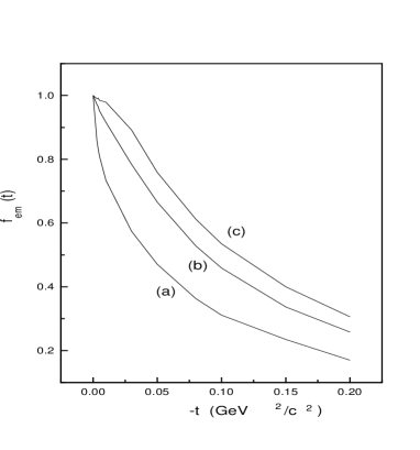
The dependence of the shape on the ratio $\rho$ is illustrated by the plots of the pion form factor in Fig.1.

Refer to caption
Figure 1: Plots of the pion electromagnetic form factor for the following values of the parameters: $\alpha=0.3~{}M_{\pi}$; (a) $\beta$=0.02 GeV; (b) $\beta$=0.04 GeV; (c) $\beta$=0.06 GeV.

For the comparison with the experimental data we shall retain however only the cases with $\rho\geq 1$, which fit the expected growth of the form factor at time-like $t$ and are also in agreement with our initial assumption $Q^{2}>0$.

The quark masses used in the calculations have been determined together with the cut-off parameter $\alpha$ from the fit of the decay constants of pseudoscalar mesons [10]. We take: $m_{u}=7$MeV, $m_{d}=$10MeV, $m_{s}$= 400MeV and $\alpha=0.3~{}M$, which give $F_{\pi}:F_{K}:F_{D}:F_{B}:F_{D_{s}}=130.:160:254:144:386.$, in agreement with the experimental data. We note that the values of the quark masses are rather close to the values suggested by chiral symmetry scheme [11].

Moreover, by using the normalization condition (12) we get in the charged pion case $T_{0}\approx 10^{-22}$s, which is in agreement with the low values for the quark masses we used.

Taking now $\rho\approx 1.(\beta=0.04$ GeV in the pion case), we find the following values for the charge radii: $r_{\pi^{\pm}}^{2}=1.6$ fm2, $r_{K^{\pm}}^{2}$=1.0 fm2, $r_{K^{0}}$=-0.17 fm2, which are much larger than the measured ones: $r_{\pi^{\pm}}$=0.44 fm2, $r_{K^{\pm}}$=0.29 fm2, $r_{K^{0}}$=-0.054 fm2 [12]. We notice, however, the negative sign of $r_{K^{0}}^{2}$ in agreement with the experimental result.This shows that the contribution of the heavy quark is dominant.

The values we obtained for the charge radii suggest that the approximation (19) is inadequate. A simple way to improve it is to replace the symmetry scheme based on the full Lorentz group with the symmetry under the collinear group which is equivalent with the flux tube model with frozen transverse degrees [13]. The longitudinal and the temporal degrees of freedom are then the only active and the multiple integral in eq.(S0.Ex14) reduces to a simple one. By using less drastic cuts of the internal momenta we expect to obtain a slower decrease of the form factors and a better agreement with the experimental data. The work on this line is in progress.


Acknowledgements

The author thanks Prof. H. Leutwyler for the kind hospitality at the Institute of Theoretical Physics of the University of Bern. This work was completed during author’s visit at ITP-Bern, which has been supported by the Swiss National Science Foundation under Contract No. 7 IP 051219. The partial support of the Romanian Academy through the Grant No. 329/1997 is also acknowledged.

References

  • [1] E. E. Salpeter and H. A. Bethe Phys. Rev. 84 (1951) 1232; M. Gell-Mann and F. Low, Phys. Rev. 84 (1951) 350; N. Nakanishi, Prog. Theor. Phys. Suppl. 43 (1969) 1.
  • [2] M. Neubert, Phys. Rep. 245 (1994) 259.
  • [3] R. C. Brower, M. B. Gavela, R. Gupta and G. Maturana, Phys. Rev. Lett. 53 (1984) 1318; N. Cabibbo, G. Martinelli and R. Petronzio Nucl. Phys. B 244 (1984) 381.
  • [4] J. Gasser and H. Leutwyler, Nucl. Phys. B 250 (1985) 465; 517; 539.
  • [5] B. Grinstein, M. B. Wise and N. Isgur, Phys. Rev. Lett. 56 (1986) 298; N. Isgur, D. Scora, B. Grinstein and M. B. Wise, Phys. Rev. D 39 (1989) 799.
  • [6] R. N. Faustov, Ann. Phys. (N.Y.) 78 (1973) 176.
  • [7] M. Wirbel, B. Stech and M. Bauer, Z. Phys. C 29 (1985) 637.
  • [8] P. L. Chung, F. Coester and W. N. Polizou, Phys. Lett. B 205 (1988) 545; W. Jaus, Phys. Rev. D 41 (1990) 3394.
  • [9] H. Leutwyler, Ann. Phys. (N.Y.) 235 (1994) 165.
  • [10] L. Micu, Phys. Rev. D 55 (1997) 4151.
  • [11] H. Leutwyler, Phys. Lett. B378 (1996) 313.
  • [12] S. R. Amendolia et al. (NA7 coll.) Nucl. Phys. B277 (1986) 168; W. R. Molzen et al. Phys. Rev. Lett. 41 (1978) 1213.
  • [13] M. Burkhardt, Phys. Rev. D 56 (1997) 7501.