Abstract

We introduce an efficient configuration space technique which allows one to compute a class of Feynman diagrams which generalize the scalar sunset topology to any number of massive internal lines. General tensor vertex structures and modifications of the propagators due to particle emission with vanishing momenta can be included with only a little change of the basic technique described for the scalar case. We discuss applications to the computation of $n$-body phase space in $D$-dimensional space-time. Substantial simplifications occur for odd space-time dimensions where the final results can be expressed in closed form through elementary functions. We present explicit analytical formulas for three-dimensional space-time.

1 Introduction

Up to now one has not been able to observe any contradictions to the predictions of the Standard Model of particle interactions. Possible deviations from the Standard Model or revelations of new physics are expected to be quite small at the energies of present accelerators. Future experiments focus on tests of the Standard Model with an unprecedented precision [1, 2]. The present accuracy of experimental data already demands new levels of accuracy in the theoretical predictions of perturbation theory [3]. This requirement leads to the necessity to compute multiloop Feynman diagrams beyond the one-loop level (as a review, see e.g. [4]). Within the Standard Model the diagrams of perturbation theory may contain a multitude of internal and external lines with different particles and different masses that makes the task of evaluation of such diagrams rather complicated already at the two-loop level. The computation of different subsets of diagrams in different regimes of their masses and their external momenta is now an active field of research and often requires extensive use of direct numerical methods [5].

(a)(b)

(c)(d)

Figure 1: (a) a sunset diagram with three different masses $m_{1}$, $m_{2}$ and $m_{3}$ (b) general topology of the class of water melon diagrams (c) one half of a cut $n=6$ water melon diagram in the Standard Model representing the spectral function for the process $q\rightarrow q\ell\bar{\nu}_{\ell}gZH$ (d) an example of a water melon diagram with multiple gluon radiation from internal lines

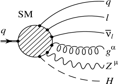
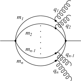
Among the many two-loop topologies the two-loop sunset diagrams with different values of internal masses as shown in Fig. 1(a) have been recently studied in some detail (see e.g. [6, 7, 8, 9, 10, 11] and references therein). In the present note we describe an efficient method for computing and investigating a class of diagrams that generalizes the sunset topology to any number of internal lines (massive propagators) in arbitrary number of space-time dimensions. We call the class of diagrams with this topology water melon diagrams. Fig. 1(b) shows a diagram with water melon topology. In our opinion, the method presented in the paper completely solves the problem of computing this class of diagrams. The method is simple and reduces the multiloop calculation of a water melon diagram to a one-dimensional integral which includes only well known special functions in the integrand for any values of internal masses. The technique is universal and requires only minor technical modifications for additional tensor structure of vertices or internal lines (propagators), i.e. tensor particles or/and fermions can be added at no extra cost. The method can also handle form factor type processes at small momentum transfer – the inclusion of lines of incoming/outgoing particles with vanishing momenta and derivatives thereof with respect to their momenta is straightforward and is done within the same calculational framework. Our final one-dimensional integral representation for water melon diagrams is well suited for any kind of asymptotic estimates in masses and/or momentum. The principal aim of our paper is to work out a practical tool for computing water melon diagrams. In the Euclidean domain the numerical procedures derived from our representation are efficient and reliable, i.e. stable against error accumulation. The most interesting part of our analysis of water melon diagrams is the construction of the spectral decomposition of water melon diagrams, i.e. we determine the discontinuity across the physical cut in the complex plane of squared momentum. We suggest a novel technique for the direct construction of the spectral density of water melon diagrams which is based on an integral transform in configuration space. We compare our approach to the more traditional way of computing the spectral density where one uses an analytic continuation in momentum space. Because the analytic structure of water melon diagrams is completely fixed by the dispersion representation, our attention is focussed on the computation of the spectral density as the basic quantity important both for applications and the theoretical investigation of the diagram. The complete polarization function can then be easily reconstructed from the spectral density with the help of dispersion relations. In addition we derive some useful formulas for the polarization function in the Euclidean domain and present explicit results for some limiting cases where analytical formulas can be found.

The paper is organized as follows. In the beginning of Sec. 2 we describe some general properties of water melon diagrams and fix our notation. In Sec. 2.1 we introduce the configuration space representation of water melon diagrams. In Sec. 2.2 we discuss the ultraviolet (UV) divergence structure of water melon diagrams and present the way to regularize the UV divergences by subtraction. In Sec. 2.3 some previously known results are reproduced using our configuration space techniques. Sec. 2.4 contains explicit examples in odd-dimensional space-time. In Sec. 2.5 we discuss expansions in masses and/or momenta in the Euclidean domain. In Sec. 3 we consider the computation of the spectral density of water melon diagrams by analytic continuation in momentum space. Sec. 4 is devoted to the direct computation of the spectral density of water melon diagrams without taking recourse to Fourier transforms. Sec. 5 gives our conclusions.

2 The general framework

Sunset-type diagrams are two-point functions with $n$ internal propagators connecting the initial and final vertex. The sunset diagram shown in Fig. 1(a) is the leading order perturbative correction to the lowest order propagator in $\phi^{4}$-theory, i.e. it is a two-point two-loop diagram with three internal lines. The corresponding leading order perturbative correction in $\phi^{3}$-theory is a one-loop diagram and can be considered as a degenerate case of the prior example. A straightforward generalization of this topology is a correction to the free propagator in $\phi^{n+2}$-theory that contains $n$ loops and $(n+1)$ internal lines (see Fig. 1(b)). We call them water melon diagrams. In a general field theory the internal lines may have different masses and may carry different Lorenz structures or may contain space-time derivatives. An example of the latter situation is a leading quantum correction in higher orders of Chiral Perturbation Theory for pseudoscalar mesons where the vertices contain multiple derivatives of the meson fields. In order to accommodate such general structures we represent a general water melon diagram as a correlator of two monomials $j_{n}(x)$ of the form

$$j_{n}(x)={\cal D}_{\mu_{1}}\phi_{1}\cdots{\cal D}_{\mu_{n}}\phi_{n}$$ (1)

where the fields $\phi_{n}$ have masses $m_{n}$ and where ${\cal D}_{\mu}$ is a derivative with multi-index $\mu=\{\mu_{1},\ldots,\mu_{k}\}$ standing for ${\cal D}_{\mu}=\partial^{k}/\partial x_{\mu_{1}}\ldots\partial x_{\mu_{k}}$. The water melon diagrams are contained in the leading order expression for the polarization function

$$\Pi(x)=\langle Tj_{n}(x)j_{n^{\prime}}(0)\rangle$$ (2)

which is explicitly given by a product of propagators and/or their derivatives,

$$\Pi(x)={\cal D}_{\mu_{1}\nu_{1}}(x,m_{1})\cdots{\cal D}_{\mu_{n}\nu_{n}}(x,m_{n}).$$ (3)

Here ${\cal D}_{\mu\nu}(x,m)={\cal D}_{\mu}{\cal D}_{\nu}D(x,m)$ is a derivative of the propagator $D(x,m)$ with respect to the coordinate $x$ with a pair of multi-indices $\{\mu,\nu\}$. The propagator $D(x,m)$ of a massive particle with mass $m$ in $D$-dimensional (Euclidean) space-time is given by

$$D(x,m)=\frac{1}{(2\pi)^{D}}\int\frac{e^{ip_{\mu}x^{\mu}}d^{D}p}{p^{2}+m^{2}}=\frac{(mx)^{\lambda}K_{\lambda}(mx)}{(2\pi)^{\lambda+1}x^{2\lambda}}$$ (4)

where we write $D=2\lambda+2$. $K_{\lambda}(z)$ is a McDonald function (a modified Bessel function of the third kind, see e.g. [12]). The propagator $D(x,m)$ depends only on the length of the space-time vector $|x|=\sqrt{x_{\mu}x^{\mu}}$ for which we simply write $x$. We consider only the case $n=n^{\prime}$ (equal number of lines at the initial and final vertex). We thus exclude tadpole configurations (the leaves of this water melon) which add nothing interesting. Taking the limit $m\rightarrow 0$ in Eq. (4) we get an explicit form of the massless propagator

$$D(x,0)=\frac{1}{(2\pi)^{D}}\int\frac{e^{ip_{\mu}x^{\mu}}d^{D}p}{p^{2}}=\frac{\Gamma(\lambda)}{4\pi^{\lambda+1}x^{2\lambda}}$$ (5)

where $\Gamma(\lambda)$ is the Euler $\Gamma$-function. Note that propagators of particles with nonzero spin in configuration space representation can be obtained from the scalar propagator by differentiation with respect to the space-time point $x$. This does not change the functional $x$-structure and causes only minor modification of the basic technique. For instance, the propagator for the fermion (spin 1/2 particle) is given by

$$S(x,m)=(i\gamma_{\mu}\frac{\partial}{\partial x_{\mu}}+m)D(x,m)$$ (6)

with $\gamma_{\mu}$ is a Dirac matrix.

The next generalization consists in extending our configuration space description to the case of particle radiation from internal lines. The modification of the internal line with mass $m$ due to the emission of a particle with momentum $q$ at the vertex $V(p,q)$ reads

$$D(p,m) = {1\over p^{2}+m^{2}}\rightarrow{1\over p^{2}+m^{2}}V(p,q){1\over(p-q)^{2}+m^{2}}$$ (7)

$$\buildrel q=0\over{=} {1\over p^{2}+m^{2}}V(p,0){1\over p^{2}+m^{2}}=-V(p,0){d\over dm^{2}}{1\over p^{2}+m^{2}}.$$

The functional $x$-space structure of the corresponding internal line is not changed by this modification. Therefore such contributions can be obtained either by differentiating the original water melon diagram without particle emission with respect to the mass $m$ or by direct differentiation of the propagator which leads to a change of the index of the corresponding McDonald function. The explicit representation for the modified internal line with mass $m$ is given by

$$\frac{1}{(2\pi)^{D}}\int\frac{e^{ip_{\nu}x^{\nu}}d^{D}p}{(p^{2}+m^{2})^{\mu+1}}=\frac{1}{(2\pi)^{\lambda+1}2^{\mu}\Gamma(\mu+1)}{\left(\frac{m}{x}\right)^{\lambda-\mu}K_{\lambda-\mu}(mx)}.$$ (8)

This modified propagator is a product of some power of $x$ and the McDonald function as in the standard propagator shown in Eq. (4). The only difference is in the index $(\lambda-\mu)$ of the McDonald function which is inessential for applications. This does not change the general functional structure of the representation constructed below. If there is only one-particle emission, the form factor type diagrams with any number of massive internal lines can be obtained for any value of $q$ in a closed form. One encounters such diagrams when analyzing baryon transitions within perturbation theory. The corresponding formulas will be discussed elsewhere. Also the change of the mass along the line in Eq. (7) is allowed for vanishing incoming/outgoing particle momenta which allows for the possibility to discuss processes with radiation of gauge bosons such as $b\rightarrow s\gamma$ transition for baryons within the sum rules approach. As described above, such generalizations can easily be accommodated in our approach without any change in the basic framework. From now on we therefore mostly concentrate on the basic scalar master configuration of the water melon diagram which contains all features necessary for our discussion.

Eq. (3) contains all information about the water melon diagrams and in this sense is the final result for the class of diagrams under consideration. Of some particular interest is the spectral decomposition of the polarization function $\Pi(x)$ which is connected to the particle content of a model. As a particular example one can consider a water melon diagram with a vertex connecting various particles of the Standard Model as shown in Fig. 1(c). The knowledge of the analytic structure of the propagators $D(x,m)$ entering Eq. (3) is sufficient for determining the analytic structure of the polarization function $\Pi(x)$ itself. For applications, however, one may need the Fourier transform of the polarization function $\Pi(x)$ given by

$$\tilde{\Pi}(p)=\int\Pi(x)e^{ip_{\mu}x^{\mu}}dx=\int\langle Tj_{n}(x)j_{n^{\prime}}(0)\rangle e^{ip_{\mu}x^{\mu}}dx.$$ (9)

The tilde “$\sim$” on the Fourier transform $\tilde{\Pi}(p)$ will be dropped in the following. The computation of an explicit expression for the Fourier transform $\Pi(p)$ for three-line (or two-loop) water melon diagrams (the genuine sunset diagram) is described in a number of papers in the literature. In the standard, or momentum, representation the quantity $\Pi(p)$ is calculated from a $(n-1)$-loop diagram with $(n-1)$ integrations over the entangled loop momenta which makes the computation difficult when the number of internal lines becomes large. Our technique consists in computing the integral in Eq. (9) directly using the product of propagators Eq. (3) with their explicit form given by Eq. (4). The key simplifying observation is that the rotational invariance of the expression in Eq. (3) allows one to perform the angular integrations explicitly. As a result one is left with a one-dimensional integral over the radial variable in Eq. (9). The remaining integrand has a rather simple structure in the form of a product of Bessel functions and powers of $x$ which is a convenient starting point for further analytical or numerical processing.

2.1 Configuration space representation

In the present paper we focus on the technical simplicity and the practical applicability of the configuration space approach to the computation of water melon diagrams as written down in Eqs. (3), (4) and (9). The idea of exploiting $x$-space techniques for the calculation of Feynman diagrams has a long history. Configuration space techniques were successfully used for the evaluation of massless diagrams with quite general topologies in [13] and marked a real breakthrough in multiloop computations before the invention of the integration-by-parts technique.

The case of massive diagrams for general topologies was considered in some detail in [14] with $x$-space integration techniques. As it turns out, the $x$-space technique has not been very successful for general many-loop massive diagrams. The angular integrations do not decouple and no decisive simplification occurs. It is the special topology of water melon diagrams which makes the $x$-space technique so efficient. Using $x$-space techniques one can completely solve the problem of computing this class of diagrams.

So, let us taste the water melon. The angular integration in Eq. (9) can be explicitly done in $D$-dimensional space-time with the result

$$\int d^{D}\hat{x}e^{ip_{\mu}x^{\mu}}=2\pi^{\lambda+1}\left(\frac{px}{2}\right)^{-\lambda}J_{\lambda}(px)$$ (10)

where $p=|p|$, $x=|x|$. $J_{\lambda}(z)$ is the usual Bessel function and $d^{D}\hat{x}$ is the rotationally invariant measure on the unit sphere in the $D$-dimensional (Euclidean) space-time. The generalization of Eq. (10) to more complicated integrands with additional tensor structure $x^{\mu_{1}}\cdots x^{\mu_{k}}$ is straightforward and merely leads to different orders of the Bessel function after angular averaging. The corresponding order of the Bessel function can be easily inferred from the expansion of the plane wave function $\exp(ip_{\mu}x^{\mu})$ in a series of Gegenbauer polynomials $C^{\lambda}_{j}(p_{\mu}x^{\mu}/px)$. The Gegenbauer polynomials are orthogonal on a $D$-dimensional unit sphere, and the expansion of the plane wave $\exp(ip_{\mu}x^{\mu})$ reads

$$\exp(ip_{\mu}x^{\mu})=\Gamma(\lambda)\left(\frac{px}{2}\right)^{-\lambda}\sum_{l=0}^{\infty}i^{l}(\lambda+l)J_{\lambda+l}(px)C^{\lambda}_{l}(p_{\mu}x^{\mu}/px).$$ (11)

This formula allows one to single out an irreducible tensorial structure from the angular integration in the Fourier integral in Eq. (9). Integration techniques involving Gegenbauer polynomials for the computation of massless diagrams are described in detail in [13] where many useful relations can be found (see also [15]). Our final representation of the Fourier transform of a water melon diagram is given by the one-dimensional integral

$$\Pi(p)=2\pi^{\lambda+1}\int_{0}^{\infty}\left(\frac{px}{2}\right)^{-\lambda}J_{\lambda}(px)D(x,m_{1})\cdots D(x,m_{n})x^{2\lambda+1}dx$$ (12)

which is a special kind of integral transformation with a Bessel function as a kernel. This integral transformation is known as the Hankel transform. The representation given by Eq. (12) is quite universal regardless of whether tensor structures are added or particles with vanishing momenta are radiated from any of the internal lines. An example of a water melon diagram with internal gluon emission is shown in Fig. 1(d).

Next we discuss the analytic structure of a water melon diagram in the complex $p$-plane and also the behaviour of $\Pi(p)$ near threshold. From Eq. (12) it is clear that $\Pi(p)$ is analytic in the strip $|{\rm Im}(p)|<M=\sum_{i=1}^{n}m_{i}$. In terms of the relativistically invariant variable $p^{2}$ this means that the function $\Pi(p^{2})$ is analytic for ${\rm Re}(p^{2})>-M^{2}$ implying that the function $\Pi(p)$ becomes singular at the energy $E=M$ in the Minkowskian region. Depending on the number of internal lines in the diagram this singularity is either a pole for the most degenerate case of only one single propagator or a cut in the case of several propagators.

2.2 Regularization and subtraction

The general formula for the Fourier transform (12) allows for an explicit numerical computation for any momentum $p$ in the Euclidean domain. However, if $D>2$ and the number of propagators is sufficiently large, the integral diverges in the ultraviolet (UV) region or, equivalently, at small $x$. Note that for $D=2$ there are only logarithmic singularities at the origin ($\lambda=0$ for the propagator Eq. (4)) which makes this case technically simpler. Also for $D=2$ the strength of the singularity does not increase with the number of internal lines as dramatically as for higher dimensions. In the general case the UV divergence prevents one from taking the limit $D\rightarrow D_{0}$ where $D_{0}$ is an integer number of physical space-time dimensions. Taken by itself, the representation given by Eq. (12) determines the dimensionally regularized function for complex space-time dimension $D$. For the scalar propagator in space-time with $D_{0}=4$ the singularity at small $x$ is given by $x^{-2}$. For explicit computations in this paper we normally use dimensional regularization, although our particular way of regularization is not always the orthodox one. The structure of the UV divergence is very simple for the general water melon diagram. Any water melon diagram only has an overall divergence without subdivergences if the $R$-operation using normal ordering and vanishing tadpoles (see e.g. [16]) is properly defined which means that the water melon is stripped off its leaves. Thus the renormalization of water melon diagrams in the representation given by Eq. (12) is simple and well suited for a numerical treatment which is important for practical applications.

Besides dimensional regularization the momentum space subtraction technique is sometimes used for dealing with UV divergences. Its implementation is very simple in the representation given by Eq. (12). Subtractions at the origin $p=0$ are always possible as long as one has massive internal lines which prevent the appearance of infrared singularities. If this is the case, the subtraction amounts to expanding the function

$$\left(\frac{px}{2}\right)^{-\lambda}J_{\lambda}(px),$$ (13)

(which is a kernel or weight function of the integral transformation in Eq. (12)) in a Taylor series around $p=0$ in terms of a polynomial series in $p^{2}$. The order $N$ subtraction is achieved by writing

$$\left[\left(\frac{px}{2}\right)^{-\lambda}J_{\lambda}(px)\right]_{N}=\left(\frac{px}{2}\right)^{-\lambda}J_{\lambda}(px)-\sum_{k=0}^{N}\frac{(-1)^{k}}{k!\Gamma(\lambda+k+1)}\left(\frac{px}{2}\right)^{2k}$$ (14)

and by keeping $N$ terms in the expansion on the right hand side. Substituting expansion Eq. (14) into expression (12) leads to a momentum subtracted polarization function

$$\Pi_{\rm Mom}(p)=\Pi(p)-\sum_{k=0}^{N}\frac{p^{2k}}{k!}\left(\frac{d}{dp^{2}}\right)^{k}\Pi(p)|_{p^{2}=0}$$ (15)

which is finite if the number of subtractions is sufficiently high. The function $\Pi(p)$ itself is divergent as well as any derivative on the right hand side of Eq. (15) and requires regularization. However, the difference or the quantity $\Pi_{\rm Mom}(p)$ is finite and independent of any regularization used to give a meaning to the individual terms in Eq. (15). Note that the expansion (14) is a polynomial in $p^{2}$ in accordance with the general structure of the $R$-operation [16]. The number $N$ of necessary subtractions is determined by the divergence index of the diagram and can be found according to the standard rules [16]. The subtraction at the origin $p=0$ is allowed if there is at least one massive line in the diagram and an arbitrary number of massless lines. If there are no massive internal lines, the corresponding diagram can easily be calculated analytically and the problem of subtraction is trivial. After having performed the requisite subtraction one can take the limit $D\rightarrow D_{0}$ in Eq. (12) where $D_{0}$ is an integer. The diagram as a whole becomes finite after the subtraction. In order to obtain a deeper insight and for reasons of technical convenience it is useful to give a meaning to every individual term in the expansion in Eq. (12) after substituting the difference given by Eq. (14) which will then finally lead to Eq. (15). To make the individual terms meaningful one has to introduce an intermediate regularization. This intermediate regularization can in principle be the standard dimensional regularization. However, the regularization in this particular case can be also achieved by adding a factor $x^{2\omega}$ to the integration measure which, in practice, turns into $(\mu x)^{2\omega}$ in order to keep the overall dimensionality of the diagram correct, where $\mu$ is an arbitrary mass parameter. Thus, all propagators are taken in the form of an integer number of dimensions (depending on the choice of the space-time) but the integration measure is modified to provide regularization. We refer to this procedure of auxiliary regularization as an unorthodox dimensional regularization [17]. Note that similar modifications of dimensional regularization are known in other applications. For instance, in some supersymmetric theories one has to keep the four dimensional structure of tensor fields to preserve the Ward identities for the regularized theory. The corresponding modification of the standard dimensional regularization is then called dimensional regularization by dimension reduction.

Let us now demonstrate that finite quantities (like the momentum subtracted polarization operator in Eq. (15)) are independent of the intermediate regularization scheme used. Consider the simplest case of one massive and one massless line. The corresponding diagram requires only one subtraction according to the standard power counting by noting that its divergence index is equal to zero. Within ordinary dimensional regularization the polarization function reads

$$\Pi^{D}(p) = \int D(x,m)D(x,0)e^{ip_{\mu}x^{\mu}}d^{D}x$$ (16)

$$= {\Gamma(1-\lambda)m^{2\lambda-2}\over(4\pi)^{\lambda+1}\lambda}\,{}_{2}F_{1}\left(1,1-\lambda;\lambda+1;-\frac{p^{2}}{m^{2}}\right)$$

where ${}_{2}F_{1}(a,b;c;z)$ is a hypergeometric function and $\lambda=1-\varepsilon$. Within the unorthodox dimensional regularization we find

$$\Pi_{4,\omega}(p) = \int D_{4}(x,m)D_{4}(x,0)e^{ip_{\mu}x^{\mu}}x^{2\omega}d^{4}x$$ (17)

$$= \frac{\Gamma(1+\omega)\Gamma(\omega)(m^{2}/4)^{-\omega}}{(4\pi)^{2}}\,{}_{2}F_{1}\left(1+\omega,\omega;2;-\frac{p^{2}}{m^{2}}\right).$$

It is straightforward to see that in the limits $\omega\rightarrow 0$ and $\varepsilon\rightarrow 0$ both $\Pi^{D}(p)-\Pi^{D}(0)$ and $\Pi_{4,\omega}(p)-\Pi_{4,\omega}(0)$ are finite and equal to each other in accordance with Eq. (15) and general statements of the $R$-operation.

The unorthodox dimensional regularization scheme is only an intermediate step in the calculation of finite quantities. However, in some cases it may lead to dramatic simplifications in the calculation of the relevant integrals. As we shall see later on, the computation of the limit $D\rightarrow D_{0}=3$ (and of any odd-dimensional space-time) can be explicitly done for any water melon diagram within unorthodox dimensional regularization because of the simple form of the propagators and the weight function: they contain the exponential functions instead of Bessel functions. The use of ordinary dimensional regularization would require the full computation for the noninteger space-time dimension $D$ first which is not possible for an arbitrary diagram.

2.3 Test of the technique with known results

In this subsection we reproduce some known results with our configuration space techniques. The complexity of the examples increases with the number of massive propagators occuring in the water melon diagram. The completely massless case is quite trivial and will not be discussed futher. Water melon diagrams with one massive line and an arbitrary number of massless lines are solved with the formula

$$\int_{0}^{\infty}x^{\mu}K_{\nu}(mx)dx=2^{\mu-1}m^{-\mu-1}\Gamma\left(\frac{1+\mu+\nu}{2}\right)\Gamma\left(\frac{1+\mu-\nu}{2}\right)$$ (18)

which allows one to compute all necessary counterterms. Water melon diagrams containing two massive lines and arbitrary number of massless lines are also solved in a closed analytical form with the formula

$$\int_{0}^{\infty}x^{2\alpha-1}K_{\mu}(mx)K_{\mu}(mx)dx={2^{2\alpha-3}\over m^{2\alpha}\Gamma(2\alpha)}\Gamma(\alpha+\mu)\Gamma(\alpha)\Gamma(\alpha)\Gamma(\alpha-\mu).$$ (19)

There exists a generalization of Eq. (19) to different masses and indices of the McDonald functions as well. We do not dwell upon this point here. As a simple example we give the result for a three-loop water melon diagram with two massive and two massless lines at vanishing external momentum. The analytical expression for the diagram in the configuration space representation is

$$\Pi(0)=\int D(x,m)^{2}D(x,0)^{2}d^{D}x=\int\left(\frac{(mx)^{\lambda}K_{\lambda}(mx)}{(2\pi)^{\lambda+1}x^{2\lambda}}\right)^{2}\left(\frac{\Gamma(\lambda)}{4\pi^{\lambda+1}x^{2\lambda}}\right)^{2}d^{D}x.$$ (20)

While the angular integration in $D$-dimensional space-time is trivial the problem of residual radial integration is solved by Eq. (19). The result for the integral in Eq. (20) is

$$\Pi(0)=\left(\frac{m^{2}}{4}\right)^{3\lambda-1}\frac{1}{2^{8}\pi^{3\lambda+3}}\frac{\Gamma(\lambda)^{2}\Gamma(1-\lambda)\Gamma(1-2\lambda)^{2}\Gamma(1-3\lambda)}{\Gamma(\lambda+1)\Gamma(2-4\lambda)}.$$ (21)

This result corresponds to the quantity $M_{1}$ which is the simplest basis element for the computation of massive three-loop diagrams in a general three-loop topology considered in [18].

Next we turn to a sunset diagram with three massive lines, i.e. the two-loop water melon diagram. There is an analytical expression for such a diagram at some special values of external momenta computed within dimensional regularization [10]. We reproduce this result here. We start with Eq. (9) setting $n=n^{\prime}=3$. The angular integration just gives the volume of $D$-dimensional sphere. We then arrive at Eq. (12) with $n=3$. Therefore the one-dimensional integral to analyze is

$$\Pi_{D}(p)=2\pi^{\lambda+1}\int_{0}^{\infty}\left(\frac{px}{2}\right)^{-\lambda}J_{\lambda}(px)D(x,m_{1})D(x,m_{2})D(x,m_{3})x^{2\lambda+1}dx.$$ (22)

To localize the finite part we first use momentum subtraction and separate $\Pi_{D}(p)$ into its finite and infinite (but dimensionally regularized) parts

$$\Pi_{D}(p)=\Pi_{\rm Mom}(p)+\Pi_{\rm sing}(p)$$ (23)

where $\Pi_{\rm Mom}(p)$ is a momentum subtracted polarization function and $\Pi_{\rm sing}(p)$ is a counterterm in dimensional regularization. Only two subtractions are necessary by power counting. The explicit expression for the momentum subtracted polarization function is

$$\Pi_{\rm Mom}(p) = 2\pi^{\lambda+1}\int_{0}^{\infty}\left[\left(\frac{px}{2}\right)^{-\lambda}J_{\lambda}(px)\right]_{1}D(x,m_{1})D(x,m_{2})D(x,m_{3})x^{2\lambda+1}dx$$ (24)

$$= 2\pi^{\lambda+1}\int_{0}^{\infty}\left[\left(\frac{px}{2}\right)^{-\lambda}J_{\lambda}(px)-\frac{1}{\Gamma(\lambda+1)}+\frac{p^{2}x^{2}}{4}\frac{1}{\Gamma(\lambda+2)}\right]$$

$$\qquad\times D(x,m_{1})D(x,m_{2})D(x,m_{3})x^{2\lambda+1}dx.$$

The singular part is given by a first order polynomial in $p^{2}$ with coefficients $A$, $B$ whose values depend on the regularization scheme (in this case dimensional regularization is used)

$$\Pi_{\rm sing}(p) = A+p^{2}B$$ (25)

$$= \frac{2\pi^{\lambda+1}}{\Gamma(\lambda+1)}\int_{0}^{\infty}D(x,m_{1})D(x,m_{2})D(x,m_{3})x^{2\lambda+1}dx$$

$$-p^{2}\frac{2\pi^{\lambda+1}}{4\Gamma(\lambda+2)}\int_{0}^{\infty}x^{2}D(x,m_{1})D(x,m_{2})D(x,m_{3})x^{2\lambda+1}dx.$$

With this representation our strategy applies straightforwardly. In the momentum subtracted part one can forego the regularization (it is finite by $R$-operation) and perform the one-dimensional integration numerically for $D=4$. The counterterms are then simple numbers independent of $p$. They contain divergent parts (regularized within dimensional regularization) and need to be computed only once to recover the function $\Pi(p)$ for any $p$.

In the particular case of the sunset diagram (three lines) the necessary integrals are known analytically in their full form and can be found in integral tables (e.g. [19]). Using the tables may not always be convenient and we therefore present a simplified approach which allows one to deal even with the complicated cases in a simpler manner. Let us specify to the particular case $p=m_{1}+m_{2}-m_{3}$ (pseudothreshold) where an analytical answer exists [10]. For simplicity we choose $m_{1}=m_{2}=m_{3}/2=m$. Then $p=0$ and $\Pi_{\rm Mom}(0)=0$ (this is a regular function at this Euclidean point). In this case the counterterm $p^{2}B$ vanishes because at finite $\varepsilon$ the quantity $B$ is finite. We thus only have to consider $A$. On the other hand our considerations are completely general since one only requires more terms in the $p^{2}$-expansion for arbitrary $p$. For the special mass configuration considered here the result of [10] reads

$$\Pi_{D}^{ref}(0)=\pi^{4-2\varepsilon}\frac{m^{2-4\varepsilon}\Gamma^{2}(1+\varepsilon)}{(1-\varepsilon)(1-2\varepsilon)}\left[-\frac{3}{\varepsilon^{2}}+\frac{8\ln 2}{\varepsilon}-8\ln^{2}2\right]+O(\varepsilon).$$ (26)

This result can be extracted from the first line of Eq. (25) using the integral tables given in [19]. However, in the general mass caes the necessary formulas are rather cumbersome. Even for the special mass configuration considered here they are not so simple. We therefore discuss a short cut which allows one to obtain results immediately without having to resort to integral tables. What we really only need is an expansion in $\varepsilon$. Basically we need the integral

$$\int_{0}^{\infty}D(x,m)D(x,m)D(x,2m)x^{2\lambda+1}dx$$ (27)

which is of the general form

$$\int_{0}^{\infty}x^{\rho}K_{\mu}(mx)K_{\mu}(mx)K_{\mu}(2mx)dx$$ (28)

($\mu=\lambda$ and $\rho=1-\lambda$ in our case). For two McDonald functions in the integrand (without the last one in the above equation, for instance) the result is given by Eq. (19). Let us reduce the problem at hand to Eq. (19) and do our numerical evaluations with functions in four-dimensional space-time where no regularization is necessary. To do this we subtract the leading singularities at small $\xi$ from the last McDonald function in Eq. (28) using the series expansion near the origin,

$$\left(\frac{\xi}{2}\right)^{\lambda}K_{\lambda}(\xi)=\frac{\Gamma(\lambda)}{2}\left[1+\frac{1}{1-\lambda}\left(\frac{\xi}{2}\right)^{2}-\frac{\Gamma(1-\lambda)}{\Gamma(1+\lambda)}\left(\frac{\xi}{2}\right)^{2\lambda}\right]+O(\xi^{4},\xi^{2+2\lambda}).$$ (29)

After decomposing the whole answer into finite and singular parts as $(2\pi)^{2D}A=F+S$ (where the total normalization of [10] has been adopted in the definition of $F$ and $S$) we find for the singular part

$$S\ =\ \frac{(2\pi)^{D}m^{2\lambda}}{\Gamma(\lambda+1)}\int_{0}^{\infty}x^{2(1-\lambda)-1}K_{\lambda}(mx)K_{\lambda}(mx)$$ (30)

$$\times\frac{\Gamma(\lambda)}{2}\left[1+\frac{(mx)^{2}}{1-\lambda}-\frac{\Gamma(1-\lambda)}{\Gamma(1+\lambda)}(mx)^{2\lambda}\right]dx$$

$$= \frac{(2\pi)^{D}m^{2-4\varepsilon}}{\Gamma(\lambda+1)}\int_{0}^{\infty}\xi^{2\varepsilon-1}K_{\lambda}(\xi)K_{\lambda}(\xi)\frac{\Gamma(\lambda)}{2}\left[1+\frac{\xi^{2}}{1-\lambda}-\frac{\Gamma(1-\lambda)}{\Gamma(1+\lambda)}\xi^{2\lambda}\right]d\xi$$

$$= \pi^{4-2\varepsilon}\frac{m^{2-4\varepsilon}\Gamma^{2}(1+\varepsilon)}{(1-\varepsilon)(1-2\varepsilon)}\left[-\frac{3}{\varepsilon^{2}}+\frac{8\ln 2}{\varepsilon}+8(2-2\ln 2-\ln^{2}2)\right]+O(\varepsilon).$$

The pole contributions coincide with the result in Eq. (26) while the finite part is different. It is corrected by the finite expression

$$F = \frac{(2\pi)^{D}m^{2\lambda}}{\Gamma(\lambda+1)}\int_{0}^{\infty}x^{2(1-\lambda)-1}K_{\lambda}(mx)K_{\lambda}(mx)$$

$$\times\left\{(mx)^{\lambda}K_{\lambda}(2mx)-\frac{\Gamma(\lambda)}{2}\left[1+\frac{(mx)^{2}}{1-\lambda}-\frac{\Gamma(1-\lambda)}{\Gamma(1+\lambda)}(mx)^{2\lambda}\right]\right\}dx.$$

Because this quantity is finite (no strong singularity at small $x$) one can put $D=4$ to get

$$F=16\pi^{4}m^{2}\int_{0}^{\infty}\frac{dx}{x}K_{1}(x)K_{1}(x)\left\{xK_{1}(2x)-\frac{1}{2}\left[1+x^{2}(-1+2\gamma_{E}+2\ln x)\right]\right\}$$ (32)

where $\gamma_{E}$ is the Euler’s constant gamma with the numerical value $0.577\ldots$. The numerical integration results in

$$F=16\pi^{4}m^{2}[-0.306853\ldots\ ]=16\pi^{4}m^{2}[-(1-\ln 2)\times 1.0000\ldots\ ].$$ (33)

Now one can restore all $\varepsilon$ dependence in the normalization factors as in Eqs. (26) and (30) because $F$ is not singular in $\varepsilon$ and this change of normalization is absorbed in the $O(\varepsilon)$ symbol. One obtains

$$F=\pi^{4-2\varepsilon}\frac{m^{2-4\varepsilon}\Gamma^{2}(1+\varepsilon)}{(1-\varepsilon)(1-2\varepsilon)}\left[-16(1-\ln 2)\times 1.0000\ldots\ \right]+O(\varepsilon).$$ (34)

Adding $F$ from Eq. (34) to $S$ from Eq. (30) one obtains the result in Eq. (26). Of course we use the analytical expression $(1-\ln 2)$ for illustrative reasons because we know the final answer.

We emphasize that there is nothing new in computing the polarization function related to this diagram at any $p$. Just some finite part appears (from the momentum subtracted polarization function). Also one needs another counterterm for non-zero $p^{2}$. Its computation is analogous to what has been done here. It is even simpler because the singularity at small $x$ is weaker and only one subtraction from the McDonald function is necessary. This technique works for computation at any complex $p^{2}$.

We add a general remark about the computation near a threshold. The value of the polarization function at threshold was obtained in [10]. However, the polarization function is not analytic in the squared external momentum near threshold so it cannot be expanded in a regular Taylor series. Some high order derivatives of the polarization function considered as a function of the real variable $p^{2}$ do not exist at the threshold. While we do get numerical improvement until the finite derivatives are available (because the very singularity is suppressed in these orders), the analytic structure of the singularity cannot be obtained in the way of a series expansion.

The examples presented in this subsection so far are well known and have been obtained before using techniques differing from ours. While we can numerically compute any water melon diagram with any arbitrary number of internal massive lines it is not easy to find corresponding analytical expressions for comparison in the literature. Beyond two loops there are only few examples in the literature. We have discovered a relevant result in [18] where an efficient technique for the computation of three-loop massive diagrams of a general topology has been developed. Our test case corresponds to the quantity $B_{N}(0,0,2,2,2,1)$ in [18] and is a three-loop massive water melom diagram at vanishing external momentum (see Fig. 2).

Figure 2: Three loop massive water melon diagram with propagator doubling. The cross on the lines corresponds to one differentiation with respect to the propagator mass

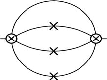
Three of the four propagators of the diagram are differentiated in the mass, i.e. the analytical expression for the propagator in momentum space is $(p^{2}+m^{2})^{-2}$. The reference result of [18] reads

$$B_{N}(0,0,2,2,2,1)=-\frac{7}{4}\zeta(3).$$ (35)

The representation in configuration space for such a diagram (after rotation to Euclidean space-time) has the form

$${\rm wm}4=-4\int_{0}^{\infty}K_{0}(x)^{3}K_{1}(x)x^{2}dx$$ (36)

where the explicit expression for the derivative of the propagator in Eq. (8) with respect to the mass has been used. The diagram is finite (that was the reason for differentiation of the propagators). Therefore the expression for space-time dimension $D=4$ is used. Numerical integration of Eq. (36) gives

$${\rm wm}4=-2.1036\ldots=-\frac{7}{4}\zeta(3)\times[1.0000\ldots\ ]$$ (37)

which coincides with Eq. (35).

We conclude that the configuration space method is simple and rather efficient for numerical computation of diagrams with water melon topology. When the structure of the transcendentality of the result is known for a particular diagram from some other considerations (as in the latest example where only $\zeta(3)$ is present) our numerical technique can be used in some cases to restore the rational coefficients of these transcendentalities which can be thought of as elements of the basis for a class of diagrams.

2.4 Examples in odd-dimensional space-time

It is interesting to note that the computation of Eq. (12) can be performed in closed form for any number of internal lines in space-times of odd dimensions. As the simplest example we take three-dimensional space-time $D\rightarrow D_{0}=3$.

For $\lambda_{0}=(D_{0}-2)/2=1/2$ with $D_{0}=3$ the propagator in Eq. (4) reads

$$D(x,m)\rightarrow D_{3}(x,m)=\frac{\sqrt{mx}K_{1/2}(mx)}{(2\pi)^{3/2}x}=\frac{e^{-mx}}{4\pi x}$$ (38)

while the weight function after the angular integration given by Eq. (13) at $\lambda=\lambda_{0}=1/2$ becomes

$$\left(\frac{px}{2}\right)^{-1/2}J_{1/2}(px)=\frac{2}{\sqrt{\pi}}\frac{\sin(px)}{px}.$$ (39)

The explicit result for the $n$-line water melon diagram is then given by the integral

$$\Pi(p) = 4\pi\int_{0}^{\infty}\frac{\sin(px)}{px}\frac{e^{-Mx}}{(4\pi x)^{n-2}}(\mu x)^{2\epsilon}dx$$ (40)

$$= {\Gamma(2-n+2\epsilon)\over 2ip(4\pi)^{n-1}}\left[(M-ip)^{n-2-2\epsilon}-(M+ip)^{n-2-2\epsilon}\right]\mu^{2\epsilon}$$

where $\epsilon$ is used for regularization and $M=\sum m_{i}$.

Here we see the advantage of using the unorthodox dimensional regularization for computing the finite part of water melon diagrams. The essential simplification of the functional form of the integrand within unorthodox dimensional regularization in odd-dimensional space-time allows one to compute any water melon diagram analytically.

We consider some particular cases of Eq. (40) for different values of $n$. For $n=1$ we simply recover the propagator function with the discontinuity

$$\rho(s)=\frac{\mbox{Disc\,}\Pi(p)}{2\pi i}=\frac{1}{2\pi i}\left(\Pi(p)\Big{|}_{p^{2}=s\exp(-i\pi)}-\Pi(p)\Big{|}_{p^{2}=s\exp(i\pi)}\right)=\delta(s-m^{2})$$ (41)

where $s$ is the squared energy, $s=-p^{2}$. It is usual to call this expression the spectral density associated with the diagram. For $n=2$ the answer for the polarization function $\Pi(p)$ is still finite (no regularization is required) and is given by

$$\Pi(p)=\frac{1}{8\pi ip}\ln\left(\frac{M+ip}{M-ip}\right).$$ (42)

The spectral density, i.e. the discontinuity of Eq. (42) across the cut in the energy square complex $p^{2}$ plane is given by

$$\rho(s)={1\over 8\pi\sqrt{s}}\theta(s-(m_{1}+m_{2})^{2}),\qquad s=-p^{2},\quad s>0$$ (43)

which is nothing but three-dimensional two-particle phase space. This can be immediately checked by direct computation. The cases with $n>2$ have more structure and therefore are more interesting. For the proper sunset diagram with $n=3$, Eq. (40) leads to

$$\Pi(p)=\frac{1}{32\pi^{2}}\left(\frac{1}{\epsilon}-\frac{M}{ip}\ln\left(\frac{M+ip}{M-ip}\right)-\ln\left(\frac{M^{2}+p^{2}}{\mu^{2}}\right)\right).$$ (44)

The arbitrary scale $\mu^{2}$ appears due to our way of regularization. However, the discontinuity of the polarization function in Eq. (44) is independent of $\mu^{2}$ as it must be. The discontinuity is finite and, therefore, independent of the regularization used. Accordingly, Eq. (44) has the correct spectral density,

$$\rho(s)=\frac{\sqrt{s}-M}{32\pi^{2}\sqrt{s}}\,\theta(s-M^{2}).$$ (45)

The general formula for the spectral density for any $n>1$ in $D=3$ can be extracted from Eq. (40). It reads

$$\rho(s)=\frac{(\sqrt{s}-M)^{n-2}}{2(4\pi)^{n-1}(n-2)!\sqrt{s}}\,\theta(s-M^{2}).$$ (46)

We now want to show how the direct subtraction and our unorthodox dimensional regularization are related. Taking Eq. (40) for $n=3$ with a subtraction at the origin, one obtains

$$\Pi(p)=\int_{0}^{\infty}\left(\frac{\sin(px)}{px}-1\right)\frac{e^{-Mx}}{(4\pi)^{2}x}(\mu^{2}x^{2})^{\epsilon}dx$$ (47)

which is UV-finite even for $\epsilon=0$ because there is no singularity at the origin. For practical computations it is convenient to keep the factor $(\mu^{2}x^{2})^{\epsilon}$ in the integrand since this factor gives a meaning to each of the two terms in the round brackets in Eq. (47) separately. Then the direct computation gives

$$\Pi(p) = \int_{0}^{\infty}\left(\frac{\sin(px)}{px}-1\right)\frac{e^{-Mx}}{(4\pi)^{2}x}(\mu^{2}x^{2})^{\epsilon}dx$$ (48)

$$= \frac{\Gamma(-1+2\epsilon)}{2ip(4\pi)^{2}}\left[(M-ip)^{1-2\epsilon}-(M+ip)^{1-2\epsilon}\right]\mu^{2\epsilon}-\frac{\Gamma(2\epsilon)}{(4\pi)^{2}}\left(\frac{\mu}{M}\right)^{2\epsilon}\qquad$$

$$= -\frac{1}{32\pi^{2}}\left\{\frac{M}{ip}\ln\left(\frac{M+ip}{M-ip}\right)+\ln\left(\frac{M^{2}+p^{2}}{M^{2}}\right)\right\}.$$

The poles cancel in this expression and the arbitrary scale $\mu$ changes to $M$. This corresponds to a transition from MS-type of renormalization schemes to a momentum subtraction scheme (with subtraction at the origin in this particular case). Since the spectral density $\rho(s)$ is finite, it can be computed using any regularization scheme as can be seen from Eqs. (44) and (48).

We mention that in the three-dimensional case the spectral density $\rho(s)$ can also be found for general values of $n$ by the traditional methods since the three-dimensional case is sufficiently simple. The use of the convolution equation needed for the evaluation keeps one in the same class of functions, i.e. polynomials in the variable $\sqrt{s}$ divided by $\sqrt{s}$ [20]. The general form of the convolution equation in $D$-dimensional space-time reads

$$\Phi_{n}(s)=\int\Phi_{k}(s_{1})\Phi_{p}(s_{2})\Phi_{2}(s,s_{1},s_{2})ds_{1}ds_{2},\qquad k+p=n.$$ (49)

For the particular case of three-dimensional space-time the kernel $\Phi_{2}(p^{2},m_{1}^{2},m_{2}^{2})$ is given by

$$(2\pi)^{2}\Phi_{2}(p^{2},m_{1}^{2},m_{2}^{2})=\int\delta(k^{2}-m_{1}^{2})\delta((p-k)^{2}-m_{2}^{2})d^{3}k$$ (50)

or, explicitly,

$$\Phi_{2}(s,s_{1},s_{2})=\frac{1}{8\pi\sqrt{s}}\theta(s-(\sqrt{s_{1}}+\sqrt{s_{2}})^{2}).$$ (51)

Eq. (51) can be seen to be the two-particle phase space in three dimensions (cf. Eq. (43)). This is a rather simple example. However, our technique retains its efficiency for large $n$. It is also applicable for odd $D$ other than $3$, say $D=5$. Namely, the propagator in five-dimensional space-time reads ($\lambda_{0}=3/2$)

$$D(x,m)\rightarrow D_{5}(x,m)=\frac{(mx)^{3/2}K_{3/2}(mx)}{(2\pi)^{5/2}x^{3}}=\frac{e^{-mx}}{8\pi^{2}x^{3}}(1+mx)$$ (52)

which assures that the integration in Eq. (12) can be performed in terms of elementary functions (powers and logarithms) again.

We list some potential applications of the general results obtained in this subsection for odd-dimensional space-time. In three space-time dimensions our results can be used to compute phase space integrals for particles in jets where the momentum along the direction of the jet is fixed [21]. Another application can be found in three-dimensional QCD which emerges as the high temperature limit of the ordinary theory of strong interactions for the quark-gluon plasma (see e.g. [9, 22, 23, 24]). Three-dimensional models are also used to study the question of dynamical mass generation and the infrared structure of the models of quantum field theory [25, 26, 27]. A further theoretical application consists in the investigation of properties of baryons in the limit of infinite number of colors $N_{c}\rightarrow\infty$ where one has to take into account the spin structure of internal lines. Note that particular models of different space-time dimensions are very useful because their properties may be simpler and may thus allow one to study general features of the underlying field theory. For example, in six-dimensional space-time the simplest model of quantum field theory $\phi^{3}$ is asymptotically free and can be used for simulations of some features of QCD. Though five-dimensional models are less popular than others, still there are useful applications for Yang-Mills theory in five-dimensional space-time where the UV structure of the models can be analyzed [28].

We conclude this subsection by noting that the $x$-space techniques allow one to compute water melon diagrams in closed form in terms of elementary functions as long as one is dealing with odd-dimensional space-times. The resulting expressions are rather simple and can be directly used for applications. Having the complete formulas at hand, there is no need to expand in the parameters of the diagram such as masses or external momentum. In even number of space-time dimensions there are no closed form solutions in the general case. In this case it is useful to study some limiting configurations. In the next subsection we briefly formulate several limits for water melon diagrams in the Euclidean domain that can be computed analytically with the help of standard integrals given in textbooks [29].

2.5 Limiting configurations and expansions
in the Euclidean domain

What are the advantages of our method, especially for even dimensions? We shall find that, compared to existing approaches, our method results in great simplifications in computing the polarization function in the Euclidean domain. While the basic representation in Eq. (12) can always be used for numerical evaluations, some analytical results can be obtained for particular choices of the parameters in the diagram (i.e. masses and external momenta). Different regimes can be considered and some cases can be explicitly done in closed form.

The simplest case is the limit of one large mass and all other masses being small. For the polarization function in the Euclidean domain this limit is easy to compute because of the simplicity of the $x$-space representation and the high speed of convergence of the ensuing numerical procedures. But this special limit can also be done analytically. When expanding the propagators in the limit of small masses one encounters powers of $x$ and $\ln(mx)$. The remaining functions are the weight function (the Bessel function) and the propagator of the heavy particle with the large mass $M_{h}$ which is given by the McDonald function. The general structure of the terms in the series expansion that contribute to $\Pi(p)$ is given by

$$2\pi^{\lambda+1}\int_{0}^{\infty}\left(\frac{px}{2}\right)^{-\lambda}J_{\lambda}(px)K_{\nu}(M_{h}x)x^{2\rho}\ln^{j}(mx)dx,\quad\rho,j\geq 0.$$ (53)

The integrations in (53) can be done in closed form by using the basic integral representation

$$\int_{0}^{\infty}x^{\mu}J_{\lambda}(px)K_{\nu}(M_{h}x)dx$$ (54)

$$= \frac{p^{\lambda}\Gamma((\lambda+\mu+\nu+1)/2)\Gamma((\lambda+\mu-\nu+1)/2)}{2^{1-\mu}M_{h}^{\lambda+\mu+1}\Gamma(\lambda+1)}$$

$$\qquad{}_{2}F_{1}\left((\lambda+\mu+\nu+1)/2,(\lambda+\mu-\nu+1)/2;\lambda+1;-p^{2}/M_{h}^{2}\right)$$

where ${}_{2}F_{1}(a,b;c;z)$ is the usual hypergeometric function [29]. The corresponding integrals with integer powers of logarithms ($j>0$ in Eq. (53)) can be obtained by differentiation with respect to $\mu$. Note that the maximal power of the logarithm is determined by the number of light propagators and does not increase with the order of the expansion: any light propagator contains only one power of the logarithm as follows from the expansion of the McDonald function $K_{\nu}(\xi)$ at small $\xi$ [29].

The basic formula Eq. (12) is also well suited for finding $p^{2}$-derivatives of the polarization function $\Pi(p)$. The values of the polarization function and its derivatives at $p^{2}=0$ can be easily obtained. The convenience of a $p^{2}$ expansion is demonstrated by making use of the basic formula for differentiating the Bessel function,

$$\frac{d^{k}}{d(p^{2})^{k}}\left(\frac{px}{2}\right)^{-\lambda}J_{\lambda}(px)=(-x^{2})^{k}\left(\frac{px}{2}\right)^{-\lambda-k}J_{\lambda+k}(px).$$ (55)

Note that differentiation results in an expression which has the same functional structure as the original function. This is convenient for numerical computations. Note that sufficiently high order derivatives become UV-finite (operationally it is clear since the subtraction polynomial vanishes after sufficiently high derivatives are taken). This can also be seen explicitly from Eq. (55) where high powers of $x^{2}$ suppress the singularity of the product of propagators at small $x$.

Mass corrections to the large $p^{2}$ behaviour in the Euclidean domain (an expansion in $m_{i}^{2}/p^{2}$) are obtained by expanding the massive propagators in terms of masses $m_{i}$ under the integration sign. The final integration is performed by using the formula

$$\int_{0}^{\infty}x^{\mu}J_{\lambda}(px)dx=2^{\mu}p^{-\mu-1}\frac{\Gamma\left({\lambda+\mu+1\over 2}\right)}{\Gamma\left({\lambda-\mu+1\over 2}\right)}.$$ (56)

Note that all these manipulations are straightforward and can be easily implemented in a system of symbolic computations. Some care is necessary, though, when poles of the $\Gamma$-function are encountered which reflect the appearance of artificial infrared singularities. The corresponding framework for dealing with such problems is well known (see e.g. [30, 31]).

3 Analytic continuation in momentum space

Now we consider an explicit analytic continuation in the complex $p^{2}$ plane and locate the discontinuity of the polarization function which is nothing but the spectral density $\rho(s)$. Note that the spectral density represents $n$-particle phase space for the water melon configuration.

Again we use the basic formula given by Eq. (12) for analytic continuation. The spectral density reads

$$\rho(s) = \frac{i}{2\pi}\int_{0}^{\infty}\left(\frac{2\pi\xi}{s}\right)^{\lambda+1}J_{\lambda}(\xi)\Bigg{[}e^{-i\pi(\lambda+1)}\prod_{i=1}^{n}\frac{1}{4}\left(\frac{m_{i}\sqrt{s}}{2\pi\xi}\right)^{\lambda}e^{i\pi(\lambda+1/2)}H^{(1)}_{\lambda}\left(\frac{m_{i}\xi}{\sqrt{s}}\right)$$ (57)

$$\qquad\qquad-e^{i\pi(\lambda+1)}\prod_{i=1}^{n}\frac{1}{4}\left(\frac{m_{i}\sqrt{s}}{2\pi\xi}\right)^{\lambda}e^{-i\pi(\lambda+1/2)}H^{(2)}_{\lambda}\left(\frac{m_{i}\xi}{\sqrt{s}}\right)\Bigg{]}d\xi.$$

The analytic continuation is performed using the result

$$K_{\lambda}(z)=\frac{\pi i}{2}e^{\frac{\pi}{2}\lambda i}H^{(1)}_{\lambda}(iz)$$ (58)

where $H^{(1,2)}_{\lambda}(z)$ are the Hankel functions, $H^{(1)}_{\lambda}(z)=(H^{(2)}_{\lambda}(z))^{*}$ for real $z,\lambda$ [29]. We have thus obtained an explicit representation for the spectral density in terms of a one-dimensional integral representation. Using Eq. (57) one can easily discuss special mass configurations. It is understood that the UV subtraction has been performed in Eq. (57), i.e. the kernel $(\xi/2)^{-\lambda}J_{\lambda}(\xi)$ is substituted with the subtracted one $[.]_{N}$ from Eq. (14).

A remark about the numerical evaluation of the integrals in Eq. (57) is in order. As our main purpose is to create a practical tool for evaluation of the water melon class of diagrams, we do not insist on an analytical evaluation of the integrals in Eq. (57). This issue will be discussed in more detail in Sec. 4. The one-dimensional integral representation in Eq. (57) is simple enough for further processing. The evaluation of the integral in Eq. (57) is, however, not always straightforward. The integrand contains highly oscillating functions that require some care in the numerical treatment. This is to be expected since the discontinuity, or the spectral density, is a distribution rather than a smooth function. However, because the analytic structure and the asymptotic behaviour of the integrand in Eq. (57) is completely known, the numerical computation of $\rho(s)$ can be made reliable and fast in domains where $\rho(s)$ is smooth enough, in particular far from threshold. One recipe is to extract the oscillating asymptotics first and then to perform the integration analytically, or to integrate the oscillating asymptotics numerically using integration routines that have special options for the treatment of oscillatory integrands. Both ways were checked in simple examples with reliable results. The remaining non-oscillating part is a slowly changing function which can be integrated numerically without difficulties. With this extra care the integration can be easily made safe, reliable and fast even for an average personal computer. We mention that we have checked our general numerical procedures in three-dimensional space-time ($D_{0}=3$) where exact results are available (see Sec. 2).

As an example of the efficiency of our technique we take Eq. (57) to recompute the spectral density of the $n=3$ water melon diagram for three-dimensional space-time. The Hankel function for indices $j+1/2$ (or for $D_{0}=2j+1$) is a finite combination of powers and an exponential which makes possible the explicit computation of the integral in Eq. (57). In fact, for this case one has

$$\rho(s)=-\frac{1}{\pi}\int_{0}^{\infty}\left(\frac{\sin\xi}{\xi}-1\right)\sin\left(\frac{M\xi}{\sqrt{s}}\right)\frac{d\xi}{(4\pi)^{2}\xi}=\frac{\sqrt{s}-M}{32\pi^{2}\sqrt{s}}\,\theta(s-M^{2}).$$ (59)

This form coincides with the explicit formulas given by Eqs. (42) and (43). The generalization to higher $n$ includes only algebraic manipulations. The necessary integrations corresponding to the one in Eq. (59) are performed by moving the contour into the complex $\xi$-plane and regularizing the singularity at the origin by an infinitely small shift $\pm i0$. Then closing the contour in the upper or lower semi-plane according to the sign of regularization one finds the integral by computing the residue at the origin. Note that an explicit subtraction is kept in Eq. (59).

The results for the spectral density for $n=3$ and $4$ can be obtained directly by making use of traditional techniques as well. One obtains a one-dimensional integral representation for $n=3$ and a two-dimensional integral representation for $n=4$ [20]. For larger $n$, however, the corresponding technique of convolution includes many-fold integrals and the corresponding recursion relation (49) is not convenient for applications. This has to be contrasted with the one-dimensional integral representation in Eq. (57) derived here which allows one to compute the spectral density for the class of water melon diagrams with large number of internal lines in any number of space-time dimensions.

4 Integral transformation in configuration space

The analytic structure of the correlator $\Pi(x)$ (or the spectral density of the corresponding polarization operator) can be determined directly in configuration space without having to compute its Fourier transform first. The dispersion representation (or the spectral decomposition) of the polarization function in configuration space has the form

$$\Pi(x)=\int_{0}^{\infty}\rho(m^{2})D(x,m)dm^{2}$$ (60)

where for this section we switch to a notation where $\sqrt{s}=m$. This representation was used for sum rules applications in [32, 33] where the spectral density for the two-loop sunset diagram was found in two-dimensional space-time [34]. With the explicit form of the propagator in configuration space given by Eq. (4), the representation in Eq. (60) turns into a particular example of the Hankel transform, namely the $K$-transform [35, 36]. Up to inessential factors of $x$ and $m$, Eq. (60) reduces to the generic form of the $K$-transform for a conjugate pair of functions $f$ and $g$,

$$g(y)=\int_{0}^{\infty}f(x)K_{\nu}(xy)\sqrt{xy}\,dx.$$ (61)

The inverse of this transform is known to be given by

$$f(x)=\frac{1}{\pi i}\int_{c-i\infty}^{c+i\infty}g(y)I_{\nu}(xy)\sqrt{xy}\,dy$$ (62)

where $I_{\nu}(x)$ is a modified Bessel function of the first kind and the integration runs along a vertical contour in the complex plane to the right of the right-most singularity of the function $g(y)$ [36]. In order to obtain a representation for the spectral density $\rho(m^{2})$ of a water melon diagram in general $D$-dimensional space-time one needs to apply the inverse $K$-transform to the particular case given by Eq. (60). One has

$$m^{\lambda}\rho(m^{2})=\frac{(2\pi)^{\lambda}}{i}\int_{c-i\infty}^{c+i\infty}\Pi(x)x^{\lambda+1}I_{\lambda}(mx)dx.$$ (63)

The inverse transform given by Eq. (63) solves the problem of determining the spectral density of water melon diagrams by reducing it to the computation of a one-dimensional integral for the general class of water melon diagrams with any number of internal lines and different masses. Compared to the general solution given by Eq. (57) the above form is simpler. Below we discuss some technicalities concerning the efficient evaluation of the contour integral in the representation given by Eq. (63). The analytic structure of the correlator in Eq. (3) is now explicit using the representation given by Eq. (63) and exhibits the distribution nature of the spectral density $\rho(m^{2})$ as shown below.

Note that the expression given by Eq. (3) can have non-integrable singularities at small $x$ for a sufficiently large number of propagators when $D>2$ [16]. Therefore the computation of its Fourier transform requires regularization or subtractions [37]. The spectral density itself is finite (the structure of the water melon diagrams is very simple and there are no subdivergences when one employs a properly defined $R$-operation [16]) and thus requires no regularization. In the more traditional approach of direct analytic continuation in momentum space the explicit representation for the spectral density is given by Eq. (57) where one has taken the discontinuity of the Fourier transform across the physical cut for $p^{2}=-m^{2}\pm i0$. This is an alternative representation of the spectral density, and in some instances the latter representation can be more convenient for numerical treatment.

In the following we present some explicit examples of applying the technique of computing the spectral density of water melon diagrams on the basis of integral transforms in configuration space.

4.1 One-loop case

First a remark about the mass degenerate one-loop case is in order. All necessary integrals (both for the direct and the inverse $K$-transform) involve no more than the product of three Bessel functions which can be found in a standard collection of formulas for special functions (see e.g. [29]). The spectral density in $D$-dimensional space-time (for two internal lines with equal masses $m_{0}$) can be computed to be

$$\rho(m^{2})=\frac{(m^{2}-4m_{0}^{2})^{\lambda-1/2}}{2^{4\lambda+1}\pi^{\lambda+1/2}\Gamma(\lambda+1/2)m},\qquad m>2m_{0}.$$ (64)

This formula is useful since it can be used to test the limiting cases of more general results.

The corresponding spectral density for the nondegenerate case with two different masses $m_{1}$ and $m_{2}$ reads

$$(2\pi)^{2\lambda+1}\rho(m^{2})=\frac{\Omega_{2\lambda+1}}{4m}\left(\frac{(m^{2}-m_{1}^{2}-m_{2}^{2})^{2}-4m_{1}^{2}m_{2}^{2}}{4m^{2}}\right)^{\lambda-1/2},\qquad m>m_{1}+m_{2},$$ (65)

where

$$\Omega_{d}=\frac{2\pi^{d/2}}{\Gamma(d/2)}$$ (66)

is a volume of a unit sphere in $d$-dimensional space-time. Note the identity

$$(m^{2}-m_{1}^{2}-m_{2}^{2})^{2}-4m_{1}^{2}m_{2}^{2}=\left[m^{2}-(m_{1}+m_{2})^{2}\right]\left[m^{2}-(m_{1}-m_{2})^{2}\right]$$ (67)

which immediately allows one to locate the two-particle threshold.

4.2 Odd-dimensional case

For odd-dimensional space-time the representation in Eq. (60) reduces to the ordinary Laplace transformation. To obtain the spectral density (the function $f(x)$ in this particular example) one can use Eq. (62). For energies below threshold it is possible to close the contour of integration to the right. With the appropriate choice of the constant $c$ as specified above, the closed contour integration gives zero due to the absence of singularities in the relevant domain of the right semi-plane. By closing the contour of integration to the left and keeping only that part of the function $I_{\nu}(z)$ which is exponentially falling for ${\rm Re}(z)<0$ one can obtain another convenient integral representation for the spectral density when the energy is above threshold. The only singularities within the closed contour are then poles at the origin (in odd-dimensional space-time) and the evaluation of the integral can be done by determining the corresponding residues. These are purely algebraic manipulations, the simplicity of which also explain the simplicity of the computations in odd-dimensional space-time. For a small number of internal lines $n$ the spectral density can also be found by using the convolution formulas for the spectral densities of a smaller number of particles (see e.g. [20]). For large $n$ the computations described in [20] become quite cumbersome and the technique suggested in the present paper is much more convenient.

As an example for the odd-dimensional case we present calculations in three dimensions. The dispersion representation for three-dimensional space-time has the following form

$$\Pi(x)=\int_{0}^{\infty}\rho(m^{2})D_{3}(x,m)dm^{2}=\int_{0}^{\infty}\rho(m^{2}){e^{-mx}\over 4\pi x}dm^{2}$$ (68)

with the three-dimensional scalar propagator

$$D_{3}(x,m)=\frac{\sqrt{mx}K_{1/2}(mx)}{(2\pi)^{3/2}x}=\frac{e^{-mx}}{4\pi x}.$$ (69)

One can invert Eq. (68) and obtains

$$2m\rho(m^{2})=\frac{1}{2\pi i}\int_{c-i\infty}^{c+i\infty}4\pi x\Pi(x)e^{mx}dx$$ (70)

which is a special case of Eqs. (62) and (63) with

$$I_{\frac{1}{2}}(z)=\sqrt{\frac{2}{\pi z}}\sinh(z)$$ (71)

where one only needs to retain the $e^{z}$ piece in the hyperbolic sine function. The solution given by Eq. (70) has the appropriate support as a distribution or, equivalently, as an inverse Laplace transform. It vanishes for $m<M=\sum_{i=1}^{n}m_{i}$ since the contour of integration can be closed to the right where there are no singularities of the integrand. Recall that for large $x$ with ${\rm Re}(x)>0$ the asymptotic behaviour of the polarization function $\Pi(x)$ is governed by the sum of the masses of the propagators and reads

$$\Pi(x)\sim\exp{(-xM)}.$$ (72)

For $m>M$ one can close the contour to the left in the complex $x$-plane and then the only singularities of $\Pi(x)$ are the poles at the origin of $\Pi(x)$ since $\Pi(x)$ is a product of the propagators of the form of Eqs. (3) and (69). The integration in Eq. (70) then reduces to finding the residues of the poles at the origin. Indeed,

$$\Pi(x)=\prod_{i=1}^{n}D_{3}(x,m_{i})={e^{-Mx}\over(4\pi x)^{n}},$$ (73)

and Eq. (70) gives an explicit representation of the spectral density through the polarization function in $x$-space,

$$2m\rho(m^{2})=\frac{1}{2\pi i}\int_{c-i\infty}^{c+i\infty}4\pi x\Pi(x)e^{mx}dx=\frac{1}{2\pi i(4\pi)^{n-1}}\int_{c-i\infty}^{c+i\infty}\frac{e^{(m-M)x}}{x^{n-1}}dx.$$ (74)

In closing the contour of integration to the left one computes the residue at the origin and obtains ($n>1$)

$$2m\rho(m^{2})=\frac{(m-M)^{n-2}}{(4\pi)^{n-1}(n-2)!}\theta(m-M).$$ (75)

Eq. (75) coincides with the expression (46). This also explains the simplicity of the structure of the spectral density in odd numbers of dimensions of space-time when traditional means are used [37]. In five-dimensional space-time Eq. (70) is applicable almost without any change because the propagator now reads

$$D_{5}(x,m)=\frac{(mx)^{3/2}K_{3/2}(mx)}{(2\pi)^{5/2}x^{3}}=\frac{e^{-mx}}{8\pi^{2}x^{3}}(1+mx).$$ (76)

Compared to the three-dimensional case the only additional complication is that the order of the pole at the origin is changed and that one now has a linear combination of terms instead of the simple monomial in three dimensions.

4.3 Even-dimensional case

For even-dimensional space-time the analytic structure of $\Pi(x)$ in Eq. (3) is more complicated. There is a cut along the negative axis in the complex $x$-plane which prevents a straightforward evaluation by simply closing the contour of integration to the left (with ${\rm Re}(x)<0$). The discontinuity along the cut is, however, well known and includes only Bessel functions that appear in the product of propagators for the polarization function. Therefore the representation (63) is essentially equivalent to the direct analytic continuation of the Fourier transform [37] but may be more convenient for numerical treatment because there is no oscillating integrand in (63).

In even number of dimensions one is thus dealing with a genuine $K$-transform. We discuss in some detail the important case of four-dimensional space-time. For $D=4$ ($\lambda=1$), Eqs. (4) and (60) give

$$\Pi(x)=\int\rho(m^{2})D_{4}(x,m)dm^{2}=\int\rho(m^{2})\frac{mxK_{1}(mx)}{4\pi^{2}x^{2}}dm^{2},$$ (77)

and Eq. (63) is written as

$$2m\rho(m^{2})=\frac{1}{\pi i}\int_{c-i\infty}^{c+i\infty}4\pi^{2}x^{2}\Pi(x)I_{1}(mx)dx.$$ (78)

All remarks about the behaviour at large $x$ apply here as well. However, the structure of singularities is more complicated than in the odd-dimensional case. In addition to the poles at the origin there is a cut along the negative axis that renders the computation of the spectral density more difficult. The cut arises from the presence of the functions $K_{1}(m_{i}x)$ in the polarization function $\Pi(x)$. Also the asymptotic behaviour of the function $I_{1}(z)$ is more complicated than that of $I_{1/2}(z)$. In particular the extraction of the exponentially falling component on the negative real axis is not straightforward. Incidentally, the fall-off behaviour of the function $I_{1}(z)$ on the negative real axis can be taken as an example of Stokes’ phenomenon of asymptotic expansions (see e.g. [12]). While the analytic structure of the representation is quite transparent and the integration can be performed along a contour in the complex plane, there are some subtleties when one wants to obtain a convenient form for numerical treatment analogous to odd-dimensional case  [37].

After closing the contour to the left (for $m>M$) using the appropriate part of the function $I_{1}(z)$ we obtain

$$i\pi\int_{c-i\infty}^{c+i\infty}x^{2}\Pi(x)I_{1}(mx)dx$$

$$= -\int_{\epsilon}^{\infty}r^{2}\left(\Pi(e^{i\pi}r)+\Pi(e^{-i\pi}r)\right)K_{1}(mr)dr+2\int_{\epsilon}^{\infty}r^{2}\Pi(r)K_{1}(mr)dr$$

$$+\int_{C_{-}}z^{2}\Pi(z)(i\pi I_{1}(mz)+K_{1}(mz))dz+\int_{C_{+}}z^{2}\Pi(z)(i\pi I_{1}(mz)-K_{1}(mz))dz$$

for the quantity entering Eq. (78). The contours $C_{+}$ and $C_{-}$ are semi-circles of radius $\epsilon$ around the origin in the upper and lower complex semi-plane, respectively (see Fig. 3).

Figure 3: Integration contours used in the evaluation of Eq. (4.3). $R_{1}$, $R_{2}$, $R_{3}$ and $R_{4}$ are segments of a circle arround the origin where the radius of the circle is taken to infinity

For practical evaluations of $\Pi(e^{\pm i\pi}r)$ the following rule for the analytic continuation of the McDonald functions is used,

$$K_{1}(e^{\pm i\pi}\xi)=-K_{1}(\xi)\mp i\pi I_{1}(\xi),\qquad\xi=mr>0.$$ (80)

Some comments are in order. The polarization function $\Pi(z)$ at $z=e^{\pm i\pi}r$ is proportional to the product of propagators of the form

$$D_{4}(e^{\pm i\pi}r,m_{i})\sim\frac{m_{i}}{r}\left[K_{1}(m_{i}r)\pm i\pi I_{1}(m_{i}r)\right].$$ (81)

It is clear from this equation that the leading singular contribution proportional to the product of $K_{1}(m_{i}r)$ cancels in the sum in Eq. (4.3). Also the next-to-leading singular term disappears because of different signs in the product. Recall that the small $\xi$ behaviour of the functions $K_{1}(\xi)$ and $I_{1}(\xi)$ is given by

$$K_{1}(\xi)=\frac{1}{\xi}+O(\xi\ln\xi),\quad I_{1}(\xi)=\frac{\xi}{2}+O(\xi^{3}).$$ (82)

Let us add a few remarks on the final representation Eq. (4.3) which is in a suitable form for numerical integration. We have introduced an auxiliary regularization in terms of a circle of finite radius $\epsilon$ which runs around the origin with its pole-type singularities. The spectral density is independent of $\epsilon$, and the parameter $\epsilon$ completely cancels in the full expression for the spectral density as given by Eq. (4.3). This must be so since the spectral density is finite for the class of water melon diagrams. Eq. (4.3) contains no oscillatory integrands (cf. Eq. (57)), and the integration can safely be done numerically. Thus Eq. (4.3) is a useful alternative representation for the spectral density. In practice the integration over the semi-circles is done by expanding the integrand in $z$ for small $z$ and keeping only terms singular in $\epsilon$. The expansion requires only a finite number of terms and is a purely algebraic operation. Then the singularity in $\epsilon$ exactly cancels against those of the remaining integrals. This cancellation can also be done analytically leaving well defined and smooth integrands for further numerical treatment.

Even if the full computation of the spectral function in the even-dimensional case described here is straightforward it is nevertheless cumbersome. In order to exhibit the essential points in this calculation we illustrate it with a simple and instructive example. Consider the calculation of the following integral

$$\int_{c-i\infty}^{c+i\infty}\frac{\ln z}{z^{2}}e^{z}dz$$ (83)

which is rather close in structure to the real case. Due to the singularity at the origin one has to treat the vicinity of the origin carefully. We proceed by closing the contour to the left

$$\int_{c-i\infty}^{c+i\infty}\frac{\ln z}{z^{2}}e^{z}dz = \int_{C_{\epsilon}}\frac{\ln z}{z^{2}}e^{z}dz-\int_{\epsilon}^{\infty}\frac{2i\pi}{x^{2}}e^{-x}dx$$ (84)

$$= -2\pi i\int_{\epsilon}^{\infty}{e^{-x}dx\over x^{2}}+i\int_{-\pi}^{\pi}{\ln\epsilon+i\phi\over\epsilon}(1+\epsilon e^{i\phi})e^{-i\phi}d\phi$$

$$= -2\pi i\int_{\epsilon}^{\infty}{e^{-x}dx\over x^{2}}+i\int_{-\pi}^{\pi}\left({\ln\epsilon\over\epsilon}e^{-i\phi}+{i\phi\over\epsilon}e^{-i\phi}+\ln\epsilon+i\phi\right)d\phi$$

$$= -2\pi i\int_{\epsilon}^{\infty}{e^{-x}dx\over x^{2}}+{\ln\epsilon\over\epsilon}0+{2\pi i\over\epsilon}+2\pi i\ln\epsilon+0$$

$$= -2\pi i\left(\int_{\epsilon}^{\infty}{e^{-x}dx\over x^{2}}-{\frac{1}{\epsilon}}-\ln\epsilon\right)\,.$$

The combination in the brackets of the last equation remains finite as $\epsilon\rightarrow 0$. Let us now consider this limit in more detail. First we split the integration into two parts from $\epsilon$ to $1$ and from $1$ to infinity,

$$\int_{\epsilon}^{\infty}{e^{-x}dx\over x^{2}}=\int_{1}^{\infty}{e^{-x}dx\over x^{2}}+\int_{\epsilon}^{1}{e^{-x}dx\over x^{2}}.$$ (85)

Then the first integral is just a number which can be found numerically with high precision. In the second integral we can expand the exponent in the integrand and find

$$\int_{\epsilon}^{1}{e^{-x}dx\over x^{2}}=\int_{\epsilon}^{1}{dx\over x^{2}}(1-x+\frac{x^{2}}{2}-\ldots)=\frac{1}{\epsilon}-1+\ln{\epsilon}+\frac{1}{2}(1-\epsilon)+\ldots.$$ (86)

The singularity has the correct form and the finite series converges well. If one takes a value $0.1$ instead of $1$ for the splitting point in Eq. (85) the convergence of the finite series will be very fast. This procedure would be used for practical integration in a realistic case.

Now we give an exact answer for our simple example. After two integrations by parts we have

$$\int_{\epsilon}^{\infty}{e^{-x}dx\over x^{2}}=e^{-\epsilon}\left(\frac{1}{\epsilon}+\ln{\epsilon}\right)-\int_{\epsilon}^{\infty}e^{-x}\ln xdx.$$ (87)

The last integral is finite at $\epsilon=0$ and for our purpose it suffices to compute it in this limit. The result is

$$\int_{0}^{\infty}e^{-x}\ln x\,dx=-\gamma_{E}$$ (88)

where $\gamma_{E}$ is again the Euler’s constant. All these manipulations can be easily done with a symbolic program. For the original integral one finds

$$-2\pi i\left(\int_{\epsilon}^{\infty}{e^{-x}dx\over x^{2}}-{\frac{1}{\epsilon}}-\ln\epsilon\right) = -2\pi i\left(e^{-\epsilon}\left(\frac{1}{\epsilon}+\ln{\epsilon}\right)+\gamma_{E}-{\frac{1}{\epsilon}}-\ln\epsilon\right)$$ (89)

$$= 2\pi i(1-\gamma_{E})\quad\mbox{at}\quad\epsilon=0.$$

Thus finally

$$\int_{c-i\infty}^{c+i\infty}\frac{\ln z}{z^{2}}e^{z}dz=2\pi i(1-\gamma_{E})\,.$$ (90)

This concludes our discussion of how to treat subtractions in this simplified case. The generalization to Bessel functions is straightforward (just expand near the origin and get expressions as in Eq. (84)). Then the form of the subtraction term depends on the number $n$ of propagators in a water melon diagram. Writing down an explicit expression for some $n$ is routine and we leave it to the interested user. All the required expansions can be performed by a symbolic manipulation program.

Again for $n=3$ the results for the spectral density can be obtained directly by traditional means through the convolution equation (49). It leads to a one-dimensional integral representation for $n=3$. In this respect the representation in Eq. (4.3) is of the same level of complexity while the convolution equation is even simpler because it includes only an integration over a finite interval. However, for $n=4$ the convolution equation leads to a two-dimensional integral representation [20]. For larger $n$ the corresponding technique of convolution includes many-fold integrals and the corresponding recursion relation in Eq. (49) is not very convenient for applications. In the configuration space approach all formulas remain the same regardless of the number $n$ of internal lines and thus this approach must be considered to be superior to the more traditional momentum space approach.

For two-dimensional space-time the representation analogous to Eq. (4.3) is simpler because there is no power singularity at the origin but only a logarithmic singularity which allows one to shrink the contour to a point (take the limit $\epsilon\rightarrow 0$). In this case we obtain

$$\rho(m^{2})=\frac{1}{\pi}\int_{0}^{\infty}r(2\Pi(r)-\Pi(e^{i\pi}r)-\Pi(e^{-i\pi}r))K_{0}(mr)dr.$$ (91)

For $D_{0}=2$ we present our results for the cases $n=2$ and $n=3$. For the one-loop case $n=2$ one has

$$\rho(m^{2})=\frac{1}{2\pi}\int_{0}^{\infty}rI_{0}(m_{1}r)I_{0}(m_{2}r)K_{0}(mr)dr$$ (92)

which can be integrated explicitly and results in [19]

$$\rho(m^{2})=\frac{1}{2\pi m^{2}}\sum_{k,l=0}^{\infty}\left(\frac{(k+l)!}{k!l!}\right)^{2}\left(\frac{m_{1}^{2}}{m^{2}}\right)^{k}\left(\frac{m_{2}^{2}}{m^{2}}\right)^{l}.$$ (93)

This series can of course also be directly obtained by expanding Eq. (65).

For the case $n=3$ one obtains

$$\rho(m^{2}) = \frac{1}{(2\pi)^{2}}\int_{0}^{\infty}r(K_{0}(m_{1}r)I_{0}(m_{2}r)I_{0}(m_{3}r)+I_{0}(m_{1}r)K_{0}(m_{2}r)I_{0}(m_{3}r)$$ (94)

$$\qquad\qquad+I_{0}(m_{1}r)I_{0}(m_{2}r)K_{0}(m_{3}r))K_{0}(mr)dr.$$

Again, this result can be obtained by an alternative method, i.e. by making use of the convolution equation given in Eq. (49). The $\delta$-function $\Phi_{1}(m^{2})=\delta(m^{2}-m_{3}^{2})$ is the spectral density of the additional internal line with mass $m_{3}$. $\Phi_{2}(m^{2})$ and $\Phi_{2}(m^{2},m_{1}^{2},m_{2}^{2})$ are the one-loop spectral density given by Eq. (65). In performing the convolution one obtains

$$\rho(m^{2})=\frac{1}{(2\pi)^{2}}\int_{(m_{1}+m_{2})^{2}}^{(m-m_{3})^{2}}\frac{ds_{1}}{\sqrt{((s_{1}-m_{1}^{2}-m_{2}^{2})^{2}-4m_{1}^{2}m_{2}^{2})((m^{2}-s_{1}-m_{3}^{2})^{2}-4s_{1}m_{3}^{2})}}.$$ (95)

The integrand in Eq. (95) is singular at the end points and a numerical evaluation requires some care. Contrary to this, there are no problems when Eq. (94) is used. With modern computer facilities, the integral representation given in Eq. (94) is more suitable for a numerical evaluation than the form given by Eq. (95).

The most direct and efficient way of numerical evaluation of the spectral density is the immediate use of Eq. (63). After choosing the contour to be a straight vertical line in the complex $x$-plane with some positive $c$ and making change of the variable $x=c+iy$ the integration over $y$ is straightforward. For large number of lines $n$ in a water melon diagram the convergence of the integral becomes fast because the integrand falls off as $|y|^{-3(n-1)/2}$ at large $|y|$. One finds several correct decimal figures of the result rather easily using an ordinary personal computer. A good check for the quality of numerical results obtained in this way is their independence of $c$. The results must be the same for any particular choice of $c$.

4.4 Threshold behaviour

Finally we return to the threshold behaviour of the spectral density. Using the results of the above analysis one arrives at expressions of the general form

$$2m\rho(m^{2})\sim\int^{\infty}K_{1}(mr)\prod_{i}Z_{1}(m_{i}r)dr$$ (96)

where $Z_{1}(m_{i}r)$ is either $I_{1}(m_{i}r)$ or $K_{1}(m_{i}r)$. The convergence at large $r>0$ (at the upper limit of the integral) is controlled by the factor $\exp{(-(m-M)r)}$ as in Eq. (74), and the corresponding expansions in the variable $m-M$ in the region $m\sim M$ can be constructed. As shown before, the spectral density for odd-dimensional space-time is known exactly. Its threshold behaviour is easily extracted and one obtains

$$\rho(m^{2})\approx\frac{(m-M)^{n-2}}{2m(4\pi)^{n-1}(n-2)!}$$ (97)

at $m$ close to $M$.

In the realistic case of four-dimensional space-time the threshold behaviour of the spectral density can be inferred from Eq. (63) (and, also, Eq. (96)). Substituting the asymptotic limit of modified Bessel functions at large arguments we infer from the simple dimensional considerations that

$$\rho(m^{2})\sim(m-M)^{(3n-5)/2}$$ (98)

at $m$ close to $M$, where $n$ is the number of internal lines of the water melon diagram. One obtains $\rho(m^{2})\sim\sqrt{m-M}$ for $n=2$ and $\rho(m^{2})\sim(m-M)^{2}$ for $n=3$ at $m$ close to $M$. The threshold behaviour agrees with the one extracted from the explicit formula given by Eq. (64) or with the threshold behaviour derived from the convolution equation in Eq. (49). Other space-time dimensions can be analyzed along the same lines.

For the sake of completeness we briefly comment on the opposite limit for the spectral density when $m^{2}\rightarrow\infty$. In this limit the external energy is much larger than all masses. The limiting behaviour of this kinematic configuration can be found by utilizing the massless approximation for the correlator where analytical expressions are available. Subleading corrections can be obtained using known techniques [4].

5 Conclusion

We have described a novel technique that reduces the computation of any water melon diagram to a simple one-dimensional integral with known functions in the integrand. Additional tensor and form factor structures can be easily included without modification of the basic formulas. Different regimes of behaviour with respect to mass/momentum expansions can be easily analyzed and the results can be found analytically if no more than two dimensionful parameters (one mass and momentum or two masses) are treated exactly and other parameters are considered to be small and are treated in series expansions. Explicit analytical formulas (with even that last integration being performed in closed form) are given for the case of any odd number of space-time dimensions. The analytic continuation to the Minkowskian region, i.e. to the positive $s$-axis has been performed and the discontinuity across the physical cut is explicitly given. This allows one to compute general $n$-particle phase space for any kind of particles both with different masses and Lorentz structures. The threshold behaviour of the spectral density can be easily investigated based on such a representation. In the even-dimensional case the final integration for an arbitrary water melon diagram was not done explicitly since we encountered products of Bessel functions which we were unable to integrate in a closed form. This forces one to use numerical integrations in the even-dimensional case if numerical results are desired for large $n$. However, the analytic structure of the solution for the diagram is fully determined which makes the numerical treatment rather reliable and fast. In this sense the computation of water melon diagrams has been converted to the routine procedure of getting numbers. Except for some special cases the final one-dimensional integral representation was not further reduced to known simpler functions. This is quite familiar from the theory of special functions where many special functions are represented through one-dimensional integrals which cannot be further reduced to known functions. In this sense our formulas completely solve the problem of computing the class of water melon diagrams.

Well, the water melon is finished and the sunset is over long ago. So the next story has to wait until the next sunrise takes place.

Acknowledgments
We thank A. Davydychev for useful comments on the literature related to the subject of the present paper. We futher thank D. Broadhurst for an interesting discussion. A. Grozin has provided us with the program RECURSOR [18] which allowed us to obtain the analytical result in Eq. (35). The work is supported in part by the Volkswagen Foundation under contract No. I/73611. A.A. Pivovarov is supported in part by the Russian Fund for Basic Research under contracts Nos. 96-01-01860 and 97-02-17065.

References

- [1] G. Altarelli, T. Sjöstrand and F. Zwirner (Eds.), Proceedings of the CERN workshop “Physics at LEP2”, 2–3 Feb. 1995, Geneva, Switzerland, CERN, 1996
- [2] N.V.Krasnikov and V.A.Matveev, “Physics at LHC”, Phys. Part. Nucl. 28 (1997) 441
- [3] Particle Data Group, “ Review of Particle Properties”, Eur. Phys. J. C3 (1998) 1
- [4] K.G. Chetyrkin, J.H. Kühn and A. Kwiatkowski, Phys. Rep. 277 (1996) 189
- [5] L. Brücher, J. Franzkowski and D. Kreimer, “X-loops: A program package calculating one-loop Feynman diagrams”, Report No. MZ-TH-97-35, hep-ph/9710484
- [6] F.A. Berends, M. Buza, M. Böhm and R. Scharf, Z. Phys. C63 (1994) 227
- [7] P. Post and K. Schilcher, Phys. Rev. Lett. 79 (1997) 4088
- [8] P. Post and J.B. Tausk, Mod. Phys. Lett. A11 (1996) 2115
- [9] A.K. Rajantie, Nucl. Phys. B480 (1996) 729.
-
[10]
F.A. Berends, A.I. Davydychev and N.I. Ussyukina,
Phys. Lett. 426 B (1998) 95 - [11] J. Gasser and M.E. Sainio, Eur. Phys. J. C6 (1999) 297
- [12] G.N. Watson, “Theory of Bessel functions”, Cambridge, 1944
- [13] K.G. Chetyrkin, A.L. Kataev and F.V. Tkachev, Nucl. Phys. B174 (1980) 345
- [14] E. Mendels, Nuovo Cim. 45 A (1978) 87
- [15] A.E. Terrano, Phys. Lett. 93 B (1980) 424
- [16] N.N. Bogoliubov and D.V. Shirkov, “Quantum fields”, Benjamin, 1983
- [17] A.A. Pivovarov, Phys. Lett. 236 B (1990) 214; Phys. Lett. 263 B (1991) 282
- [18] D.J. Broadhurst, Z. Phys. C54 (1992) 599
[19]
A.P. Prudnikov, Yu.A. Brychkov and O.I. Marichev,
“Integrals and Series”, Vol. 2, Gordon and Breach, New York, 1990 - [20] S. Narison and A.A. Pivovarov, Phys. Lett. B327 (1994) 341
[21]
E. Mirkes, “Theory of jets in deep elastic
scattering”,
Report No. TTP-97-39, hep-ph/9711224 - [22] D.J. Gross, R.D. Pisarski and L.G. Yaffe, Rev. Mod. Phys. 53 (1981) 43
- [23] A.M. Polyakov, Phys. Lett. 72 B (1978) 477
- [24] T. Hatsuda, Nucl. Phys. A544 (1992) 27
- [25] R. Jackiw and S. Templeton, Phys. Rev. D23 (1981) 2291
- [26] P. Mansfield, Nucl. Phys. B272 (1986) 439
- [27] V.P. Gusynin, A.H. Hams and M. Reenders, Phys. Rev. D53 (1996) 2227
- [28] N.V. Krasnikov, JETP Lett. 51 (1990) 4; Phys. Lett. 273 B (1991) 246
[29]
I.S. Gradshteyn and I.M. Ryzhik,
“Tables of integrals, series, and products”, Academic Press, 1994 - [30] K.G. Chetyrkin and F.V. Tkachev, Phys. Lett. 114 B (1982) 340
- [31] F.V. Tkachev, Phys. Lett. 125 B (1983) 85
[32]
A.A. Pivovarov, N.N. Tavkhelidze and V.F. Tokarev,
Phys. Lett. 132 B (1983) 402 - [33] K.G. Chetyrkin and A.A. Pivovarov, Nuovo Cim. 100 A (1988) 899
- [34] A.A. Pivovarov and V.F. Tokarev, Yad. Fiz. 41 (1985) 524
- [35] C.S. Meijer, Proc. Amsterdam Akad. Wet. (1940) 599; 702
[36]
A. Erdelyi (Ed.), “Tables of integral transformations”,
Volume 2, Bateman manuscript project, 1954 - [37] S. Groote, J.G. Körner and A.A. Pivovarov, Phys. Lett. 443 B (1998) 269