RANDOM MATRICES AND CHIRAL SYMMETRY in QCD

1 INTRODUCTION

In this talk we review some recent results from random matrix models as applied to some non-perturbative issues in QCD. All of the issues we will discuss touched upon the important phenomenon related to the spontaneous breaking of chiral symmetry.

Instead of using the standard lore of Green’s functions in random matrix models, we will instead choose to work with their functional inverse or Blue’s functions as defined by [1]. This way of doing things sheds much insight into the physics of random matrix models, and is probably the most “natural” and user-friendly way of introducing the formal, but powerful mathematical concept of free random variables [2]. In this talk we skip almost all mathematical details (referring the interested reader to the published work), and append some formal and mathematically relevant issues to an Appendix.

Exploring new and pertinent mathematical issues in the realm of frontier physics has been one of Mannque Rho specialty. We hope that the present lecture which combines topics of current physical interest in chiral symmetry breaking and QCD, with novel mathematical concepts, can be regarded as a small tribute to Mannque Rho’s 60th birthday.

2 Chiral Symmetry Breakdown and Random Matrix Models

2.1 Disorder

The first important question is: why random matrix models have anything in common with QCD? The answer will come from the generic aspects of the way chiral symmetry is spontaneously broken in the vacuum, and the fact that sigma-models are good starting point. In the process, we will show that the results of RMM fall into universal (microscopic regime) and non-universal (macroscopic regime) both of which give us much insights to the intricacies of the QCD Dirac spectrum in a finite volume. We would like to stress from the onset that the universal results provided by RMM are not only applicable to QCD but to any effective model of QCD that breaks spontaneously chiral symmetry.

In the macroscopic regime qualitative but hopefully generic features of non-perturbative results can be probed with much insights to the important parameters at work in reaching the thermodynamical limit. QCD in a finite volume as probed by current lattice simulations is in many ways a complex and disordered system. RMM are attractive tools to model disorder in the presence of external and deterministic parameters such as masses, temperature, chemical potential, and vacuum angle. Changes in these parameters introduce specific signatures on the QCD Dirac spectrum, some of which may be generic enough to be modeled by pertinent matrices. As most of the physics retained in RMM is soft, the crucial assumption relies on the decoupling of soft and hard modes in QCD. The many qualitative agreements between RMM results and lattice simulations suggest that this may be the case. A thorough analysis can be achieved by thorough lattice cross-checks between cooled and uncooled simulations.

Now, consider the Banks-Casher relation [3]

$$\langle{\bar{q}q}\rangle=-\frac{\nu(\lambda=0)}{\pi V_{4}}.$$ (1)

This remarkable relation links the order parameter of chiral symmetry breakdown, i.e. quark condensate $\langle{\bar{q}q}\rangle$, to the average spectral density $\nu$ of the eigenvalues near $\lambda=0$ of the massless Dirac operator $iD\!\!\!\!/(A)$. The presence of the Euclidean volume $V_{4}$ in (1) is not accidental. It points out, that the average spectral density of the Dirac operator at zero virtuality has to grow like volume $V_{4}$, in order to provide the mechanism for non-zero condensate in the thermodynamical limit. Free quarks in a finite volume $V$ exhibit at zero virtuality a density $\sqrt[4]{V_{4}}$ which is not enough in the thermodynamical limit to cause the spontaneous breaking of chiral symmetry.

We note the similarity of Banks-Casher relation to Kubo-Greenwood formula for direct current conductivity $\sigma$

$$\sigma=D\rho(E_{F})$$ (2)

relating the conductivity to density of electronic states at the Fermi level, via the diffusion constant D. This analogy suggests, that the regime of spontaneous breakdown of chiral symmetry is actually diffusive and originates from delocalization of quark eigenmodes. A thorough characterization of this regime and others may be found in our recent work [4].

In real QCD, the soft modes are likely to set in around instantons configurations or any of their topological relatives, e.g. monopoles. Cooling of the lattice has been shown to reproduce the gross features of QCD in the infrared limit, so a simplification of the quark modes to the ones near the zero virtuality regime may be qualitatively legitimate for bulk observables and Dirac spectra. This is minimally achieved through the use of RMM. The latters capture the essentials of the quark zero modes in a random instanton vacuum [5], by which they were originally inspired.

2.2 Microscopic universality in vacuum

The fact that the spontaneous breakdown of chiral symmetry along with its explicit breaking provides powerful constraints on on-shell amplitudes is widely known and forms the basis of chiral perturbation theory [6]. What is less known is that the same mechanism provides a severe constraints in the microscopic regime. To show this, consider the pion propagator in a periodic Euclidean box,

$$G_{\pi}(x)=\frac{1}{V}\sum_{K_{n}}\frac{e^{-iK_{n}x}}{K_{n}^{2}+m_{\pi}^{2}}=\frac{1}{Vm_{\pi^{2}}}+\frac{1}{V}\sum^{\prime}_{K_{n}}\frac{e^{-iK_{n}x}}{K_{n}^{2}+m_{\pi}^{2}}$$ (3)

where the primed sum is over non-zero modes $2\pi n_{i}/L$, $(i=1,2,3,4)$. In the macroscopic regime $mV\gg 1$, Gell-Mann-Oakes-Renner relation $m_{\pi}^{2}=m\Sigma/F^{2}_{\pi}$ (where $\Sigma=|\langle{\bar{q}q}\rangle|$) allows the usual chiral power counting, leading to standard chiral perturbation theory.

In the microscopic regime $mV\ll 1$, the primed sum is negligible, since the zero mode contribution $(mV)^{-1}$ dominates (3). The chiral counting breaks down. However, it is still possible to resum the zero modes. The general result, obtained by Gasser and Leutwyler [7] could be rewritten in terms of partition function:

$$Z(m)=\int dUe^{V\Sigma(mU+h.c.)}$$ (4)

Note that partition function does not involve any derivatives. The partition function depends solely on:
(i) - The nature of the coset (pattern of spontaneous breakdown of chiral symmetry), hidden in the integration measure.
(ii) - Explicit breaking of chiral symmetry ( representation $(N_{f},N_{f})$.)

Next important observation, due to Leutwyler and Smilga [8], is based on the following transformation based on the $\theta$ angle

$$Z_{n}(m)=\int_{0}^{2\pi}\frac{d\theta}{2\pi}e^{-in\theta}Z(me^{i\theta/N_{f}})=\int dU(\det U)^{n}e^{V(mU+h.c.)}$$ (5)

L.h.s., by definition, describes the QCD partition function for fixed topological (winding) number $n$. R.h.s. is rephrased in hadronic variables. Comparing the same powers of $m$ on both sides yields an infinite hierarchy of sum rules, relating the eigenvalues coming from quark determinant in $Z_{n}(m)$ to hadronic parameters on the r.h.s. of (5). For example, comparison of quadratic terms leads to

$$\frac{1}{V^{2}}\Big{\langle}\sum^{\prime}_{k}\frac{1}{\lambda^{2}_{k}}\Big{\rangle}_{n}=\frac{\Sigma}{4(n+N_{f})}$$ (6)

It was conjectured by Shuryak and Verbaarschot [9], that there must exist a master formula, based on some microscopic spectral density $\nu_{s}(x)$, where $x=V\lambda$, which generates, via taking suitable moments, the LS sum rules.

At this step the impatient reader may ask, how do the random matrices come into this scenario? The answer is simple - let us construct the simplest (minimal) model which satisfies both constraints (i) and (ii). For pedagogical reason let us constrain temporarily to one flavor. Such a model is a four-fermi model in 0 dimensions:

$$L=q^{\dagger}ime^{i\gamma_{5}\theta}q+\frac{1}{V}q^{\dagger}_{R}q_{L}q_{R}^{\dagger}q_{L}$$ (7)

where the dimension of Grassmann fields is $n_{L}$, ($n_{R}$) for “left” (“right”) components, respectively, analog of $\gamma_{5}$ is defined as $(\bf{1}_{n_{R}},-\bf{1}_{n_{L}})$ and the “volume V” of the system is nothing but $n_{L}+n_{R}$. It is not surprising at all, that such a model is consistent with restrictions of chiral symmetry breaking, since, it is just the zero mode sector of usual Nambu-Jona-Lasinio model!

What is perhaps more surprising, is that this model can be rewritten in terms of the bosonic variables $A^{ab}=q_{l}^{a}q_{R}^{b\,\dagger}$ in the following form [10]

$$Z(\theta,m)=\int dAe^{-V{\rm tr}AA^{\dagger}}\det\left(\begin{array}[]{cc}ime^{i\theta}&A\\ A^{\dagger}&ime^{-i\theta}\end{array}\right)$$ (10)

But this is, by definition, the partition function for the chiral (cf. block structure), random Gaussian (cf. quadratic potential in the exponent) matrix (cf. matrix-valued field A) model.

This identification of the class of random matrix models allows to use the whole arsenal of RMM to get the microscopic spectral density. Using the variant of orthogonal polynomial method, Verbaarschot and Zahed [11] found an explicit form of microscopic spectral density for massless QCD

$$\nu_{s}(x)=\frac{1}{2}\Sigma^{2}x(J^{2}_{N_{f}}(\Sigma x)-J^{2}_{N_{f}+1}(\Sigma x)J^{2}_{N_{f}-1}(\Sigma x))$$ (11)

It is a straightforward exercise to show, that the moments of microscopic spectral density generate, via doable integrals over Bessel functions, the r.h.s. of the Leutwyler-Smilga sum rules.

The last unresolved issue is the universality, i.e. the independence of the microscopic spectral density on the form of the matrix potential (one could easily visualize higher powers of $AA^{\dagger}$ in the exponent). At first sight, such universality looks like a miracle, and only very recently was proven to hold for arbitrary series-like potentials by Damgaard and collaborators [12] using rather formal methods of RMM. Actually, the physical reason of universality is simple - all higher order than quartic terms in NJL-like lagrangian are suppressed in the thermodynamical limit (i.e. behave like $1/\sqrt{V}$). Let us finally mention, that sum rules and microscopic spectral densities were successfully checked in several models of the QCD vacuum, e.g. instanton liquid model [13]. They were also checked with high accuracy on the lattice [14], albeit in the last case the form of microscopic universality is of different type (for $SU(3)_{c}$ Kogut-Susskind fermions), due to the known ambiguities caused by Nielsen-Ninomiya theorem (fermion doubling).

2.3 Microscopic universality in matter

We may ask, to what extent the microscopic universality survives the effects of matter, e.g. the temperature or presence of the baryonic potential. Generic arguments from previous section based on power counting suggest that most of the observations survive the changes in external, deterministic parameters, provided that chiral symmetry is still broken. To make this argument more transparent, let us bring the standard universality argument by Pisarski and Wilczek [15] based on mapping of the QCD onto the linear sigma model. For exemplary case of two-flavor QCD in the vicinity of phase transition, the $\sigma$ model takes the form

$$L=Tr(m\Phi+h.c.)+g_{0}(T){\rm Tr}\Phi^{\dagger}\Phi+\cdots$$ (12)

with $g_{0}(T)$ proportional to the reduced temperature. The only effect for the crucial for LS-sum rules first term in this Lagrangian is to “dress” thermally constant modes: $\Phi\rightarrow\Phi(T)$. We therefore suspect that all LS sum rules and microscopic spectral densities will stay unchanged, provided we replace the scale $\Sigma$ of RMM by $\Sigma(T)$. The explicit form of temperature dependence of the scale is not universal, i.e. depends on the potential of RMM. Here, equivalently, depends on the explicit form of relevant operators (dotted terms). This generic scenario agrees with detailed calculations [16]. Similar arguments, modulo subtleties related to the formation of the nucleon Fermi surface, could be presented in the case of baryonic potential.

Does it mean that the microscopic spectral formula is always sacred? Not necessarily. It was pointed in [17] that when one also rescales the masses, i.e. in the limit $y\equiv mV\sim\lambda V=x$, microscopic spectral density will become function of two variables, i.e. $\nu_{S}(x,y)$, provided unquenching of the fermionic determinant. The universality of these “double microscopic” spectral densities was proven by Damgaard et al. [18] Despite the double limit procedure is not physical, the new sum rules generated by double spectral densities could serve as a theoretical concept allowing better assessment of spontaneous breakdown of chiral symmetry on the lattice.

2.4 Structural changes of Dirac spectrum - temperature

In this subsection we will try to get some insight how external parameters may influence the spectrum of random matrix model. The influence on microscopic features was discussed above. Here we would like to model the non-universal (cf. $\Phi(T)$), albeit perhaps qualitatively correct thermal behavior of quark condensate. Let us start again from Banks-Casher relation. For zero temperature it is easy to check, that indeed the average spectral density of RMM is non zero for $\lambda=0$. We expect it intuitively anyhow, since we know that RMM is just the longest wavelength limit of NJL model, but let us recover this result using RMM point of view.

In practice, it is more convenient to work with Green’s functions then spectral densities. Let us therefore define the Green’s function for Gaussian random matrix model (for $\theta=0$):

$$G(z)=\frac{1}{2N}\left<\frac{1}{z-\left(\begin{array}[]{cc}m&iA\\ iA^{\dagger}&m\end{array}\right)}\right>\equiv\frac{1}{2N}\left<\frac{1}{z-{\bf Q}}\right>$$ (15)

For our purposes (zero virtuality) we need to calculate this resolvent at $z=0$ only, or equivalently, for any $z$ with $m=0$ and finally put $z=im$. Here matrices A are $n_{R}\times n_{L}$. The two diagonal blocks have implicit size $n_{R/L}\times n_{R/L}$. For fixed $n_{R/L}$, we use the chiral basis

$$G=g{\bf 1}+g_{5}\gamma_{5}$$ (16)

with ${\bf 1}\equiv{\rm diag}({\bf 1}_{n_{R}},{\bf 1}_{n_{L}})$ therefore, after performing the averaging $\langle..\rangle$ with Gaussian measure, we get chirality even and chirality odd resolvents

$${\rm Tr}G = g+xg_{5}=\frac{1}{2}(z-\sqrt{z^{2}-4+4x^{2}/z^{2}})|_{z\equiv im}$$

$${\rm Tr}G\gamma_{5} = xg+g_{5}=-\frac{x}{z}|_{z\equiv im}$$ (17)

Since spectral densities are just related to imaginary part of the Green’s functions, we immediately read out relevant spectral densities

$$\nu_{+}(\lambda,x) = |x|\delta(\lambda)+\frac{1}{2\pi|\lambda|}\sqrt{(\lambda^{2}-\lambda^{2}_{-})(\lambda^{2}-\lambda^{2}_{+})}$$

$$\nu_{-}(\lambda,x) = x\delta(\lambda)$$ (18)

with $\lambda^{2}_{\pm}=2\pm 2\sqrt{1-x^{2}}$ and asymmetry $x=(n_{R}-n_{L})/2N$ . Note that for $x=0$ one recovers Wigner’s semicircle law [19]. In particular, the chirality even spectral function $\nu_{+}$ does not vanish at $\lambda=0$, leading therefore, via analogy to Banks-Casher relation, to “quark condensate”.

The chirality odd part $\nu_{-}$ is a direct measurement of the difference in the spectral distribution between left-handed and right-handed “quark zero modes”. If resembles naively Atiyah-Singer theorem, despite here the origin of the asymmetry is purely kinematical (“rectangularity” of the ensemble), and not related to any topology. We will come back to this point when discussing the $U(1)$ anomaly, so in the mean-time let us put $x=0$.

Now we see how to introduce external parameters into the random matrix model - all we have to do is to bosonize NJL model in matter and look at the softest modes. Therefore the modifications of the medium correspond to to the modification of ${\bf Q}$ by

$$\left(\begin{array}[]{cc}0&i{\bf\Omega}-\mu\\ i{\bf\Omega}+\mu&0\end{array}\right)+\left(\begin{array}[]{cc}m&iA\\ iA^{\dagger}&m\end{array}\right)$$ (19)

where $\mu$ is the chemical potential for “quarks” and ${\bf\Omega}=\omega_{n}{\bf 1}_{n}\otimes{\bf 1}_{N}$. Here $\omega_{n}$ are all fermionic Matsubara frequencies. For simplicity, we restrict ourselves to the lowest pair of Matsubara frequencies $\pm\pi T$ and the chiral limit. This corresponds to the model proposed in [20]. To investigate chiral symmetry breaking in this model we should calculate the Green’s function and, through Banks-Casher relation, obtain the condensate. We have therefore to “add”, modulo trivial overall factor $i$, schematic deterministic (D) and random (R) “Hamiltonians”.

$$\left(\begin{array}[]{cc}0&\pi T\\ \pi T&0\end{array}\right)+\left(\begin{array}[]{cc}0&A\\ A^{\dagger}&0\end{array}\right)$$ (24)

At this moment we could use some of the Blue’s magic, here addition theorem. The Blue’s function for the model (24) satisfies (see Appendix)

$$B(z)-z=B_{D}(z)$$ (25)

where $B_{D}$ is the Blue’s function of the deterministic piece. By definition we have

$$z-G(z)=B_{D}(G(z))$$ (26)

Now if we evaluate the Green’s function of the deterministic piece on both sides of this equality we will get so-called Pastur-Wegner equation [21]

$$G_{D}(z-G(z))=G_{D}(B_{D}(G(z)))\equiv G(z)$$ (27)

The explicit form of deterministic Green’s function is $G_{D}(z)=\frac{1}{2}(\frac{1}{z-\pi T}+\frac{1}{z+\pi T})$, since the deterministic eigenvalues are $\pm\pi T$ (lowest Matsubara frequencies), so the final result reads

$$G^{3}-2zG^{2}+(z^{2}-\pi^{2}T^{2}+1)G-z=0$$ (28)

Figure 1 shows the imaginary part of the relevant solution of (28) as a function of eigenvalues and temperature. The structural change at the forking point corresponds to vanishing $\nu(\lambda=0)$, therefore restoration of chiral symmetry.

Figure 1: Spectral density $\nu(\lambda)$ as a function of deterministic parameter $\epsilon=\pi T$.

2.5 Critical temperature

Critical temperature, corresponding to the point of restoration of the “chiral symmetry” of this model, could be inferred from differentiation of the Blue’s function corresponding to (28). Intuitively it is obvious - the endpoints are branching points, so the derivative of the Green’s functions blows up, hence the functional inverse of Green’s function (Blue’s function) takes extremum [1]. The condition $B^{\prime}(G)=0$, together with (28) leads to the real endpoints of the spectra located at

$$\pm I_{1} = \frac{1}{\sqrt{8}\pi T}\frac{(4\pi^{2}T^{2}-1+\sqrt{8\pi^{2}T^{2}+1})^{\frac{3}{2}}}{\sqrt{8\pi^{2}T^{2}+1}-1}$$

$$\pm I_{2} = \frac{1}{\sqrt{8}\pi T}\frac{(4\pi^{2}T^{2}-1-\sqrt{8\pi^{2}T^{2}+1})^{\frac{3}{2}}}{\sqrt{8\pi^{2}T^{2}+1}+1}$$ (29)

The condition $I_{2}=0$, corresponding to the situation when two-arc support of the spectrum $[-I_{1},-I_{2}]\cup[I_{2},I_{1}]$ evolves into the single interval on the cut $[-I_{1},+I_{1}]$ corresponds to “phase transition” and defines the critical temperature $T_{*}=1/\pi$, in units where the width of the random Gaussian distribution is set to 1.

2.6 Critical exponents

The set of all critical exponents could be easily inferred from solving algebraic equation (28) and calculating the free energy of the system through integrating Blue’s functions (see Appendix) giving free energy

$$F=G^{2}+\log\frac{z-G}{G}$$ (30)

Explicitly, they are: ($\alpha,\beta,\gamma,\delta,\nu,\eta)=$ $(0,1/2,1,3,1/2,0$), respectively. There are mean-field type independently on the number of Matsubara frequencies used, in agreement with general arguments [10].

2.7 Chemical potential - “phony vacua”

Let us now move to the case of finite chemical potential, switching the temperature off for the clarity of the presentation. The matrix model is now given by

$$\left(\begin{array}[]{cc}0&-\mu\\ \mu&0\end{array}\right)+\left(\begin{array}[]{cc}0&A^{\dagger}\\ A&0\end{array}\right)$$ (31)

and was originally solved by Stephanov [22] using standard RMM tools. The deterministic part is now non-hermitian (eigenvalues are complex numbers)and we have two distinct regions (at least in the quenched case). The Green’s function in the holomorphic region outside the blob of eigenvalues is given by (28) with the substitution $\pi^{2}T^{2}\longrightarrow-\mu^{2}$:

$$G^{3}-2zG^{2}+(z^{2}+\mu^{2}+1)G-z=0$$ (32)

Instead of following the original argument [22], we suggest again the use of Blue’s. In order to find the boundary of the nonholomorphic region we may exploit the method of conformal mapping via the Blue’s functions (see schematic figure 2), and transform the cuts of the $T\neq 0$ case into the boundary by the transformation

$$z\longrightarrow w=z-2G(z)$$ (33)

where $G(z)$ is the appropriate branch of the cubic equation (28) with formal identification $\pi^{2}T^{2}=+\mu^{2}$.

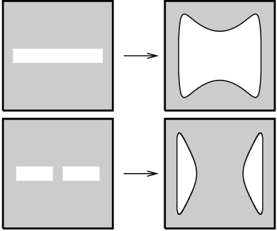
Figure 2: Schematic mapping illustrating conformal transformation of the cuts supporting the eigenvalue distribution visible at figure 1 onto the boundaries of islands for complex eigenvalue distribution. The shaded regions represent holomorphic domain, where the mapping is valid.

The result of this mapping (continuous line) is presented on Fig. 3. The dots are the numerically generated eigenvalues of (31). The mapping reproduces immediately results of original random matrix model for $\mu$ [22]. The islands reproduce the domains of mixed-quark condensate (“phony vacua”), obtained as an artifact of neglecting in the process of averaging the phase of the complex fermion determinant. This condensate is not the usual chiral quark condensate, but quark-conjugate quark condensate which forms due to the fact that quenching of the phase stops penalizing attraction leading to such configurations. Such a condensate violates spontaneously baryon number. This model suggests the reasons for failure of the quenched lattice calculations with chemical potential, due to the appearance of this mixed-condensate or, equivalently, infinitely growing fluctuations when approaching the boundaries of the islands [23], due to the appearance of so-called “baryonic pion”.

Figure 3: Comparison of the numerically obtained distribution of eigenvalues for few sample chemical potentials with analytical results. The solid lines represent the boundaries obtained by conformal mapping.

2.8 Chemical potential - ordinary vacua

We may also consider the random model without suppressing the phase of the determinant. The investigation of the behavior of unquenched partition function (e.g. location and densities of Lee-Yang zeroes [24]) could be immediately inferred from integration of Blue’s functions. The location of singularities separating the “phases” of the system may be found from equating the real parts of the free energies calculated for different solutions (labeled $(i,j)$) of the cubic Pastur-Wegner equation (32). Explicitly, the location of singularities of partition function for model (31) is given by

$${\rm Re}F_{i}={\rm Re}(G_{i}^{2}+\log\frac{z-G_{i}}{G_{i}})={\rm Re}(G_{j}^{2}+\log\frac{z-G_{j}}{G_{j}})={\rm Re}F_{j}$$ (34)

This procedure describes very nicely precise (up to 500 digit accuracy) numerical calculations of [25]. The resulting phase structure suggests first order phase transition, as discussed in [10].

2.9 Phase diagram

The combination of temperature and chemical potential can be easily investigated as discussed in subsection 2.4. The $1/N$ approximation is reminiscent of the mean-field treatment discussed originally in [10]. The phase diagram (for chiral case) for condensate is plotted on Fig. 4. For chemical potential $\mu>\mu_{crit}=1/6\Sigma\ln(2+\sqrt{3})$ the transition is first order (due to lack of vector couplings in 0d NJL model) and disappears at $\mu=0.5\Sigma$. At zero chemical potential, the transition is second order (mean-field) with critical temperature $T_{crit}=1/4\Sigma$. The different numerical coefficient comparing to subsection 2.4 stems from the fact, that here we have taken into account all Matsubara modes.

Figure 4: Condensate vs temperature and chemical potential for chiral random matrix model with infinitely many Matsubara frequencies included.

It is interesting to compare Fig. 4, obtained using only the constant modes, to the full NJL result of Weise and Lutz [26] and also Zhuang et al. [27]

2.10 U(1) problem

Let us now look at more subtle applications of random matrix models, where usual mean field arguments do not hold and the dynamical effects of fermionic determinant have to be taken into account. We start from the $U(1)$ problem, i.e. the fact that pseudoscalar boson is much heavier than other pseudoscalars, violating bounds based on chiral symmetry. This problem is related to axial anomaly. In subsection 3 we have encounter the “kinematical version” of Atiyah-Singer theorem. Since in QCD Atiyah-Singer theorem is nothing but the global (integrated) axial anomaly, we may hope that the effects of fluctuations in $(n_{R}-n_{L})$, leading to chirality-odd spectral density, may mimic some features of anomalous sector of QCD.

Naively, it looks that the effects of asymmetry $x$ are meaningless in the large $N$ limit. Variable $x=(n_{R}-n_{L})/2N$ seems to be irrelevant in the large $N$ limit. This reasoning is false, due to the fact, that the subleading at the first glance terms coming from asymmetry are enhanced by factor $N$ coming from fermionic loops. The resolution of this problem requires therefore an infinite resummation of contributions originating from fermion determinant.

Technically, we could do it in one step using the integration of the Blue’s (see Appendix). For a fixed asymmetry $x\equiv\chi/2N$ we have

$$\partial_{z}\log Z(\chi)=-2NN_{f}i{\rm Tr}G$$ (35)

where ${\rm Tr}G$ is given by first relation in (17). When integrating Blue’s or Green’s functions we need only to study the contribution of order $x^{2}$ from Green’s function, therefore $G(z)\approx-x^{2}/(z^{2}\sqrt{z^{2}-4})$. Straightforward integration leads to

$$[\log Z(\chi)]_{2}=\frac{1}{2N}N_{f}\frac{1}{m(\sqrt{m^{4}+4}+m)}\chi^{2}$$ (36)

where index reflects the approximation and the constant was fixed from imposing the right asymptotic behavior. Full partition function is

$$Z=\int d\chi e^{\frac{-\chi^{2}}{2\chi^{*}N}}Z(\chi)$$ (37)

where integration over $\chi$ takes into account the fluctuations in number of right-handed and left handed zero modes. The Gaussian measure is consistent with axial anomaly [28].

Inserting (36) into above equation leads to replacement

$$1/\chi^{*}\rightarrow 1/\tilde{\chi}^{*}=1/\chi^{*}+\!\sum_{i=1}^{N_{f}}\frac{1}{m_{f}(\sqrt{m_{f}^{4}\!+\!4}\!+\!m_{f}})\equiv 1/\chi^{*}\!+\!\sum_{i=1}^{N_{f}}\gamma_{i}$$ (38)

where we have used the shorter notation and we have reinstated more general (unequal flavors) flavor dependence.

Note that for $N_{f}=0$ (quenched) the topological susceptibility is just the given by $\chi^{*}$, as it should, reminding the Witten-Veneziano relation known from QCD without light flavors. The unquenched result $\tilde{\chi}^{*}$ shows the screening caused by fermion determinant (quark loops) and vanishes in the chiral limit, in agreement with the theorems of the QCD. The formal trick with the integration of the Blue’s functions allowed us to resum infinitely many infrared terms, and obtained a strictly non-perturbative result. “Quark loops” (terms of order $x^{2}$) from fermion determinant were absolutely crucial for this resummation, since quenched result does not lead to the screening. The presented result is the analog of the screening phenomenon in a statistical ensemble made of negative and positive topological charges in full (unquenched) QCD. Similar mechanism works in the instanton vacuum [29].

2.11 Pseudoscalar susceptibility

Let us finally demonstrate that the manifestations of the U(1) anomaly are identical in QCD and our random matrix model, leading to the same generic screening of pseudoscalar susceptibility. We note that the RMM leads to “Ward identity” relating topological susceptibility, pseudoscalar susceptibility and condensate

$$\tilde{\chi}=-\frac{2m}{N_{f}^{2}}i{\rm TrG}-\frac{m^{2}}{N_{f}^{2}}\chi_{ps},$$ (39)

in analogy to anomalous Ward identity in Minkowski QCD

$$i\chi_{top}=-\frac{im}{N^{2}_{f}}\langle{\bar{\psi}\psi}\rangle+\frac{m^{2}}{N^{2}_{f}}\int d^{4}x\langle{T^{*}\bar{\psi}i\gamma_{5}\psi(x)\bar{\psi}i\gamma_{5}\psi(0)}\rangle$$ (40)

where the pseudoscalar susceptibility is defined by the integral in (40). The resolution of the U(1) problem in QCD stems from the fact that for small chiral mass $m$, the absence of the U(1) Goldstone boson requires that $\chi_{top}=-m\langle{\bar{\psi}\psi}\rangle/N_{f}^{2}$ to order ${\cal O}(m^{2})$, or in other words, pseudoscalar susceptibility has to be finite in the chiral limit. In random matrix model, the above unquenched calculations and Ward identity yield the pseudoscalar susceptibility to be equal [30]

$$\chi_{ps} \equiv \frac{1}{N}[-\langle{{\rm tr}{\bf Q}^{-1}\gamma_{5}{\bf Q}^{-1}\gamma_{5}}\rangle+\frac{1}{N}\langle{{\rm tr}{\bf Q}^{-1}\gamma_{5}{\rm tr}{\bf Q}^{-1}\gamma_{5}}\rangle_{connected}$$ (41)

$$\sim (\sum_{i}^{N_{f}}\frac{1}{m_{i}})^{2}\cdot\frac{1}{1/\chi^{*}+\sum_{i}^{N_{f}}\gamma_{i}}-4\sum_{i}^{N_{f}}\gamma_{i}$$

therefore finite in the chiral limit. The first equality is the definition of pseudoscalar susceptibility in chiral random model. The second equality is the result of our calculations. Note the non-trivial cancellation of the infrared singularities $1/m^{2}$ between the two terms in (41). This remarkable cancellation is the result of competition between the trace and trace-trace terms in (41). Naive expectation based upon large N counting suggests wrongly that the trace-trace term is subleading. Neglecting the trace-trace term leads to diverging pseudoscalar susceptibility in the chiral limit, therefore to the “Goldstone pole” in U(1) channel, and consequently to the failure of the resolution of the anomaly problem. Like in real QCD, the unquenched treatment of large oscillations (${\cal O}(N^{1/2})$ , where N commensurates with volume) in topological charge are needed for proper physics in the U(1) channel. We found rather remarkable that the simple matrix model without any further dynamical assumptions is able to illustrate the mechanism of screening consistent with our knowledge of the QCD. We do hope also that some of these results are relevant for lattice simulation for U(1) observables, taking into account that the resummation of infrared terms might be troublesome on the finite lattice.

2.12 Finite $\theta$

QCD at finite vacuum angle $\theta$ is not well understood. Despite experimental evidence suggest that $\theta<10^{-10}$, the issue of potential CP breakdown of QCD poses a serious theoretical challenge. Since due to the U(1) anomaly, the $\theta$ term may be traded from gauge fields to the quark mass matrix, some problems of $\theta$ term may be investigated using the chiral random matrix models, provided that the mass matrix ${\rm diag}\,(m_{1},m_{2},...m_{N_{f}})$ is replaced by $e^{i\theta/N_{f}}{\rm diag}\,(m_{1},m_{2},...m_{N_{f}})$.

Saddle point analysis [31] leads to the following unsubtracted free energy (for small masses)

$$F = \sum_{j=1}^{N_{f}}\left(p_{j}^{2}-\log{p_{j}^{2}}-2\frac{m_{j}}{p_{j}}\cos{\phi_{j}}\right)$$

$$+ \frac{\chi_{*}V}{2N}\left(\theta-\sum_{j=1}^{N_{f}}\phi_{j}-\sum_{j=1}^{N_{f}}\frac{m_{j}}{p_{j}}\sin\phi_{j}\right)^{2}+O(m_{j}^{2})$$

where saddle point solutions of RMM are parameterized as $p_{j}e^{i(\theta/N_{f}-\phi_{j})}$. Remarkably, this RMM result reproduces Witten equations [32], derived using different arguments. For $N_{f}=3$ the solution at $\theta=\pi$ is doubly degenerated, implying spontaneous breakdown of CP, provided the Dashen bound holds. For physical masses, however, spontaneous breakdown of CP seems to be excluded.

Encouraged by these analytical results, we may probe numerically the unquenched $\theta$ problem in the framework of random matrix models. At the left side of Fig. 5 we plot the numerical results [31] for free energy as a function of vacuum angle. On the right side, we compare the similar plot from [33], obtained for dynamical $CP^{3}$ model (plots for QCD do not exist due to the complexity of the problem). Both plots exhibit a kink at some critical value, suggesting first order “deconfining” phase transition. If this transition would persist for QCD, such picture may suggest a dynamical resolution of the $\theta$ problem. Namely, deconfinement may always happen due to the fact that chromomagnetic monopoles would acquire electric charges $\theta/2\pi$, and would screen in consequence long-range color forces. Therefore the presence of confining phase forces $\theta=0$.

Such scenario requires that the kink visible on both figures migrates to zero in the thermodynamical limit.

   

Figure 5: Free energy as a function of $\theta/\pi$ for RMM (left) and $CP^{3}$ model [33]. Here $\lambda=N/V$.

RMM allows another scenario consistent with the CP³ data. High precision numerical studies in RMM [31] strongly suggest that the major factor driving the position of the kink seems to be rather the ratio $N/V$, where $N$ refers to number of zero modes in a fixed volume $V$. Therefore the kink observed for dynamical models like $CP^{3}$ may be the result of subtle interplay between quark masses, finite size effects and accuracy in numerical assessments.

3 CONCLUSIONS

In this talk, we tried to give a quick overview of applications of RMM to various domains of QCD, with the emphasis on the phenomenon of spontaneous breakdown of chiral symmetry. The main intention of this presentation was to exhibit the generic behavior based on fundamental physical premises. We therefore have skipped several important technical details and we have often referred to original papers. Meanwhile, we tried to stress the fact, that several “miraculous” at the first glance agreements of RMM and QCD, either at quantitative level (microscopic regime) or at qualitative level (macroscopic regime), are based on firm and well understood principles of spontaneous breakdown of chiral symmetry.

We do hope that this way of looking at RMM in reference to QCD may be helpful at least for a non-expert in Random Matrix Models.

APPENDIX - FIVE FACETS OF BLUE’S

The fundamental problem in random matrix theories is to find the distribution of eigenvalues in the large $N$ (size of the matrix ${\cal M}$) limit [34]. One encounters two generic situations — in the case of hermitian matrices the eigenvalues lie on one or more intervals on the real axis, while for general non-hermitian ones, the eigenvalues occupy two-dimensional domains in the complex plane. In both cases the distribution of eigenvalues can be reconstructed from the knowledge of the Green’s function:

$$G(z)=\frac{1}{N}\left<{\rm tr}\frac{1}{z-{\cal M}}\right>$$ (43)

where averaging is done over the ensemble of $N\times N$ random matrices generated with probability

$$P({\cal M})=\frac{1}{Z}e^{-N{\rm tr}V({\cal M})}$$ (44)

For hermitian matrices the discontinuities of the Green’s function coincide with the eigenvalue supports. In the simplest example of the Gaussian potential $V({\cal M})={\cal M}^{2}$ for hermitian matrix ${\cal M}$, a standard calculation gives

$$G(z)=\frac{1}{2}(z-\sqrt{z^{2}-4})$$ (45)

The reconstruction of the spectral function (i.e. eigenvalue distribution) is based on the well known relation

$$\frac{1}{x\pm i\epsilon}={\rm PV}\frac{1}{x}\mp i\pi\delta(x)$$ (46)

Then, the spectral function turns out to be

$$\nu(\lambda)=-\frac{1}{\pi}\lim_{\epsilon\rightarrow 0}{\rm Im}G(z)|_{z=\lambda+i\epsilon}$$ (47)

In the case of the Gaussian Green’s function (45), the discontinuities in the Green’s function come from the cut of the square root, leading to the Wigner’s semicircle law $\nu(\lambda)=\frac{1}{2\pi}\sqrt{4-\lambda^{2}}$ for the eigenvalue distribution of random hermitian matrices.

The Blue’s function is defined as a functional inverse of the Green’s function

$$B[G(z)]=z$$ (48)

For random Gaussian ensemble, the functional inverse of (45) is simply $B(z)=z+1/z$. Blue’s functions were introduced by Zee [1] as the result of diagrammatic reinterpretation of the seminal addition formalism (R-transformation) by Voiculescu [2].

3.1 Addition

Let us consider the problem of calculating Green’s function for the sum of two independent ensembles ${\cal M}_{1}$ and ${\cal M}_{2}$, i.e.

$$G(z) = \frac{1}{N}\int[d{\cal M}_{1}][d{\cal M}_{2}]P({\cal M}_{1})P({\cal M}_{2}){\rm tr}\frac{1}{z-{\cal M}_{1}-{\cal M}_{2}}$$

$$\equiv \frac{1}{N}\left<{\rm tr}\frac{1}{z-{\cal M}_{1}-{\cal M}_{2}}\right>$$

The concept of addition law for hermitian ensembles relies on additive transformation, which linearizes the convolution of non-commutative matrices (3.1), alike to the logarithm of the Fourier transformation for the convolution of arbitrary functions. This method is an important shortcut to obtain the equations for the Green’s functions for a sum of matrices, starting from the knowledge of the Green’s functions of individual ensembles of matrices.

The addition law for Blue’s functions reads [1]

$$B_{1+2}(z)=B_{1}(z)+B_{2}(z)-\frac{1}{z}.$$ (50)

Using the definition of the Blue’s function we could rewrite the last equation in the “operational” form

$$z=B_{1}(G)+B_{2}(G)-G^{-1}$$ (51)

with $G_{1+2}\equiv G$. The algorithm of addition is now surprisingly simple [1]: Knowing $G_{1}$ and $G_{2}$, we find (48) $B_{1}$ and $B_{2}$. Then we read out from (51) the final equation for the resolvent for the sum. Note that the method treats on equal footing the Gaussian and non-Gaussian ensembles, provided that the ensembles are sufficiently independent (free). It is also applicable for chiral random matrices. For generalization of this algorithm for the case arbitrary complex random matrices we refer to original papers [35, 36, 37].

3.2 Multiplication

Blue’s functions provide also an important shortcut to obtain the equation for the Green’s (Blue’s) function for a product of matrices, starting from knowledge of Green’s (Blue’s) functions of individual ensembles of matrices, i.e. to find

$$G(z)=\frac{1}{N}\left<{\rm tr}\frac{1}{z-{\cal M}_{1}\cdot{\cal M}_{2}}\right>$$ (52)

provided that ${\cal M}_{1}$ and ${\cal M}_{2}$ are free and $\langle{{\rm tr}{\cal M}_{1}}\rangle,\langle{{\rm tr}{\cal M}_{2}}\rangle\neq 0$. Introducing the notation for continued fraction

$$\frac{w}{\Sigma_{{\cal M}}\left(\frac{w}{\Sigma_{{\cal M}}\left(\frac{w}{\Sigma_{{\cal M}}(...)}\right)}\right)}\equiv\frac{w}{\Sigma_{{\cal M}}(\bullet)}$$ (53)

where self-energy $\Sigma(z)$ is defined in a standard way $1/G(z)=z-\Sigma(z)$ multiplication law for Blue’s functions reads[38]

$$B_{1\star 2}\left(\frac{w}{\Sigma_{1\star 2}(\bullet)}\right)=\frac{w}{1+w}B_{1}\left(\frac{w}{\Sigma_{1}(\bullet)}\right)\cdot B_{2}\left(\frac{w}{\Sigma_{2}(\bullet)}\right)$$ (54)

The usage of Blue’s functions provides the factorization mechanism for averaging procedure in (52) and is equivalent to S transformation of Voiculescu via [38]

$$S(w)=\frac{1}{\Sigma\left(\frac{w}{\Sigma(\bullet)}\right)}$$ (55)

where $S(w)=\chi(w)(1+1/w)$ with $\chi(zG(z)-1)=1/z$.

3.3 Differentiation

As demonstrated by Zee, differentiation of the Blue’s function leads to determination of the endpoints of the eigenvalue distribution for hermitian random matrices. One could easily visualize this point recalling the form of the Green’s function for Gaussian distribution (45). When approaching the endpoints $z=\pm 2$, the imaginary part of Green’s function vanishes like $\sqrt{(2-\lambda)(2+\lambda)}$. Therefore, the endpoints fulfill the equation $G^{\prime}(z)|_{z=\pm 2}=\infty$, which may be used as the defining equation for unknown endpoints in case of more complicated ensembles. Since Blue’s function is the functional inverse of the Green’s function, the location of the endpoints could be inferred from a simpler relation [1]

$$\frac{dB(G)}{dG}=0$$ (56)

3.4 Integration

Let us consider the partition function depending on a parameter $z$:

$$Z_{N}=\langle{\det(z-{\cal M})}\rangle$$ (57)

For finite $N$ the partition function is a polynomial in $z$ and has $N$ zeroes (Yang-Lee zeroes):

$$Z_{N}=(z-z_{1})(z-z_{2})\dots(z-z_{N})$$ (58)

Taking the logarithm and approximating the density of zeroes by a continuous distribution we get

$$\log\left<{\det(z-{\cal M})}\right>=\sum_{i}\log(z-z_{i})=\int\rho(z^{\prime})\log(z-z^{\prime})dz^{\prime}$$ (59)

We see that the density of Yang-Lee zeroes can be reconstructed from the discontinuities of the unquenched Green’s function:

$$\partial_{z}\log\left<{\det(z-{\cal M})}\right>=\left<{\mbox{\rm tr}\,\frac{1}{z-{\cal M}}\cdot\det(z-{\cal M})}\right>$$ (60)

using e.g. Gauss law  [39]. For $z$ close to infinity the unquenched and quenched (43) Green’s functions coincide. Moreover the unquenched resolvent is nonsingular configuration by configuration and hence is holomorphic. Therefore it is exactly the functional inverse of the ordinary hermitian Blue’s function. In general we may have several branches of Green’s functions, which are determined by different saddle points contributing to (57). The discontinuity (cusp) and hence the location of Yang-Lee zeroes is determined by the possible contribution of two of them. From a $1/N$ expansion

$$\log Z_{N}=NF_{0}+F_{1}+\frac{1}{N}F_{2}+\ldots$$ (61)

we see that two saddle points may contribute if

$${\rm Re}F_{0}^{sp.I}={\rm Re}F_{0}^{sp.II}$$ (62)

and $F_{0}$ is determined by (60)

$$F_{0}=\int^{z}dz^{\prime}G(z^{\prime})+const$$ (63)

or equivalently

$$E_{0}=zG-\int\!dG\ B(G)+const$$ (64)

after integrating by parts. Note that we have used the fact that $z(G)=B(G)$ is just the Blue’s function [1] of $G$, The integration using Blue’s function is in most cases much simpler than the corresponding direct integration of $G(z)$.

3.5 Mapping

In case of non-hermitian random matrices, eigenvalues are complex. The average density of eigenvalues follows from the electrostatic analogy to two-dimensional Gauss law

$$\nu(z,\bar{z})=\frac{1}{\pi}\partial_{\bar{z}}G(z,\bar{z})$$ (65)

Contrary to hermitian case, when eigenvalues condense on cuts, here they form two-dimensional nonholomorphic (non-analytic) “islands”. Surprisingly, using only the analytical structure of the Blue’s functions, we can find the boundaries of these “islands”, while staying wholly within the holomorphic region [40].

Let us consider an example. First, we consider the case where a Gaussian random and hermitian matrix $H$ is added to an arbitrary hermitian matrix $M$, then the case where a Gaussian random and anti-hermitian matrix $iH$ is added to the same matrix $M$. In first case, eigenvalues are on the cuts (they are real), in the second case, form an island. In both cases the regions free of eigenvalues are holomorphic (here fulfill the Laplace equation). This implies that there exists a conformal transformation relating these two domains of analyticity. For the case considered here, Blue’s functions for both cases are related via

$$B_{iH+M}(u)=B_{H+M}(u)-2u$$ (66)

Substituting $u\rightarrow G_{H+M}(z)$ we can rewrite (66) as

$$B_{iH+M}[G_{H+M}(z)]=z-2G_{H+M}(z)\,.$$ (67)

Let $w$ be a point in the complex plane for which $G_{iH+M}(w)=G_{H+M}(z)$. Then, using the definition of the Blue’s function, we get

$$w=z-2G_{H+M}(z)\,.$$ (68)

Equation (68) provides a conformal transformation mapping the holomorphic domain of the ensemble $H+M$ (i.e. the complex plane $z$ minus cuts) onto the holomorphic domains of the ensemble $iH+M$, i.e. the complex plane $w$ minus the “islands”, defining in this way the support of the eigenvalues. Such construction could be generalized for other non-gaussian ensembles, due to the fact that addition of Blue’s functions forms an abelian group.

References

References

- [1] A. Zee, Nucl. Phys. B474, 726 (1996).
- [2] D.V. Voiculescu, Invent. Math. 104, 201 (1991); D.V. Voiculescu, K.J. Dykema and A. Nica, “Free Random Variables”, Am. Math. Soc., Providence, RI, (1992); for new results see also A. Nica and R. Speicher, Amer. J. Math. 118, 799 (1996) and references therein.
- [3] T. Banks and A. Casher, Nucl. Phys. B169, 103 (1980).
- [4] R.A. Janik, M.A. Nowak, G. Papp and I. Zahed, e-print hep-ph/9803289.
- [5] for recent reviews, see T. Schäfer, E.V. Shuryak, Rev. Mod. Phys. 70, (1998) 323; D. Diakonov, e-print hep-ph/9602375.
- [6] S. Weinberg, Physica 96A, 327 (1979); J. Gasser and H. Leytwyler, Ann. Phys. 158, 142 (1984).
- [7] J. Gasser and H. Leutwyler, Phys. Lett. B184, 142 (1987); ibid. B188, 477 (1987); Nucl. Phys. B307, 763 (1988).
- [8] H. Leutwyler and A. Smilga, Phys. Rev. D46, 5607 (1992).
- [9] E.V. Shuryak and J.J.M. Verbaarschot, Nucl. Phys. A560, 306 (1993).
- [10] M.A. Nowak, M. Rho and I. Zahed, Chiral Nuclear Dynamics, World Scientific, Singapore, 1996.
- [11] J.J.M. Verbaarschot and I. Zahed, Phys. Rev. Lett. 70, 3852 (1993).
- [12] G. Akemann, P.H. Damgaard, U. Magnea and S. Nishigaki, Nucl. Phys. B487, 721 (1997).
- [13] J.J.M. Verbaarschot, Acta Phys. Polon. B25, 133 (1994).
- [14] T. Wettig, T. Gühr, A. Schäfer and H.A. Weidenmüller, Hirschegg Lectures (1997), e-print hep-ph/9701387; M.E. Berbenni-Bitsch et al., e-print hep-lat/9704018.
- [15] R. Pisarski and F. Wilczek, Phys. Rev. D29, 338 (1984).
- [16] A.D. Jackson, M.K. Sener and J.J.M. Verbaarschot, Nucl. Phys. B479, 707 (1996).
- [17] J. Jurkiewicz, M. A. Nowak and I. Zahed, Nucl. Phys. B478, 605 (1996); Erratum -ibid. B513, 759 (1998).
- [18] P.H. Damgaard and S.M. Nishigaki, Nucl. Phys. B518, (1998) 495; T. Wilke, T. Guhr and T. Wettig, Phys. Rev. D57, (1998) 6486.
- [19] E.P. Wigner, Proc. Camb. Phi. Soc. 47, 790 (1951).
- [20] A.D. Jackson and J.J.M Verbaarschot, Phys. Rev. D53, 7223 (1996).
- [21] L.A. Pastur, Theor. Mat. Phys. (USSR) 10, 67 (1972); F. Wegner, Phys. Rev. B19, 783 (1979).
- [22] M. Stephanov, Phys. Rev. Lett. 76, 4472 (1996); M. Stephanov, Nucl. Phys. Proc. Suppl. 53, 469 (1997).
- [23] R.A. Janik, M.A. Nowak, G. Papp and I. Zahed, Phys. Rev. Lett. 77, 4876 (1996).
- [24] for a review, see e.g. K. Huang, Statistical Mechanics, John Wiley, New York (1987).
- [25] A. Halasz, A.D. Jackson and J.J.M. Verbaarschot, Phys. Lett. B395, 293 (1997); A. Halasz, A.D. Jackson and J.J.M. Verbaarschot, Phys. Rev. D56, 5140 (1997).
- [26] U. Vogel and W. Weise, Prog. Part. and Nucl. Phys. 27, 195 (1991).
- [27] P. Zhuang, J. Hüfner and S.P. Klevansky, Nucl. Phys. A576, (1994) 525.
- [28] R. Alkofer, M.A. Nowak, J.J.M. Verbaarschot and I. Zahed, Phys. Lett. B233, 205 (1989).
- [29] D. Diakonov, M.V. Polyakov and C. Weiss, Nucl. Phys.B461, 539 (1996).
- [30] R.A. Janik, M.A. Nowak, G. Papp and I. Zahed, Nucl. Phys. B498, 313 (1997).
- [31] R.A. Janik, M.A. Nowak, G. Papp and I. Zahed, to be published.
- [32] E. Witten, Ann. Phys. 128, 363 (1980).
- [33] G. Schierholz, Nucl. Phys. Proc. Suppl. A37, (1994) 203.
- [34] For an excellent recent review, see T. Guhr, A. Müller-Gröling and H.A. Weidenmüller, Phys. Rept. 299, (1998) 189.
- [35] R.A. Janik, M.A. Nowak, G. Papp and I. Zahed, Nucl. Phys. B501, 603 (1997).
- [36] J. Feinberg and A. Zee, Nucl. Phys. B501, 643 (1997).
- [37] R.A. Janik, M.A. Nowak, G. Papp and I. Zahed, Acta Phys. Polon. B28, 2949 (1997).
- [38] R.A. Janik, Ph.D. Thesis, Cracow 1997 (unpublished).
- [39] J. Vink, Nucl. Phys. B323, 399 (1989)
- [40] R.A. Janik, M.A. Nowak, G. Papp, J. Wambach and I. Zahed, Phys. Rev. E55, 4100 (1997).