Entanglement of Fock-space expansion and covariance in light-front Hamiltonian dynamics^∗

Abstract

We investigate in a model with scalar “nucleons” and mesons the contributions of higher Fock states that are neglected in the ladder approximation of the Lippmann-Schwinger equation. This leads to a breaking of covariance, both in light-front and in instant-form Hamiltonian dynamics. The lowest Fock sector neglected has two mesons in the intermediate state and corresponds to the stretched box. First we show in a simplified example that the contributions of higher Fock states are much smaller on the light-front than in instant-form dynamics. Then we show for a scattering amplitude above threshold that the stretched boxes are small, however, necessary to retain covariance. For an off energy-shell amplitude covariance is not necessarily maintained and this is confirmed by our calculations. Again, the stretched boxes are found to be small.

]

I Introduction

In his famous article of 1949, Dirac [1] described a number of ways how to set up a framework of Hamiltonian dynamics. Two of these are most important. In instant-form (IF) Hamiltonian dynamics one specifies the initial conditions on the equal-time plane $t=0$. Of the ten Poincaré generators six are kinematic, i.e., do not contain interactions, and are therefore conserved quantities, and four are dynamical: the three boost operators and the energy. In light-front (LF) Hamiltonian dynamics one uses the coordinates

$$A^{\perp}=(A^{x},A^{y}),\quad A^{\pm}=\frac{A^{0}\pm A^{z}}{\sqrt{2}},$$ (1)

and quantizes on the plane $x^{+}=0$. Then only three operators are dynamical. Two of them involve rotations around the $x$ or $y$-axis. Therefore LF time-ordered amplitudes are not invariant under such rotations.

The question of rotations in LF dynamics (LFD) was discussed before with the aim of constructing the angular momentum operators, see e.g. Fuda [2], and the review by Carbonell et al. [3]. While these authors emphasize the algebraic properties of the generators of the Poincaré group, we stress in the present paper the connection between expansions in Fock-space and covariance. It has been remarked before by Brodsky et al. [4] that the higher components in Fock space contribute to the difference between the Bethe-Salpeter equation and the evolution equation in LFD. These authors do not give numerical estimates of the corrections. The latter has been done by Mangin-Brinet and Carbonell [5], and by Frederico et al. [6], who studied the same model and found the effect of higher Fock states on the binding energy to be small. In a calculation of positronium, Trittmann and Pauli [7] used an effective theory, where the effects of all Fock states are included in the interaction. They found rotational symmetry to be restored in the solution.

In this paper we consider first standard LF quantization and discuss the problem of noncovariance, which includes violation of rotational invariance, in the framework of LF time-ordered perturbation theory. We give numerical results for the simplified case of two heavy scalars exchanging light scalar particles. This choice is motivated by the popular meson-exchange models in nuclear physics. We do not include the internal spin degrees of freedom, as this is a complication that may obscure the main point of our investigation: the connection between the breaking of covariance and a truncation of the expansion in Fock space. In two interesting papers, Fuda [8, 9] reported on detailed calculations of realistic one-meson exchange models in both LF and IF dynamics. There the emphasis is on the comparison between the two, when in both cases the ladder approximation is made. It is the purpose of the present paper to show to what extent the ladder approximation violates covariance.

A Suppression of higher Fock states

A reason why LFD is preferred by many is that higher Fock states are said to be more strongly suppressed in this form of dynamics. As a disadvantage the lack of manifest rotational invariance, and therefore covariance, is mentioned. We call a symmetry manifest when it is connected to a kinematical operator. Then all time-ordered diagrams exhibit this symmetry. Equal-time ordered diagrams lack boost invariance whereas on the LF the longitudinal boost $P^{+}$ is a kinematical operator. Therefore, if one complains about lack of manifest covariance, one should include not only rotational invariance but also other nonmanifest symmetries. One reason why people have rather stressed rotational invariance comes easily to mind: in many cases it is easy to convince oneself by inspection whether a matrix element is rotational invariant, viz when the amplitude can be expressed in terms of scalar products of three-vectors. On the other hand, it is not more difficult to test numerically for invariance under boost transformations than for invariance under rotations. Indeed, the method used in the present paper can easily be extended to check for boost invariance.

A way to test for covariance is to compare the LF time-ordered diagrams to the covariant amplitude, since we know that the latter is invariant under any of the Poincaré symmetry operations. For on energy-shell amplitudes ($S$-matrix elements) there is an exact equality, as was proved by Ligterink and Bakker [10] and which is confirmed in our results. Off energy-shell there is a deviation, which, however, is found in the present paper to be surprisingly small.

So why are we using these LF time-ordered diagram in the first place, when there is an equivalent covariant method available? We do, because we want to determine the properties of the bound state using the Hamiltonian form of dynamics. In this method, covariance can never be fully maintained. However, one may try to apply it in such a way that breaking of covariance is minimal. In many applications in nuclear physics a one-meson exchange approximation is made for the interaction and the scattering amplitude is computed by formally iterating this interaction, leading to the Lippmann-Schwinger equation in the ladder approximation. In this approximation one retains two- and three-particle intermediate state and neglects Fock states containing four or more particles. These Fock sectors are needed to make the sum of LF time-ordered diagrams equal to the covariant amplitude, exhibiting the symmetries under all Poincaré transformations. If these contributions are large, one can expect a significant breaking of covariance, since the LF time-ordered diagrams are only invariant under application of the kinematical symmetries.

For this reason we concentrate in this article on the determination of the contributions of these higher Fock states. Our main concern shall be the box diagram. Then we label the correction as ${\cal R}_{4^{+}}$. We shall calculate ${\cal R}_{4^{+}}$ explicitly for the box diagram with scalar particles of different masses. The box diagram can be associated with the two-meson exchange between two nucleons. If spin would be included several well-known complications would arise, the most important one being the occurrence of instantaneous propagators [10, 11]. We do not want these complications to interfere with the main point of our investigation: the connection between Fock-space truncations and lack of covariance. Therefore spin is omitted. We have not included crossed box diagrams, because they are not relevant for a discussion on covariance, since both the crossed and noncrossed box diagram are covariant by themselves.

B Setup

First we explain the Lippmann-Schwinger formalism and the special role of the box diagram. In Sec. III we describe how to calculate both the covariant and the LF time-ordered amplitudes. After this, we are ready for our numerical experiments. In Sec. V the masses of the external particles are chosen in such a way that on-shell singularities of the intermediate states are avoided, and therefore it is easy to compare IF and LF Hamiltonian dynamics. In that section it is shown that ${\cal R}_{4^{+}}$ is much smaller in LFD than in IF dynamics (IFD), confirming the claim that in LFD higher Fock states are more strongly suppressed. Moreover, it tells us that covariance is more vulnerable in IFD than on the light-front!

After this exercise, we concentrate on the LF, and in Sec. VI we calculate the LF time-ordered diagrams for the more interesting case in which we have particles of fixed masses $m$ (called nucleons) and $\mu$ (called mesons). As the process we are concerned with, scattering, is above threshold, we have to deal with on-shell singularities. We show that the breaking of covariance is again small.

Although in Sec. VII, where we discuss off-shell amplitudes below threshold, no on-shell singularities are encountered, matters become more complicated because the notion of the c.m. frame becomes ambiguous, since the total momentum $P^{z}$ is dynamical and found to be unequal to the combined momentum of the two particles, $p^{z}+q^{z}$. However, we are still able to relate the breaking of covariance and Fock-space truncation.

The lack covariance of the LF time-ordered amplitudes means that the amplitude depends not only on the scalar products of the external momenta, but on the angles between the quantization axis and the external momenta as well. Consequently, the amplitudes must have singularities as a function of these angles in addition to the familiar singularities as functions of the invariants. The positions of these singularities are found analytically in Sec. VIII, in the framework of explicitly covariant LFD. This gives a qualitative understanding of the numerical results in Secs. V and VI. In Sec. IX explicitly covariant LFD is applied to the off energy-shell results of Sec. VII.

II The Lippmann-Schwinger formalism

The Hamiltonian method aims at the determination of stationary states, i.e. eigenstates of the Hamiltonian. Here we take the Yukawa-type model with scalar coupling

$${\cal L}_{\rm int}=g\Phi^{2}\phi.$$ (2)

Two types of particles are considered: “nucleons” (N, $\Phi$) with mass $m$ and “mesons” (m, $\phi$) with mass $\mu$. The Hamiltonian $H\equiv P^{-}$ consists of a part $H_{0}$ which describes free particles and a part $V$ which describes the interaction:

$$H=H_{0}+V.$$ (3)

We shall denote the second term on the r.h.s. as the potential. The problem of constructing the Hamiltonian from the underlying Lagrangian has been recently reviewed by Brodsky et al. [12]. Here we study two-nucleon states only. Moreover, we neglect self-energy diagrams.

We consider $H_{0}$, the kinematic part of the Hamiltonian in the two-nucleon (2N) sector. In the instant-form, quantization is carried out on planes of constant time (equal-time planes). Then we find for two particles of mass $m$ and momenta $p$ and $q$ respectively

$$H_{0}^{\rm IF}=\sqrt{\vec{p}^{2}+m^{2}}+\sqrt{\vec{q}^{2}+m^{2}},$$ (4)

which leads to both negative and positive energy solutions. It is well-known [13] that in this form the overall momenta and the relative momenta are difficult to separate.

In LF quantization the square root, and therefore the negative energy solutions are absent. The interaction-free part of the two-body Hamiltonian is

$$H_{0}^{\rm LF}=\frac{{p^{\perp}}^{2}+m^{2}}{2p^{+}}+\frac{{q^{\perp}}^{2}+m^{2}}{2q^{+}},$$ (5)

which demonstrates that positive energies occur for positive plus-momenta. Moreover, one can easily separate the motion of a many-particle system as a whole from the internal motion of its constituents in the LF case [13].

We shall focus on light-front quantization of our model in which the interaction of the nucleons is due to meson exchange. We write the potential in the form

$$V=V_{1}+V_{2}+V_{3}+\dots$$ (6)

where the subscript denotes the number of mesons simultaneously exchanged. The potentials only contain irreducible diagrams to prevent double counting. $V_{1}$ contains one-meson exchanges only:

$$V_{1}=\raisebox{-12.80365pt}{\epsfbox{oneb.eps}}=\raisebox{-7.11317pt}{\epsfbox{oneba.eps}}+\raisebox{-7.11317pt}{\epsfbox{onebb.eps}}$$ (7)

The irreducible diagrams contributing to $V_{1}$ are depicted in Eq. (7). In these diagrams time goes from left to right. The nucleons are denoted by solid lines, and the mesons by dashed lines. Irreducible diagrams contributing to $V_{2}$ are those diagrams of order $g^{4}$ that cannot be separated into two pieces by cutting two nucleon lines or two nucleon lines and one meson line only. In terms of Fock-space sectors this means that $V_{1}$ contains two-nucleon and one-meson intermediate states, and $V_{2}$ contains only two-nucleon two-meson intermediate states.

The potential $V_{1}$ is a covariant object in the case the external lines are on shell. The meaning of the equal sign in Eq. (7) is that the full covariant amplitude can be written as a sum of two LF time-ordered diagrams. Whereas the Feynman diagram contains the propagator $1/((q^{\prime}-q)^{2}-\mu^{2})$, the LF time-ordered diagrams contain the energy denominator $1/(P^{-}-H_{0})$, $P^{-}$ being the parametric energy. $H_{0}$ is the sum of the kinetic energies of the particles in the intermediate state:

$$H_{0}=\sum_{i}\frac{{k^{\perp}_{i}}^{2}+m^{2}_{i}}{2k^{+}_{i}}.$$ (8)

The two diagrams contain $\theta$-functions of the plus-component of the momentum of the exchanged meson: one has the factor $\theta(p^{+}-q^{+})$, the other $\theta(q^{+}-p^{+})$.

In a Feynman diagram the external lines are on mass shell and the initial and final states have the same energy, which coincides with the parametric energy. Then the minus component of the total four-momentum of a two-particle state satisfies the relation

$$P^{-}=p^{-}+q^{-}=p^{\prime-}+q^{\prime-}=\frac{p^{2}_{\perp}+m^{2}}{2p^{+}}+\frac{q^{2}_{\perp}+m^{2}}{2q^{+}}.$$ (9)

As the minus component of the total momentum is the only dynamical momentum operator, the other three components are conserved in any LF time-ordered diagram. For instance, $P^{+}=p^{+}+q^{+}=p^{\prime+}+q^{\prime+}$. This conservation law is very important in LF quantization. It leads immediately to the spectrum condition: in any intermediate state all massive particles have plus-momenta greater than zero and the sum of the plus-components of the momenta of the particles in that state is equal to the total plus-momentum.

The expansion in Fock space does not coincide with an expansion in powers of the coupling constant. This can easily be seen when one considers an approach closely resembling the Lippmann-Schwinger method. The eigenstates $|\psi>$ of the Hamiltonian

$$H|\psi>=P^{-}|\psi>,$$ (10)

are also solutions of the Lippmann-Schwinger equation

$$|\psi\rangle=|\phi\rangle+\frac{1}{P^{-}-H_{0}}V|\psi\rangle.$$ (11)

The formal solution of this equation is

$$|\psi>=\sum_{i=0}^{\infty}\left(\frac{1}{P^{-}-H_{0}}V\right)^{i}|\phi>.$$ (12)

An equation similar to Eq. (11) exists for the scattering amplitude:

$$\raisebox{-7.11317pt}{\epsfbox{T.eps}}=\raisebox{-7.11317pt}{\epsfbox{V.eps}}+\raisebox{-7.11317pt}{\epsfbox{VT.eps}}$$ (13)

If one substitutes $V_{1}$ for $V$ in these equations one obtains the ladder approximation. This approximation does not generate all diagrams, so one needs to add corrections. At order $g^{4}$ this correction is $V_{2}$:

$$V_{2} = \raisebox{-7.11317pt}{\epsfbox{box0.eps}}+\raisebox{-7.11317pt}{\epsfbox{box6.eps}}$$ (14)

If one takes into account all the contributions to $V$ from Eq. (6) then the full scattering amplitude is

$$\raisebox{-7.11317pt}{\epsfbox{T.eps}}=\raisebox{-7.11317pt}{\epsfbox{oneba.eps}} +$$ (15)

$$+\raisebox{-7.11317pt}{\epsfbox{box2.eps}}+\raisebox{-7.11317pt}{\epsfbox{box1.eps}} + \raisebox{-7.11317pt}{\epsfbox{box3.eps}}+\raisebox{-7.11317pt}{\epsfbox{box4.eps}}$$ (16)

$$+\raisebox{-7.11317pt}{\epsfbox{box0.eps}}+\raisebox{-7.11317pt}{\epsfbox{box6.eps}} + \quad{\cal O}(g^{6}).$$ (17)

In the ladder approximation one only takes $V_{1}$ into account. Effectively, one then describes the full interaction between two nucleons by

$$\raisebox{-7.11317pt}{\epsfbox{T.eps}}=\raisebox{-7.11317pt}{\epsfbox{oneba.eps}} +$$ (18)

$$+\raisebox{-7.11317pt}{\epsfbox{box2.eps}}+\raisebox{-7.11317pt}{\epsfbox{box1.eps}} + \raisebox{-7.11317pt}{\epsfbox{box3.eps}}+\raisebox{-7.11317pt}{\epsfbox{box4.eps}}$$ (19)

$$+ \quad{\cal O}(g^{6}).$$ (20)

In this approximation intermediate states containing more than three particles do not occur. This implies that time-ordered box diagrams with four particles in the intermediate state are neglected, as we can see if we compare the expansions in Eqs. (17) and  (20). As the individual diagrams contributing to $V_{2}$ are not covariant, the sum of box diagrams produced by the ladder approximation is not covariant.

Using equal-time quantization, twenty out of the twenty-four possible time-orderings have intermediate states with more than three particles. On the LF, the spectrum condition kills many of the time-ordered diagrams. There are six nonvanishing diagrams, of which four only contain two and three-particle intermediate states. One concludes that the one-meson exchange kernel neglects the majority of the contributing time-ordered box diagrams in equal-time quantization, whereas on the LF most of the nonvanishing diagrams are taken into account. This does not mean necessarily that in IF dynamics the ladder approximation misses most of the amplitude, since the missing diagrams have smaller magnitudes. The contribution of the missing diagrams needs to be investigated in order to see how much the higher Fock sectors are suppressed.

There is one thing which seems to complicate matters on the LF. The individual LF time-ordered diagrams are not rotational invariant. When a number of them is missing the full amplitude will also lack rotational invariance, as is mentioned often in the literature. This feature does not occur on the equal-time plane, since here rotational invariance is a manifest symmetry. However, in other types of Hamiltonian dynamics other symmetries are nonmanifest. In IF Hamiltonian dynamics, e.g., boost invariance is not manifest. Therefore, we refer to breaking of covariance, which is a general feature of any form of Hamiltonian dynamics, if one truncates the the Fock-space expansion.

We would like to estimate the contribution of the missing diagrams, irrespective of the strength of the coupling. It is not possible to do this in a completely general way, so we perform our numerical calculations for the box diagram only. We assume that our results will be indicative for the higher orders too.

We define the fraction

$${\cal{R}}^{\rm LF}_{4^{+}}=\frac{\epsfbox{box0.eps}+\epsfbox{box6.eps}}{\raisebox{-14.22636pt}{\epsfbox{boxcov.eps}}}.$$ (21)

The subscript 4 indicates that this variable includes all diagrams having at least 4 particles in some intermediate state. For ${\cal{R}}^{\rm IF}_{4^{+}}$ one would have to add the diagrams containg five and six-particle intermediate states in the numerator, as these give nonvanishing contributions in the instant-form. The diagram in the denominator is the covariant diagram.

We shall show that the correction $V_{2}$ is indeed much less important numerically in LFD than in IFD. So the 2N2m-state is in LFD much less important than in IFD. We conjecture that this property of LFD that the Fock-state expansion converges much more rapidly than in IFD persists in higher orders in the coupling constant.

III The box diagram

In the previous section we saw that the lowest level at which breaking of covariance is to be expected is the two-meson exchange diagram, also referred to as the box diagram. Implicitly, in Sec. II we took the particles to be scalars, as we did not include instantaneous terms which are related to spin-$1/2$ particles. Although a bound state of scalar particles is not found in nature, we do not include spin because we want to avoid in this investigation the complications due to instantaneous terms.

We look at the process of two nucleons with momenta $p$ and $q$ respectively, coming in and exchanging two meson of mass $\mu$. The outgoing nucleons have momenta $p^{\prime}$ and $q^{\prime}$. The kinematics is given in Fig. 1.

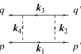
FIG. 1.: Kinematics for the box diagram. The arrows denote the momentum flow.

The internal momenta are

$$k_{1} = k,$$ (22)

$$k_{2} = k-p^{\prime},$$ (23)

$$k_{3} = k-p-q,$$ (24)

$$k_{4} = k-p.$$ (25)

We have to keep in mind that these relations only hold for those components of the momenta that are conserved.

A The covariant box diagram

The covariant box diagram is given by

$$\raisebox{-8.5359pt}{\epsfbox{boxcov.eps}}=\int_{\rm Min}-i\;{\rm d}^{4}k\hskip 56.9055pt$$ (26)

$${\left(({k_{1}}^{2}-m^{2})({k_{2}}^{2}-\mu^{2})({k_{3}}^{2}-m^{2})({k_{4}}^{2}-\mu^{2})\right)^{-1}},$$ (27)

where the subscript “Min” denotes that the integration has a Minkowskian measure. The imaginary parts $i\epsilon$ of the masses have been dropped.

B Equivalence

If the external states are on energy-shell, that is,

$$P^{-}=p^{-}+q^{-}=p^{\prime-}+q^{\prime-},$$ (28)

then the time-ordered diagrams are the same as those derived by integrating the covariant diagram over light-front energy $k^{-}$. In that case we have

$$\raisebox{-8.5359pt}{\epsfbox{boxcov.eps}}=\raisebox{-7.11317pt}{\epsfbox{box1.eps}}+\raisebox{-7.11317pt}{\epsfbox{box3.eps}}+\raisebox{-7.11317pt}{\epsfbox{box2.eps}}$$ (29)

$$+\raisebox{-7.11317pt}{\epsfbox{box4.eps}}+\raisebox{-7.11317pt}{\epsfbox{box0.eps}}+\raisebox{-7.11317pt}{\epsfbox{box6.eps}}$$ (30)

The example of the box diagram with scalar particles of equal mass has been worked out before by Ligterink and Bakker [10].

C The LF time-ordered diagrams

It is well-known [11, 14] how to construct the LF time-ordered diagrams. They are expressed in terms of integrals over energy denominators and phase-space factors. In the case of the box diagram we need the ingredients given below. The phase space factor is

$$\phi=16|k_{1}^{+}k_{2}^{+}k_{3}^{+}k_{4}^{+}|.$$ (31)

Without loss of generality we can take $p^{+}\geq p^{\prime+}$. The internal particles are on mass-shell, however, the intermediate states are off energy-shell. There are a number of possibilities for the intermediate states. We label the corresponding kinetic energies according to which of the internal particles, labeled by $k_{1}$ …$k_{4}$ in Fig. 1, are in this state.

$$H_{14} = q^{-}+\frac{{k_{1}^{\perp}}^{2}+m^{2}}{2k_{1}^{+}}-\frac{{k_{4}^{\perp}}^{2}+\mu^{2}}{2k_{4}^{+}},$$ (32)

$$H_{13} = \frac{{k_{1}^{\perp}}^{2}+m^{2}}{2k_{1}^{+}}-\frac{{k_{3}^{\perp}}^{2}+m^{2}}{2k_{3}^{+}},$$ (33)

$$H_{12} = q^{\prime-}+\frac{{k_{1}^{\perp}}^{2}+m^{2}}{2k_{1}^{+}}-\frac{{k_{2}^{\perp}}^{2}+\mu^{2}}{2k_{2}^{+}},$$ (34)

$$H_{34} = p^{-}-\frac{{k_{3}^{\perp}}^{2}+m^{2}}{2k_{3}^{+}}+\frac{{k_{4}^{\perp}}^{2}+\mu^{2}}{2k_{4}^{+}},$$ (35)

$$H_{24} = q^{\prime-}+p^{-}+\frac{{k_{2}^{\perp}}^{2}+\mu^{2}}{2k_{2}^{+}}-\frac{{k_{4}^{\perp}}^{2}+\mu^{2}}{2k_{4}^{+}},$$ (36)

$$H_{23} = p^{\prime-}+\frac{{k_{2}^{\perp}}^{2}+\mu^{2}}{2k_{2}^{+}}-\frac{{k_{3}^{\perp}}^{2}+m^{2}}{2k_{3}^{+}}.$$ (37)

A minus sign occurs if the particle goes in the direction opposite to the direction defined in Fig. 1. All particles are on mass-shell, including the external ones:

$$q^{-}=\frac{{q^{\perp}}^{2}+m^{2}}{2q^{+}},\hskip 28.45274ptq^{\prime-} = \frac{{q^{\prime\perp}}^{2}+m^{2}}{2q^{\prime+}},$$ (38)

$$p^{-}=\frac{{p^{\perp}}^{2}+m^{2}}{2p^{+}},\hskip 28.45274ptp^{\prime-} = \frac{{p^{\prime\perp}}^{2}+m^{2}}{2p^{\prime+}}.$$ (39)

We can now construct the LF time-ordered diagrams. The diagrams (40) and (42) will be later referred to as trapezium diagrams, (41) as the diamond and (43) as the stretched box.

$$= \!\!\int{\rm d}^{2}k^{\perp}\int_{0}^{p^{\prime+}}\!\!\frac{-2\pi\;{\rm d}k^{+}}{\phi\;(P^{-}\!\!-H_{14})\;(P^{-}\!\!-H_{13})\;(P^{-}\!\!-H_{12})},$$ (40)

$$= \!\!\int{\rm d}^{2}k^{\perp}\int_{p^{\prime+}}^{p^{+}}\!\!\frac{-2\pi\;{\rm d}k^{+}}{\phi\;(P^{-}\!\!-H_{14})\;(P^{-}\!\!-H_{13})\;(P^{-}\!\!-H_{23})},$$ (41)

$$= \!\!\int{\rm d}^{2}k^{\perp}\int_{p^{+}}^{p^{+}+q^{+}}\!\!\frac{-2\pi\;{\rm d}k^{+}}{\phi\;(P^{-}\!\!-H_{34})\;(P^{-}\!\!-H_{13})\;(P^{-}\!\!-H_{23})},$$ (42)

$$= \!\!\int{\rm d}^{2}k^{\perp}\int_{p^{\prime+}}^{p^{+}}\!\!\frac{-2\pi\;{\rm d}k^{+}}{\phi\;(P^{-}\!\!-H_{14})\;(P^{-}\!\!-H_{24})\;(P^{-}\!\!-H_{23})},$$ (43)

$$= \!\!\raisebox{-7.11317pt}{\epsfbox{box6.eps}}=0.$$ (44)

The factor $2\pi$ matches the conventional factor in Eq. (26). The last two diagrams are zero because we have taken $p^{+}\geq p^{\prime+}$ and therefore these diagrams have an empty $k^{+}$-range. If we take $p^{+}\leq p^{\prime+}$, which case will also occur in upcoming sections, the diagrams (44) have nonvanishing contributions.

IV A numerical experiment

We look at the scattering of two particles over an angle of $\pi/2$. In Fig. 2 the process is viewed in two different ways.

FIG. 2.: (a) Two particles come in along the $x$-axis. They scatter into the $y-z$ plane over an angle of $\pi/2$. The azimuthal angle is given by $\alpha$. (b) Another viewpoint. The outgoing particles go out along the y-axis. One can vary the orientation of the light-front vector $\omega$ with respect to the $z$-axis.

Fig. 2a pictures the situation where the scattering plane is rotated around the $x$-axis. The viewpoint in Fig. 2b concentrates on the influence of the orientation of the quantization plane, and is connected to explicitly covariant LFD, as will be discussed in Sec. VIII. Both viewpoints should render identical results, since all angles between the five relevant directions (the quantization axis and the four external particles) are the same. We choose for the momenta

$$p^{\mu}=(v^{0}, +v^{x},\;\;\;\;\;0,\;\;\;\;\;0),$$ (45)

$$q^{\mu}=(v^{0}, -v^{x},\;\;\;\;\;0,\;\;\;\;\;0),$$ (46)

$$p^{\prime\mu}=(v^{0}, \;\;\;\;\;0,-v^{y},-v^{z}),$$ (47)

$$q^{\prime\mu}=(v^{0}, \;\;\;\;\;0,+v^{y},+v^{z}).$$ (48)

indicating that we have chosen the fixed quantization plane $x^{+}=0$ (Fig. 2a). The incoming and outgoing particles have the same absolute values of the momenta in the c.m. system. Therefore

$$|\vec{v}|^{2}=(v^{x})^{2}=(v^{y})^{2}+(v^{z})^{2}=|\vec{v^{\prime}}|^{2}.$$ (49)

The Mandelstam variables are

$$s = (p+q)^{2}=4(v^{0})^{2},$$ (50)

$$t = (p-p^{\prime})^{2}=-2|\vec{v}|^{2},$$ (51)

$$u = (p-q^{\prime})^{2}=-2|\vec{v}|^{2}.$$ (52)

We are now ready to perform the numerical experiments for three cases, which are described in Sec. V-VII. In the experiments two parameters are focused on. We shall vary the azimuthal angle $\alpha$ in the $y$-$z$-plane,

$$\alpha=\arctan\frac{v^{z}}{v^{y}},$$ (53)

and the incoming c.m.s.-momentum

$$v=v^{x}.$$ (54)

In our experiments we will omit the units for the masses, which are MeV$/c^{2}$.

V Light-front dynamics versus instant-form dynamics

One of the claims of LFD is that higher Fock states are more strongly suppressed than in IFD. We can investigate this claim for the box diagram easily in the following case.

We take the external states on energy-shell (28), such that the equality (30) holds. At the same time we avoid on-shell singularities for the intermediate states by giving the external particles a slightly smaller mass $m^{\prime}$,

$${m^{\prime}}^{2}=p^{2}<m^{2},$$ (55)

such that we can still relate the amplitude to a $S$-matrix element.

The process we look at is described in the previous section and has two scalars of mass $m^{\prime}$ coming in along the $x$-axis, interacting, and scattered over a scattering angle of $\pi/2$. Stretched boxes give maximal contributions (see next section) if the quantization axis is in the scattering plane, which is the case if the azimuthal angle $\alpha=\pi/2$.

${\cal{R}}^{\rm LF}_{4^{+}}$ is easily found by calculating the stretched box. ${\cal{R}}^{\rm IF}_{4^{+}}={\cal{R}}^{\rm IF}_{4}+{\cal{R}}^{\rm IF}_{5}+{\cal{R}}^{\rm IF}_{6}$, however, has twenty nonzero contributions. As an example, we show the six contributions to ${\cal{R}}_{5}$ in Fig. 3.

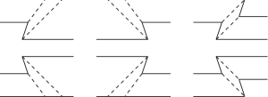
FIG. 3.: Time-ordered diagrams that contribute to ${\cal{R}}_{5}$. The diagrams in the first column have five particles in the first intermediate state. The diagrams in the second column have five particles in the last intermediate state, and the diagrams on the right have five-particle intermediate states for both the first and the third intermediate state.

This helps us to understand why ${\cal{R}}^{\rm LF}_{5}=0$. All contributing diagrams contain vacuum creation or annihilation vertices, which are forbidden by the spectrum condition.

There are twelve diagrams contributing to ${\cal{R}}_{6}$, and all contain vacuum creation or annihilation vertices. Therefore ${\cal{R}}^{\rm LF}_{6}$ vanishes.

We calculated ${\cal{R}}^{\rm IF}_{4^{+}}$ by subtracting the four diagrams only containing three particle intermediate states from the full sum. This sum can be obtained by doing the covariant calculation, or by adding all LF time-ordered boxes. Our results are given in Fig. 4. We also calculated ${\cal{R}}^{\rm IF}_{5^{+}}$.

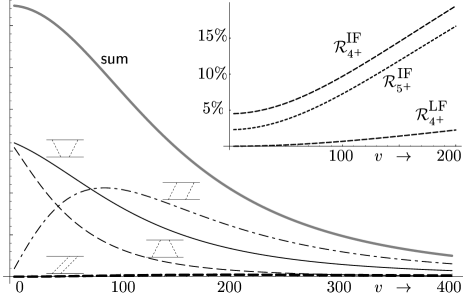
FIG. 4.: LF time-ordered boxes for a scattering angle of $\pi/2$ as a function of the incoming momentum $v$. We also give the ratios of boxes with at least four particles (${\cal{R}}^{\rm IF}_{4^{+}}$ and ${\cal{R}}^{\rm LF}_{4^{+}}$) or five particles (${\cal{R}}^{\rm IF}_{5^{+}}$, ${\cal{R}}^{\rm LF}_{5^{+}}=0$) in one of the intermediate states.

We conclude that on the LF contributions of higher Fock states are significantly smaller than in IFD. In the limit $v\rightarrow 0$ the ratio ${\cal{R}}^{\rm LF}_{4^{+}}$ goes to zero, because the phase space becomes empty. However, in IFD there is a finite contribution of ${\cal{R}}^{\rm IF}_{4^{+}}=4.5\%$ in this limit. Even if one includes five-particle intermediate states the LF is the winner by far.

Note that $m^{\prime}$, given by Eq. (55), varies as a function of $p^{2}$, and therefore also as a function of $v$, but is independent of $\alpha$. The deviation of $m^{\prime}$ from $m$ is small; less than 2.3% for $v<200$, and less than 9% for $v<400$. As the deviation of the mass $m^{\prime}$ from $m$ is only small, we are convinced that these results are indicative for calculations above threshold. However, we do not want to do these calculations, because then one needs to subtract the on-shell singularities of the equal-time ordered boxes.

VI Numerical results above threshold

As in Sec. V we look at the scattering of two particles over an angle of $\pi/2$. We focus on LFD, and therefore we simply write ${\cal{R}}_{4}={\cal{R}}^{\rm LF}_{4^{+}}$. We do no try to avoid on-shell singularities by taking different masses for the internal and external nucleons. Two nucleons of mass $m=940$ scatter via the exchange of scalar mesons of mass $\mu=140$. Again, the vertex is a scalar and no spin is included.

A Evaluation method

Contrary to the case considered in Sec. V, now it is not straightforward to evaluate the contributions of the LF time-ordered boxes, because the nonstretched boxes contain on-shell singularities, thoroughly analyzed in Sec. VIII. Here we briefly sketch how we deal numerically with the singularities. Using the analysis of Sec. VIII we identify the singularity $I_{\rm sing}$, and rewrite the nonstretched boxes as

$$\int{\rm d}^{3}k\;I=\int{\rm d}^{3}k(I-I_{\rm sing})+\int{\rm d}^{3}k\;I_{\rm sing}.$$ (56)

The integrand $I_{\rm sing}$ has a simple algebraic form, such that the integration in one dimension over the singularity can be done analytically, and the remaining integral is regular. This integral is then done numerically by mathematica. The integral over $(I-I_{\rm sing})$ was implemented in fortran. These two numbers are added to give the results presented is Secs. VI B and VI C.

B Results as a function of $\alpha$

We shall now vary the direction of $\vec{v^{\prime}}$, given by the azimuthal angle $\alpha$, however, not its length. Therefore the Mandelstam variables are independent of $\alpha$, and we expect the full amplitude to be invariant. We tested this numerically for a number of values of ${v}$. In the region $0\leq\alpha\leq\pi$ we used the formulas (40) until (43). In the region $\pi\leq\alpha\leq 2\pi$ the diagrams (41) and (43) vanish. However, then there are contributions from the diagrams in (44). The results are shown in Fig. 5. The results are normalized to the value of the covariant amplitude. The contributions from the different diagrams vary strongly with the angle $\alpha$. Since the imaginary parts are always positive, they are necessarily in the range $[0,1]$ when divided by the imaginary part of the covariant amplitude. The real parts can behave much more excentric, especially for higher values of the incoming c.m.s.-momentum $v$. An analysis of the $\alpha$-dependence is given in Sec. VIII. Clearly the LF time-ordered diagrams add up to the covariant amplitude, so we see that in all cases we obtain covariant (in particular rotationally invariant) results for both the real and the imaginary part.

C Numerical results as function of ${v}$

We look at scattering in the $x$-$z$-plane ($\alpha=\pi/2$), because in that case the contributions from the stretched boxes are maximized. The results are shown in Fig. 6.

We see that the stretched box, the diagram with two simultaneously exchanged mesons, is relatively small at low energies, but becomes rather important at higher energies. We depict the ratio of the stretched box to both the real part and to the total amplitude. Since the real part has a zero near $v=280$, the first ratio becomes infinite at that value of the incoming momentum.

[

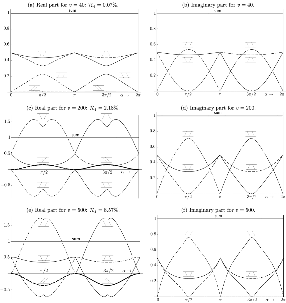
FIG. 5.: Amplitudes above threshold from $\alpha=0$ to $\alpha=2\pi$. ${\cal{R}}_{4}$ is the maximal fraction of the stretched box to the absolute value of the sum.

]

[

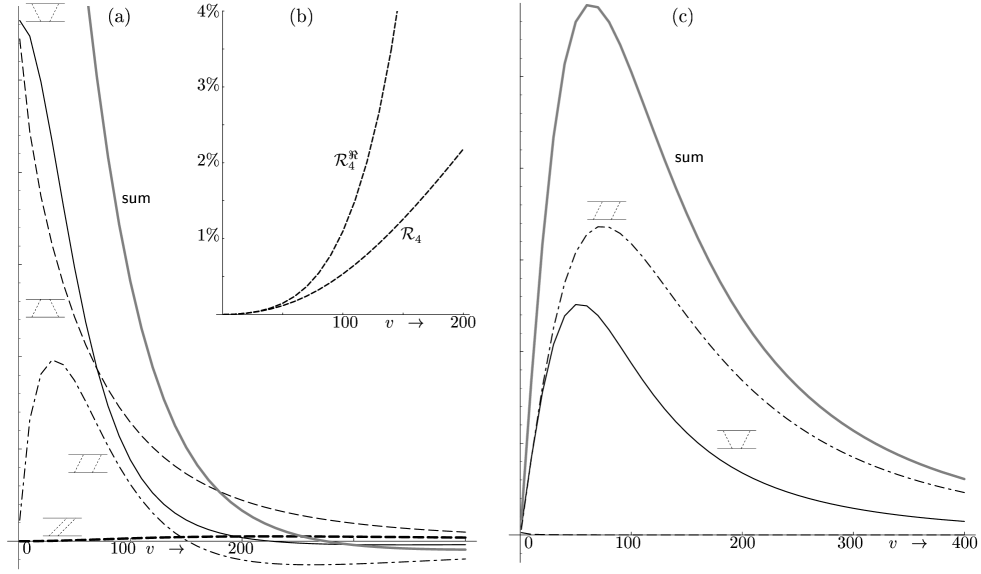
FIG. 6.: Real (a) and imaginary part (c) of the LF time-ordered boxes above threshold for $\alpha=\pi/2$ as a function of the momentum of the incoming particles $v$. The inset (b) shows the ratio of the stretched box to the real part of the amplitude (${\cal R}_{4}^{\Re}$) and to the absolute value (${\cal R}_{4}$).

]

VII Numerical results off energy-shell

In the previous section, we tested covariance of the LF formalism for amplitudes with on energy-shell external particles, by using the c.m. frame, where $P^{\perp}=p^{\prime\perp}+q^{\prime\perp}=0$ and $P^{z}=p^{\prime z}+q^{\prime z}=0$. However, on the LF the operator $P^{z}$ is dynamical, and the last equality does not hold anymore off energy-shell, as one can easily verify in the following way. Consider the case of a bound state with mass ${\cal M}<2m$. The bound state is off energy-shell, and therefore we have

$$P^{-}<p^{\prime-}+q^{\prime-}.$$ (57)

The plus and transverse momenta are kinematic, so

$$P^{+} = p^{\prime+}+q^{\prime+},$$ (58)

$$P^{\perp} = p^{\prime\perp}+q^{\prime\perp}.$$ (59)

Adding Eqs. (57) and (58) gives

$$P^{z}<p^{\prime z}+q^{\prime z}.$$ (60)

If $P^{z}=0$, then Eq. (60) implies that $p^{\prime z}+q^{\prime z}>0$. Therefore the two outgoing particles cannot have exactly opposite momenta as in Eqs. (47) and (48). In terms of the explicitly covariant LFD, introduced in Sec. VIII, this reflects the fact that the off energy-shell relation between $p^{\prime}+q^{\prime}$ and $P$ contains extra four-momentum like in Eq. (133). What was the reason that we chose opposite momenta in the previous sections in the first place? Our reason was that we wanted to have a manifest symmetry of the amplitude, because it is obvious that the Mandelstam variables $s$, $t$ and $u$ remain the same under the rotations we investigated. We investigate how the off-shell amplitude breaks covariance by using momenta for the outgoing particles, such that the Mandelstam variables remain constant, at the same time satisfying the conditions (57)-(60).

As in the previous sections, we shall fix the direction of the incoming particles, as in Eqs. (45) and  (46), and vary the direction of the outgoing particles. Therefore, by construction, $s$ is invariant. In order to guarantee the invariance of the other Mandelstam variables $t$ and $u$ we must take $p\!\cdot\!q^{\prime}$ and $p\!\cdot\!p^{\prime}$ constant, even off energy-shell. These inner products are:

$$p\!\cdot\!q^{\prime}=p^{+}q^{\prime-}+q^{\prime+}p^{-}-p^{\perp}\!\cdot\!q^{\prime\perp}\hskip 85.35826pt$$ (61)

$$=x_{p}P^{+}\frac{{q^{\prime\perp}}^{2}\!\!+m^{2}}{2(1\!-\!x_{p^{\prime}})P^{+}}+(1\!-\!x_{p^{\prime}})P^{+}\frac{{p^{\perp}}^{2}\!\!+m^{2}}{2x_{p}P^{+}}-p^{\perp}\!\!\cdot\!q^{\prime\perp},$$ (62)

$$p\!\cdot\!p^{\prime}=p^{+}p^{\prime-}+p^{\prime+}p^{-}-p^{\perp}\!\!\cdot\!p^{\prime\perp}\hskip 85.35826pt$$ (63)

$$=x_{p}P^{+}\frac{{q^{\prime\perp}}^{2}+m^{2}}{2x_{p^{\prime}}P^{+}}+x_{p^{\prime}}P^{+}\frac{{p^{\perp}}^{2}+m^{2}}{2x_{p}P^{+}}-p^{\perp}\!\!\cdot\!p^{\prime\perp}.$$ (64)

We have introduced the fractions

$$x_{p}=p^{+}/P^{+},\quad x_{p^{\prime}}=p^{\prime+}/P^{+}.$$ (65)

Since the perpendicular momenta are conserved we have in the c.m. system $p^{\prime\perp}=-q^{\prime\perp},$ so the inner products of the perpendicular momenta can be written as

$$p^{\perp}\!\!\cdot\!p^{\prime\perp}=\phantom{-}|p^{\perp}||p^{\prime\perp}|\cos\theta,$$ (66)

$$p^{\perp}\!\!\cdot\!q^{\prime\perp}=-|p^{\perp}||p^{\prime\perp}|\cos\theta,$$ (67)

where $\theta$ is the scattering angle. We can now solve Eqs. (61-66) for $x_{p^{\prime}}$, $|p^{\prime\perp}|$ and $\theta$. There are many curves satisfying these conditions. For uniqueness we demand that the curve goes through the point in which $x_{p^{\prime}}=x_{p}=1/2$, $|p^{\prime\perp}|=|p^{\perp}|$ and $\theta=\pi/2$. We find that the curve is then parametrized by

$$\theta = \pi/2,$$ (68)

$$\frac{{p^{\prime\perp}}^{2}+m^{2}}{x_{p^{\prime}}(1\!-\!x_{p^{\prime}})} = 4({p^{\perp}}^{2}+m^{2}).$$ (69)

From $x_{p^{\prime}}$ and $p^{\prime\perp}$ we determine $p^{\prime+}$ and $p^{\prime-}$ , and finally also $p^{\prime z}$. Because the particles come in along the $x$-axis, the above relations define an ellipse in the $y$-$z$-plane. In the case of IFD these ellipses would reduce to circles with center of the origin and radius $v$.

FIG. 7.: Possible momenta $p^{\prime}$ and $q^{\prime}$ of the outgoing particles (fat line) in the scattering plane (horizontal: $p^{\prime y}$ and $q^{\prime y}$, vertical: $p^{\prime z}$ and $q^{\prime z}$) for two cases: (a) $v=40$ and (b) $v=200$. The momentum $p^{\prime}+q^{\prime}$ is indicated by the dot. As a reference we have drawn the locus for on energy-shell external particles (thin line): a circle centered at the origin.

In Fig. 7 we have indicated the $y$ and $z$-components of the momenta of the external particles for the two cases we investigate. We see that Eqs. (59) and (60) hold. The off energy-shell momenta form an ellipse. The deviation from a circle with radius $v$ is hardly visible.

In Fig. 8 we show the contributions of the different boxes and their sum as we vary the angle $\alpha$. The calculations are the same as in the previous section, using the formulas (40)-(44), except that the momenta of the outgoing particles have changed such that (68) and (69) are satisfied. As there does not exist a covariant amplitude in the off energy-shell case, we normalized the curves shown by dividing the amplitudes by their sum at $\alpha=\pi/4$.

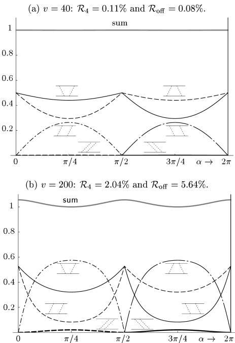
FIG. 8.: The LF time-ordered boxes as a function of $\alpha$.

In Fig. 8 we see the consequences of the off energy-shell initial and final states. Condition (28) is violated, therefore Eq. (30) does not hold and a breaking of covariance can be expected. We see that the contributions of the higher Fock states ${\cal R}_{4}$ are smaller than the effect of the off-shellness ${\cal R}_{\rm off}$. This is confirmed in Fig. 9, in which $\alpha$ is fixed and the incoming c.m.s-momentum $v$ is varied.

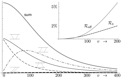
FIG. 9.: The LF time-ordered boxes as a function of $v$ for $\alpha=\pi/2$. The inset shows the maximum contributions of the stretched box, and the maximal breaking of covariance.

From Fig. 8 we infer that the full amplitude is maximal at $\alpha=0$ and $\alpha=\pi$. The minimum is reached at $\alpha=\pi/2$ and $\alpha=3\pi/2$. Therefore the maximal breaking of covariance of the amplitude can be calculated by taking the difference of the total sum at the angles $\alpha=0$ and $\alpha=\pi/2$. We see that at typical values for incoming momentum ($v\leq 50$) ${\cal R}_{\rm off}$ is small, even smaller than ${\cal R}_{4}$. However, at higher momenta it dominates over the stretched box. In this region we see that the stretched box contributions remain small.

A detailed explanation of the results for off energy-shell amplitudes is given in Sec. IX.

VIII Analysis of the on energy-shell results

The angle dependence of the LF time-ordered amplitudes found numerically, can be understood analytically. The variation of the LF amplitudes with the angle $\alpha$ means that they have singularities in this variable, either at finite values of $\alpha$ or at infinity. They should disappear when they are summed to give the covariant amplitude. These singularities can be most conveniently analyzed in the explicitly covariant version of LFD (see for a review [3]). In this version the orientation of the light-front is given by the invariant equation $\omega\makebox[2.27626pt]{$\cdot$}x=0$. The amplitudes are calculated by the rules of the graph technique explained in Ref. [3]. After a transformation of variables, these amplitudes coincide with those given by ordinary LFD. However, they are parametrized in a different way. The dependence of the amplitudes on the angle $\alpha$ means, in the covariant version, that they depend on the four-vector $\omega$ determining the orientation of the LF plane: $M=M(p,q,p^{\prime},q^{\prime},\omega)$. Hence, besides the usual Mandelstam variables $s$ (50) and $t$ (51) the amplitude $M$ depends on the scalar products of $\omega$ with the four-momenta. Since $\omega$ determines the direction only (the theory is invariant relative to the substitution $\omega\rightarrow a\omega$), an amplitude should depend on the ratios of the scalar products of the four-momenta with $\omega$. Hence [15]:

$$M=M(s,t,x_{p},x_{p^{\prime}}),$$ (70)

where

$$x_{p}=\frac{\omega\makebox[2.27626pt]{$\cdot$}p}{\omega\makebox[2.27626pt]{$\cdot$}(p+q)},\quad x_{p^{\prime}}=\frac{\omega\makebox[2.27626pt]{$\cdot$}p^{\prime}}{\omega\makebox[2.27626pt]{$\cdot$}(p+q)}.$$ (71)

The formulas (71) coincide with the definitions (65) if we use the $z$-axis as the quantization axis. The $\omega$-dependence is reduced to two scalar variables $x_{p}$ and $x_{p^{\prime}}$, since the direction of $\vec{\omega}$ is determined by two angles. Hence, this amplitude should have singularities in the variables $x_{p}$ and $x_{p^{\prime}}$. Their positions will be found below. The amplitude corresponding to the sum of all time-ordered diagrams should not depend on $x_{p}$ and $x_{p^{\prime}}$.

Let us find the physical domain of the variables $x_{p}$ and $x_{p^{\prime}}$, corresponding to all possible directions of $\vec{\omega}$ for fixed $s,t$. In the c.m. system the variables Eq. (71) are represented as:

$$x_{p}=\frac{1}{2}-\frac{v}{\sqrt{s}}\hat{\omega}\!\cdot\!\hat{p},\quad x_{p^{\prime}}=\frac{1}{2}-\frac{v}{\sqrt{s}}\hat{\omega}\!\cdot\!\hat{p}^{\prime},$$ (72)

where, e.g., $\hat{\omega}\!\cdot\!\hat{p}$ is the scalar product of the unit vectors $\hat{\omega}=\vec{\omega}/|\vec{\omega}|$ and $\hat{p}=\vec{p}/|\vec{p}|$ in three-dimensional Euclidian space, and $v=\sqrt{s/4-m^{2}}$ is the momentum of the particle in the c.m. system. The Eqs. (72) determine an ellipse in the $x_{p}$-$x_{p^{\prime}}$-plane. Its boundary is obtained when $\vec{\omega}$ is in the scattering plane, that is $\hat{n}\!\cdot\!\hat{p}=\cos\gamma$ or $\hat{n}\!\cdot\!\hat{p}=\cos(\gamma-\theta)$, where $\gamma$ is the angle between $\vec{p}$ and $\vec{\omega}$ in coplanar kinematics and $\theta$ is the scattering angle in the c.m.s. The case when $\vec{\omega}$ is out of the scattering plane corresponds to the interior of the ellipse. For a scattering angle $\theta=\pi/2$ the ellipse turns into a circle, shown in Fig. 10.

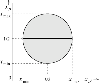
FIG. 10.: Physical region in the $x_{p}$-$x_{p^{\prime}}$-plane.

For the kinematics shown in Fig. 2 and Eqs. (45)-(48), i.e., when $\vec{\omega}\perp\vec{p}$, it follows from Eq. (72) that the value $x_{p}$ is fixed: $x_{p}=\frac{1}{2},$ whereas for a given $\alpha$ we obtain:

$$x_{p^{\prime}}=\frac{1}{2}-\frac{v}{2v_{0}}\sin\alpha,$$ (73)

with $v_{0}=\sqrt{m^{2}+v^{2}}$, varies along a straight line when $\hat{\omega}$ is rotated in the $y$-$z$-plane. The bounds of the physical region of $x_{p^{\prime}}$ are:

$$x_{\rm min}=\frac{1}{2}-\frac{v}{2v_{0}},\quad x_{\rm max}=\frac{1}{2}+\frac{v}{2v_{0}}.$$ (74)

When $0\leq\alpha\leq\pi/2$, $x_{p^{\prime}}$ moves from 1/2 to $x_{\rm min}$. When $\pi/2\leq\alpha\leq\pi$, $x_{p^{\prime}}$ moves in the opposite direction in the same interval. This explains why all the curves in Figs. 5 and 8 in the interval $0\leq\alpha\leq\pi$ are symmetric relative to $\alpha=\pi/2$.

When $\pi\leq\alpha\leq 3\pi/2$, $x_{p^{\prime}}$ moves from 1/2 to $x_{\rm max}$ and, finally, when $3\pi/2\leq\alpha\leq 2\pi$, it goes back in the same interval. As in the previous paragraph, this explains why all the curves in Figs. 5 and  8 in the interval $\pi\leq\alpha\leq 2\pi$ are symmetric relative to $\alpha=3\pi/2$. When $\alpha=\pi/2$ and $3\pi/2$, the values of $x_{p^{\prime}}$ are on the boundary of the physical region.

Note also that the amplitudes for the trapezium (dashed and solid curves in Figs. 5 and 8) are evidently obtained by the replacement $p\leftrightarrow q,\quad p^{\prime}\leftrightarrow q^{\prime}$, which, according to the definition in Eq. (71), corresponds to $x_{p^{\prime}}\rightarrow 1-x_{p^{\prime}}$. This is the same as the replacement $\alpha\rightarrow 2\pi-\alpha$ in Eq. (73). Therefore the curves for the other trapezium, when $\alpha$ goes from $2\pi$ to 0, repeat the curves for the trapezium, when $\alpha$ increases from 0 to $2\pi$. The same is true for the other diagrams (diamonds and stretched boxes).

A Trapezium

The method of finding the singularities of the LF diagrams was developed in [15]. Here we restrict ourselves to the example of the diagram (40). Its counterpart in the explicitly covariant LFD is shown in Fig. 11.

FIG. 11.: The trapezium in explicitly covariant LFD.

The dotted lines in this figure are associated with fictitous particles (spurions), with four-momenta proportional to $\omega$. The four-momenta of the particles (the spurions not included) are not conserved in the vertices. Conservation is restored by taking into account the spurion four-momentum. In the ordinary LF approach this corresponds to nonconservation of the minus-components of the particles. The spurions make up for the difference.

According to the rules of the graph techniques [3], one should associate with a particle line with four-momentum $p$ and mass $m$ the factor $\theta(\omega\makebox[2.27626pt]{$\cdot$}p)\delta(p^{2}-m^{2})$ and associate with the spurion line with four-momentum $\omega\tau_{i}$ the factor $1/(\tau_{i}-i\epsilon)$. Then one integrates, with measure d${}^{4}k_{i}/(2\pi)^{3}$, over all the four-momenta $k_{i}$ not restricted by the conservation laws in the vertices, and over all ${\rm d}\tau_{i}$. The expression for the amplitude of Fig. 11 is:

$$= \int\theta(\omega\makebox[2.27626pt]{$\cdot$}k)\delta(k^{2}-m^{2})$$ (79)

$$\times\theta(\omega\makebox[2.27626pt]{$\cdot$}(p^{\prime}-k))\ \delta((p^{\prime}-k+\omega\tau_{1})^{2}-\mu^{2})$$

$$\times\theta(\omega\makebox[2.27626pt]{$\cdot$}(p+q-k))\ \delta((p+q-k+\omega\tau_{2})^{2}-m^{2})$$

$$\times\theta(\omega\makebox[2.27626pt]{$\cdot$}(p-k))\ \delta((p-k+\omega\tau_{3})^{2}-\mu^{2})$$

$$\times\frac{{\rm d}\tau_{1}}{(\tau_{1}-i\epsilon)}\frac{{\rm d}\tau_{2}}{(\tau_{2}-i\epsilon)}\frac{{\rm d}\tau_{3}}{(\tau_{3}-i\epsilon)}\frac{{\rm d}^{4}k}{(2\pi)^{3}}\ .$$

Like in Eq. (26), we omit the coupling constant. Performing the integrals over $\tau_{i}$ and ${\rm d}k_{0}$ in Eq. (79) by means of the $\delta$-functions, we get:

$$\raisebox{-7.11317pt}{\epsfbox{bokns1.eps}}=\int\frac{\theta(\omega\makebox[2.27626pt]{$\cdot$}(p^{\prime}-k))}{\mu^{2}-(p^{\prime}-k)^{2}}\ \frac{\theta(\omega\makebox[2.27626pt]{$\cdot$}(p+q-k))}{m^{2}-(p+q-k)^{2}}$$ (80)

$$\times\;\frac{\theta(\omega\makebox[2.27626pt]{$\cdot$}(p-k))}{\mu^{2}-(p-k)^{2}}\ \theta(\omega\makebox[2.27626pt]{$\cdot$}k)\frac{{\rm d}^{3}k}{2\varepsilon_{k}(2\pi)^{3}}.$$ (81)

By transformations of variables (see for the details appendix B of [3]) the expression Eq. (81) can be transformed such that it exactly coincides with Eq. (40).

For Feynman amplitudes the method to find their singularities was developed by Landau in [16]. A method very similar to that one can be applied to time-ordered amplitudes. If we would omit for a moment the $\theta$-functions in Eq. (81) and would not take into account that $k^{2}=m^{2}$, for finding the singularities we should construct the function $\varphi_{1}=\alpha_{1}(\mu^{2}-(p^{\prime}-k)^{2})+\alpha_{2}(m^{2}-(p+q-k)^{2})+\alpha_{3}(m^{2}-(p-k)^{2})$ formed from the denominator of (80). The singularities of the trapezium are found by putting to zero the derivatives of $\varphi_{1}$ with respect to $\alpha_{1-3}$ and with respect to $k$. However, the trapezium may have singularities corresponding to a coincidence of the singularities of its integrand with the boundary of the integration domain caused by the presence of the $\theta$-functions. So, we must find a conditional extremum. The restrictions can be taken into account using Lagrange multipliers [15]. Hence, we should consider the function:

$$\varphi=\alpha_{1}(\mu^{2}-(p^{\prime}-k)^{2})+\alpha_{2}(m^{2}-(p+q-k)^{2})$$ (82)

$$+\alpha_{3}(\mu^{2}-(p-k)^{2})+\alpha_{4}(k^{2}-m^{2})+\gamma_{1}\omega\makebox[2.27626pt]{$\cdot$}(k-p^{\prime}),$$ (83)

where $\alpha_{4}$ and $\gamma_{1}$ are the Lagrange multipliers. One should also consider the functions obtained from $\varphi$ at $\alpha_{1}=0$, then at $\alpha_{2}=0$, then $\alpha_{3}=0$, then at $\alpha_{1}=\alpha_{2}=0$, etc. One should not consider the function obtained from (83) by $\alpha_{4}=0$, since the integral (81) contains the three-dimensional integration volume ${\rm d}^{3}k$, and the condition $k^{2}=m^{2}$ cannot be deleted. Therefore there is no need to introduce the term $\gamma_{2}\omega\makebox[2.27626pt]{$\cdot$}k$, since the $k^{2}=m^{2}$ condition prevents this term from being zero and, hence, does not impose any restrictions. The case $\gamma_{1}=0$ reproduces the singularities of the Feynman graph. Therefore below we shall consider the case $\gamma_{1}\neq 0$ resulting in the singularities in the variables $x_{p},x_{p^{\prime}}$. We suppose that $\omega\makebox[2.27626pt]{$\cdot$}p\geq\omega\makebox[2.27626pt]{$\cdot$}p^{\prime}.$ This corresponds to the condition $p^{+}\geq p^{\prime+}$ of Sec. III. In the kinematics shown in Fig. 2 this means that $x_{p^{\prime}}\leq 1/2$ and $0\leq\alpha\leq\pi$. In this case, the second and the third $\theta$-functions in Eq. (81) do not give any restrictions and can be omitted. Therefore we omit also the term $\gamma_{3}\omega\makebox[2.27626pt]{$\cdot$}(p-k)+\gamma_{4}\omega\makebox[2.27626pt]{$\cdot$}(p+q-k)$.

The derivatives of $\varphi$ with respect to $k$, the $\alpha$’s and $\gamma_{1}$ give:

$$\partial\varphi/\partial k=\alpha_{1}2(p^{\prime}-k)+\alpha_{2}2(p+q-k)$$ (84)

$$+\alpha_{3}2(p-k)+\alpha_{4}2k+\gamma_{1}\omega=0,$$ (85)

with

$$(p^{\prime}-k)^{2} = \mu^{2},\quad(p+q-k)^{2}=m^{2},$$ (86)

$$(p-k)^{2} = \mu^{2},\quad k^{2}=m^{2},\quad\omega\makebox[2.27626pt]{$\cdot$}k=\omega\makebox[2.27626pt]{$\cdot$}p^{\prime}.$$ (87)

[We multiply Eq. (85) in turn by $(p^{\prime}-k)$, $(p+q-k)$, et cetera, and get:

$$\begin{array}[]{ll}(\ref{eq19})\times p^{\prime}-k:&\alpha_{1}2\mu^{2}+\alpha_{2}\mu^{2}+\alpha_{3}(2\mu^{2}-t)-\alpha_{4}\mu^{2}=0,\\ (\ref{eq19})\times p+q-k:&\alpha_{1}\mu^{2}+\alpha_{2}2m^{2}+\alpha_{3}\mu^{2}+\alpha_{4}(s-2m^{2})+\gamma_{1}(1-x_{p^{\prime}})=0,\\ (\ref{eq19})\times p-k:&\alpha_{1}(2\mu^{2}-t)+\alpha_{2}\mu^{2}+\alpha_{3}2\mu^{2}-\alpha_{4}\mu^{2}+\gamma_{1}(x_{p}-x_{p^{\prime}})=0,\\ (\ref{eq19})\times k:&-\alpha_{1}\mu^{2}+\alpha_{2}(s-2m^{2})-\alpha_{3}\mu^{2}+2\alpha_{4}m^{2}+\gamma_{1}x_{p^{\prime}}=0,\\ (\ref{eq19})\times\omega:&\alpha_{2}(1-x_{p^{\prime}})+\alpha_{3}(x_{p}-x_{p^{\prime}})+\alpha_{4}x_{p^{\prime}}=0.\end{array}$$ (88)

These equations have a nontrivial solution iff:

$$\left|\begin{array}[]{lllll}2\mu^{2}&\mu^{2}&(2\mu^{2}-t)&-\mu^{2}&0\\ \mu^{2}&2m^{2}&\mu^{2}&(s-2m^{2})&(1-x_{p^{\prime}})\\ (2\mu^{2}-t)&\mu^{2}&2\mu^{2}&-\mu^{2}&(x_{p}-x_{p^{\prime}})\\ -\mu^{2}&(s-2m^{2})&-\mu^{2}&2m^{2}&x_{p^{\prime}}\\ 0&(1-x_{p^{\prime}})&(x_{p}-x_{p^{\prime}})&x_{p^{\prime}}&0\end{array}\right|=0.$$ (89)

] Eq. (89) is quadratic in $x_{p^{\prime}}$. Its solution is simple but lengthy. We show it for the particular case of the kinematics of Fig. 2 supposing that the particles in the c.m. system have momenta $v$. In this case $s$ and $t$ are given by Eqs. (50) and (51). The solution of Eq. (89) is:

$$x_{p^{\prime}}^{0}=\frac{1}{2}\pm\frac{v}{2v_{0}}\frac{\sqrt{2\mu^{4}+8\mu^{2}v^{2}+4v^{4}}}{\sqrt{\mu^{4}+8\mu^{2}v^{2}+4v^{4}}}.$$ (90)

The position of singularity in the variable $x_{p^{\prime}}$ is denoted by $x^{0}_{p^{\prime}}$. According to [16] the behavior in the vicinity of $x_{p^{\prime}}^{0}$ should be either logarithmic, proportional to $|x_{p^{\prime}}-x_{p^{\prime}}^{0}|^{\beta}$, or proportional to $|x_{p^{\prime}}-x_{p^{\prime}}^{0}|^{\beta}\log(x_{p^{\prime}}-x_{p^{\prime}}^{0})$, where $\beta$ is a noninteger number.

When $\mu\ll v$ we find from Eq. (90):

$$x_{p^{\prime}}=\frac{1}{2}\pm\frac{v}{2v_{0}}(1+\frac{\mu^{4}}{8v^{4}}).$$ (91)

Comparing with Eq. (74), we see that at small $\mu$ or at large $v$ the singularities come closer to the physical region of $x_{p^{\prime}}$. We will see below that this will be a property of all the singularities depending on $\mu$ and $v$. This explains the numerical results, showing that with an increase of $v$ the graphs of the amplitudes versus $\alpha$ become more sharply peaked.

Now consider the case when one of the $\alpha$’s is zero. Let $\alpha_{1}=0$. Then Eq. (83) is reduced to:

$$\varphi=\alpha_{2}(m^{2}-(p+q-k)^{2})+\alpha_{3}(\mu^{2}-(p-k)^{2})$$ (92)

$$+\alpha_{4}(k^{2}-m^{2})+\gamma_{1}\omega\makebox[2.27626pt]{$\cdot$}(k-p^{\prime}).$$ (93)

Similarly to the previous case we get an equation, which can be obtained from Eq. (89) by deleting the first row and column:

$$\left|\begin{array}[]{lllll}2m^{2}&\mu^{2}&(s-2m^{2})&(1-x_{p^{\prime}})\\ \mu^{2}&2\mu^{2}&-\mu^{2}&(x_{p}-x_{p^{\prime}})\\ (s-2m^{2})&-\mu^{2}&2m^{2}&x_{p^{\prime}}\\ (1-x_{p^{\prime}})&(x_{p}-x_{p^{\prime}})&x_{p^{\prime}}&0\end{array}\right|=0.$$ (94)

Under the given kinematical conditions its solution with respect to $x_{p^{\prime}}$ is

$$x_{p^{\prime}}^{0}=\frac{1}{2}\pm\frac{\mu}{4v}\sqrt{\frac{\mu^{2}+4v^{2}}{m^{2}+v^{2}}}.$$ (95)

In the limit $\mu\rightarrow 0$ or $v\rightarrow\infty$ these singularities are again approaching the physical region.

Let $\alpha_{2}=0$. The equation is obtained from Eq. (89) by deleting the second row and column:

$$\left|\begin{array}[]{lllll}2\mu^{2}&(2\mu^{2}-t)&-\mu^{2}&0\\ (2\mu^{2}-t)&2\mu^{2}&-\mu^{2}&(x_{p}-x_{p^{\prime}})\\ -\mu^{2}&-\mu^{2}&2m^{2}&x_{p^{\prime}}\\ 0&(x_{p}-x_{p^{\prime}})&x_{p^{\prime}}&0\end{array}\right|=0.$$ (96)

Its solution reads:

$$x_{p^{\prime}}^{0}=\frac{x_{p}\mu(4m^{2}\mu-\mu^{3}-\mu t\pm 2\sqrt{t}\sqrt{tm^{2}+\mu^{4}-4m^{2}\mu^{2}})}{4m^{2}\mu^{2}-(t-\mu^{2})^{2}}.$$ (97)

In the limit $v\rightarrow\infty$ it is simplified:

$$x_{p^{\prime}}^{0}=-\frac{\mu^{2}}{4v^{2}}\pm\frac{\mu m}{2v^{2}}.$$ (98)

Let $\alpha_{3}=0$. The equation is obtained from Eq. (89) by deleting the third row and column:

$$\left|\begin{array}[]{lllll}2\mu^{2}&\mu^{2}&-\mu^{2}&0\\ \mu^{2}&2m^{2}&(s-2m^{2})&(1-x_{p^{\prime}})\\ -\mu^{2}&(s-2m^{2})&2m^{2}&x_{p^{\prime}}\\ 0&(1-x_{p^{\prime}})&x_{p^{\prime}}&0\end{array}\right|=0.$$ (99)

The determinant in Eq. (99) can be evaluated:

$$4sx_{p^{\prime}}^{2}-4sx_{p^{\prime}}+4m^{2}-\mu^{2}=0.$$ (100)

The solutions of Eq. (100) are:

$$x_{p^{\prime}}^{0}=\frac{1}{2}\pm\frac{\sqrt{v^{2}+\mu^{2}/4}}{2v_{0}}.$$ (101)

For $\mu\rightarrow 0$ they also approach the boundary of the physical region of $x_{p^{\prime}}$.

Now consider the cases when a few coefficients are zero. Let $\alpha_{1}=\alpha_{3}=0$. The equation can be obtained from Eq. (89) by deleting the first and third rows and columns:

$$\left|\begin{array}[]{lllll}2m^{2}&(s-2m^{2})&(1-x_{p^{\prime}})\\ (s-2m^{2})&2m^{2}&x_{p^{\prime}}\\ (1-x_{p^{\prime}})&x_{p^{\prime}}&0\end{array}\right|=0.$$ (102)

This equation reduces to:

$$x_{p^{\prime}}^{2}-x_{p^{\prime}}s+m^{2}=0.$$ (103)

Its solutions are:

$$x_{p^{\prime}}^{0}=\frac{1}{2}+\frac{v}{2v_{0}}=x_{{\rm max}},\;\;x_{p^{\prime}}^{0}=\frac{1}{2}-\frac{v}{2v_{0}}=x_{{\rm min}}.$$ (104)

Since we consider the interval $0\leq\alpha\leq\pi$ corresponding to $x_{\rm min}\leq x_{p^{\prime}}\leq 1/2$, the singularity at $x_{p^{\prime}}^{0}=x_{\rm max}$ is beyond the physical region, whereas the singularity at $x_{p^{\prime}}^{0}=x_{\rm min}$ is just on the boundary of the physical region. The amplitude in this point gets an imaginary part:

$${\rm Im}\;\raisebox{-7.11317pt}{\epsfbox{bokns1.eps}}\;\neq 0{\;\;\rm at\;\;}x_{p^{\prime}}>x_{\rm min},$$ (105)

$${\rm Im}\;\raisebox{-7.11317pt}{\epsfbox{bokns1.eps}}\;=0{\;\;\rm at\;\;}x_{p^{\prime}}=x_{\rm min}.$$ (106)

Eq. (106) corresponds to $\alpha=\pi/2$. This explains, why all the dashed curves of the imaginary parts in Fig. 5 go through zero at the point $\alpha=\pi/2$.

Now put $\alpha_{1}=\alpha_{2}=0$. The corresponding equation is obtained from Eq. (89) by deleting the first and second rows and columns:

$$\left|\begin{array}[]{lllll}2\mu^{2}&-\mu^{2}&(x_{p}-x_{p^{\prime}})\\ -\mu^{2}&2m^{2}&x_{p^{\prime}}\\ (x_{p}-x_{p^{\prime}})&x_{p^{\prime}}&0\end{array}\right|=0.$$ (107)

Eq. (107) reads:

$$x_{p^{\prime}}^{2}m^{2}-x_{p^{\prime}}x_{p}(2m^{2}-\mu^{2})+x_{p}^{2}m^{2}=0.$$ (108)

Its solution is:

$$x_{p^{\prime}}^{0}=\frac{x_{p}}{2m^{2}}\left(2m^{2}-\mu^{2}\pm i\mu\sqrt{4m^{2}-\mu^{2}}\right).$$ (109)

These two singularities are fixed points in the complex plane. At $x_{p}=1/2$ and $\mu\ll m$ they are approaching the point $x_{p^{\prime}}=1/2$ in the physical region, i.e., $\alpha=0$ and $\alpha=\pi$.

The case $\alpha_{2}=\alpha_{3}=0$ leads to the equation obtained from Eq. (89) by deleting the second and third rows and columns:

$$\left|\begin{array}[]{lllll}2\mu^{2}&-\mu^{2}&0\\ -\mu^{2}&2m^{2}&x_{p^{\prime}}\\ 0&x_{p^{\prime}}&0\end{array}\right|=0.$$ (110)

It gives $x_{p^{\prime}}^{0}=0$. This is a fixed singularity in the nonphysical region.

Above we have considered the region $\omega\makebox[2.27626pt]{$\cdot$}p\geq\omega\makebox[2.27626pt]{$\cdot$}p^{\prime}$. In the region $\omega\makebox[2.27626pt]{$\cdot$}p\leq\omega\makebox[2.27626pt]{$\cdot$}p^{\prime}$ the integration domain is restricted by the step function $\theta(\omega\makebox[2.27626pt]{$\cdot$}(p-k))$ instead of $\theta(\omega\makebox[2.27626pt]{$\cdot$}(p^{\prime}-k))$ in Eq. (81). The integrals defining these amplitudes define different analytic functions depending on the region considered. In the point $x_{p^{\prime}}=1/2$, i.e. at $\alpha=0$ and $\alpha=\pi$, the values of the functions coincide, but their analytic behavior is different.

This can indeed be seen in Fig. 5. The slopes at $\alpha=0$ and $\alpha=\pi$ are different.

B Diamond

The diamond corresponding to Eq. (41) is shown in Fig. 12.

FIG. 12.: The diamond in explicitly covariant LFD.

The analytical expression is:

$$= \int\theta(\omega\makebox[2.27626pt]{$\cdot$}k)\delta(k^{2}-m^{2})$$ (115)

$$\times\theta(\omega\makebox[2.27626pt]{$\cdot$}(k-p^{\prime}))\delta((k-p^{\prime}+\omega\tau_{1}-\omega\tau_{2})^{2}-\mu^{2})$$

$$\times\theta(\omega\makebox[2.27626pt]{$\cdot$}(p+q-k))\delta((p+q-k+\omega\tau_{2})^{2}-m^{2})$$

$$\times\theta(\omega\makebox[2.27626pt]{$\cdot$}(p-k))\delta((p-k+\omega\tau_{3})^{2}-\mu^{2})$$

$$\times\frac{{\rm d}\tau_{1}{\rm d}\tau_{2}{\rm d}\tau_{3}}{(\tau_{1}-i\epsilon)(\tau_{2}-i\epsilon)(\tau_{3}-i\epsilon)}\frac{{\rm d}^{4}k}{(2\pi)^{3}}.$$

Performing the integrations in Eq. (115) over $\tau_{i}$, we get:

$$\raisebox{-7.11317pt}{\epsfbox{bokns2.eps}}=$$ (117)

$$\int\frac{\theta(\omega\makebox[2.27626pt]{$\cdot$}(k-p^{\prime}))}{\mu^{2}-(k-p^{\prime})^{2}+\frac{\displaystyle{\omega\makebox[2.27626pt]{$\cdot$}(k-p^{\prime})}}{\displaystyle{\omega\makebox[2.27626pt]{$\cdot$}(p+q-k)}}[m^{2}-(p+q-k)^{2}]}$$ (118)

$$\times\frac{\theta(\omega\makebox[2.27626pt]{$\cdot$}(p+q-k))}{m^{2}-(p+q-k)^{2}}\frac{\theta(\omega\makebox[2.27626pt]{$\cdot$}(p-k))}{\mu^{2}-(p-k)^{2}}\ \theta(\omega\makebox[2.27626pt]{$\cdot$}k)\frac{{\rm d}^{3}k}{2\varepsilon_{k}(2\pi)^{3}}.$$ (119)

We still suppose that $\omega\makebox[2.27626pt]{$\cdot$}p>\omega\makebox[2.27626pt]{$\cdot$}p^{\prime}$. However, now, in contrast to the trapezium, $\omega\makebox[2.27626pt]{$\cdot$}p^{\prime}\leq\omega\makebox[2.27626pt]{$\cdot$}k\leq\omega\makebox[2.27626pt]{$\cdot$}p,$ and both restrictions have to be taken into account.

In order to find the singularities, one should consider the extremum of the function: [

$$\varphi = \alpha_{1}\left\{\mu^{2}-(k-p^{\prime})^{2}+\frac{\displaystyle{\omega\makebox[2.27626pt]{$\cdot$}(k-p^{\prime})}}{\displaystyle{\omega\makebox[2.27626pt]{$\cdot$}(p+q-k)}}(m^{2}-(p+q-k)^{2})\right\}$$ (122)

$$+\alpha_{2}\left\{m^{2}-(p+q-k)^{2}\right\}+\alpha_{3}\left\{\mu^{2}-(p-k)^{2}\right\}+\alpha_{4}(k^{2}-m^{2})$$

$$+\gamma_{1}\omega\makebox[2.27626pt]{$\cdot$}(k-p^{\prime})+\gamma_{2}\omega\makebox[2.27626pt]{$\cdot$}(k-p).$$

At $\omega\makebox[2.27626pt]{$\cdot$}p^{\prime}=\omega\makebox[2.27626pt]{$\cdot$}p$, i.e. at $\alpha=0$ and $\alpha=\pi$ the integration domain vanishes and the diamond becomes zero, as shown in Fig. 5. It remains zero in the interval $\pi\leq\alpha\leq 2\pi$.

C Stretched box

The stretched box, corresponding to Eq. (43) is shown in Fig. 13.

FIG. 13.: The stretched box in explicitly covariant LFD.

The analytical expression is:

$$= \int\theta(\omega\makebox[2.27626pt]{$\cdot$}k)\delta(k^{2}-m^{2})$$ (127)

$$\times\theta(\omega\makebox[2.27626pt]{$\cdot$}(k-p^{\prime}))\delta((k-p^{\prime}+\omega\tau_{2}-\omega\tau_{3}))^{2}-\mu^{2})$$

$$\times\theta(\omega\makebox[2.27626pt]{$\cdot$}(p+q-k))\delta((p+q-k+\omega\tau_{1}+\omega\tau_{3}-\omega\tau_{2})^{2}-m^{2})$$

$$\times\theta(\omega\makebox[2.27626pt]{$\cdot$}(p-k))\delta((p-k+\omega\tau_{3})^{2}-\mu^{2})$$

$$\times\frac{{\rm d}\tau_{1}{\rm d}\tau_{2}{\rm d}\tau_{3}}{(\tau_{1}-i\epsilon)(\tau_{2}-i\epsilon)(\tau_{3}-i\epsilon)}\frac{{\rm d}^{4}k}{(2\pi)^{3}}\ .$$

Performing the integrations in Eq. (127) over $\tau_{i}$, we get:

$$= \int\frac{\theta(\omega\makebox[2.27626pt]{$\cdot$}(p+q-k))}{m^{2}-(p+q-k)^{2}+\frac{\displaystyle{\omega\makebox[2.27626pt]{$\cdot$}(p+q-k)}}{\displaystyle{\omega\makebox[2.27626pt]{$\cdot$}(k-p^{\prime})}}[\mu^{2}-(k-p^{\prime})^{2}]}$$ (129)

$$\times\frac{\theta(\omega\makebox[2.27626pt]{$\cdot$}(k-p^{\prime}))}{\mu^{2}-(k-p^{\prime})^{2}+\frac{\displaystyle{\omega\makebox[2.27626pt]{$\cdot$}(k-p^{\prime})}}{\displaystyle{\omega\makebox[2.27626pt]{$\cdot$}(p-k)}}[\mu^{2}-(p-k)^{2}]}\frac{\theta(\omega\makebox[2.27626pt]{$\cdot$}(p-k))}{\mu^{2}-(p-k)^{2}}\ \theta(\omega\makebox[2.27626pt]{$\cdot$}k)\frac{{\rm d}^{3}k}{2\varepsilon_{k}(2\pi)^{3}}.$$

In order to find the singularities, one must consider the extremum of the function:

$$\varphi = \alpha_{1}\left\{m^{2}-(p+q-k)^{2}+\frac{\displaystyle{\omega\makebox[2.27626pt]{$\cdot$}(p+q-k)}}{\displaystyle{\omega\makebox[2.27626pt]{$\cdot$}(k-p^{\prime})}}(\mu^{2}-(k-p^{\prime})^{2})\right\}$$ (132)

$$+\alpha_{2}\left\{\mu^{2}-(k-p^{\prime})^{2}+\frac{\displaystyle{\omega\makebox[2.27626pt]{$\cdot$}(k-p^{\prime})}}{\displaystyle{\omega\makebox[2.27626pt]{$\cdot$}(p-k)}}(\mu^{2}-(p-k)^{2})\right\}$$

$$+\alpha_{3}\{\mu^{2}-(p-k)^{2}\}+\alpha_{4}(k^{2}-m^{2})+\gamma_{1}\omega\makebox[2.27626pt]{$\cdot$}(k-p^{\prime})+\gamma_{2}\omega\makebox[2.27626pt]{$\cdot$}(k-p).$$

Calculating the derivative of Eqs. (93), (122) and (132), for example, with respect to $\alpha_{1-4}$, at $\gamma_{1}=\gamma_{2}=0$, one finds identical equations determining the singularities. These do not depend on $x_{p},x_{p^{\prime}}$ and coincide with the ones of the Feynman graph. Similarly one can see that any singularity depending on $x_{p}$ and $x_{p^{\prime}}$ cannot appear in a separate diagram only. It appears at least in two amplitudes. These singularities cancel each other in the sum of the amplitudes. ]

IX Analysis of the off energy-shell results

The off energy-shell amplitude is shown graphically in Fig. 14.

FIG. 14.: Off energy-shell amplitudes in explicitly covariant LFD: (a) The trapezium. (b) The diamond. (c) The stretched box. The external momenta are the same for all diagrams.

It contains incoming and outgoing spurion lines with the momenta $\omega\tau$ and $\omega\tau^{\prime}$, respectively. The conservation law has the form:

$$p+q-\omega\tau=p^{\prime}+q^{\prime}-\omega\tau^{\prime}=P.$$ (133)

From Eq. (133) one can infer that if $\vec{P}=0$, then $\vec{p^{\prime}}+\vec{q^{\prime}}\neq 0$, as it was indicated for the $z$-components in Sec. VII. To parametrize the off energy-shell amplitude, we introduce different initial and final Mandelstam variables $s$:

$$s=(p+q)^{2},\quad s^{\prime}=(p^{\prime}+q^{\prime})^{2},$$ (134)

and the total mass squared:

$${\cal M}^{2}=(p+q-\omega\tau)^{2}=(p^{\prime}+q^{\prime}-\omega\tau^{\prime})^{2}.$$ (135)

So, in general, the off energy-shell amplitude is parametrized as:

$$M=M(s,s^{\prime},{\cal M}^{2},t,x_{p},x_{p^{\prime}}).$$ (136)

The on energy-shell amplitude Eq. (70) is obtained from Eq. (136) by the substitution $s=s^{\prime}={\cal M}^{2}$. One can also consider the half off energy-shell amplitude with one incoming or outgoing spurion line. It is obtained from Eq. (136) by the substitutions $s={\cal M}^{2}\neq s^{\prime}$ or $s^{\prime}={\cal M}^{2}\neq s$.

In the case of the trapezium, Fig. 14a, the external spurion lines enter and exit from the diagram at the same points as the momenta $p$ and $p^{\prime}$. So, they can be incorporated by the replacement:

$$p\rightarrow p-\omega\tau,\quad p^{\prime}\rightarrow p^{\prime}-\omega\tau^{\prime}.$$ (137)

This corresponds to new masses of the initial and final particles for the bottom line:

$$m_{i}^{2}=(p-\omega\tau)^{2}=m^{2}-x_{p}(s-{\cal M}^{2}),$$ (138)

$$m_{f}^{2}=(p^{\prime}-\omega\tau^{\prime})^{2}=m^{2}-x_{p^{\prime}}(s^{\prime}-{\cal M}^{2}).$$ (139)

With these new masses, one can repeat the calculations of Sec. VIII A and find the singularities of the off energy-shell amplitude for the trapezium. The masses of the intermediate particles are not changed.

For other diagrams, both for the diamond and the stretched box, in contrast to the trapezium, the spurion line enters in the point where the momentum $q^{\prime}$ go out from the graph. This means that the calculation has to be done with the following external mass of this particle:

$$m^{\prime 2}=m^{2}\rightarrow(q^{\prime}-\omega\tau)^{2}=m^{2}-(1-x_{p^{\prime}})(s^{\prime}-{\cal M}^{2}),$$ (140)

whereas the mass of the particle with momentum $p^{\prime}$ is $m$.

Like in the case when all masses are equal, the sum of all time-ordered graphs with masses different from the internal ones, but the same in all the time-ordered graphs, would not depend on $\omega$. However, now we take the sum of the graphs with different external masses in different particular graphs. This sum cannot be obtained by the time-ordering of a given Feynman graph. In this case the $\omega$-dependence is not eliminated in the sum of all the graphs, and the exact off energy-shell amplitude in a given order still depends on $\omega$. An example of this dependence is shown in Fig. 8.

The off-shell amplitude is not a directly observable quantity. It may enter as part of a bigger diagram. Therefore, the off shell amplitude may depend on $\omega$. This $\omega$-dependence is not forbidden by covariance and, hence, does not violate it. On energy-shell this dependence disappears.

X Conclusions

If sufficient caution is exercised, invariance of $S$-matrix elements can be maintained in Hamiltonian formulations of field theory. A necessary condition to be fulfilled is that all Fock sectors included in the Feynman diagrams that contribute to a perturbative approximation of the $S$-matrix are retained. For the specific case of scalar field theory at fourth order in the coupling constant we have determined the magnitude of the breaking of covariance if only the diagrams generated by the ladder approximation to Hamiltonian dynamics are included. The remaining terms, the stretched boxes, were found to contribute a small fraction, less than 2% for small to intermediate c.m.s. momenta, of the total amplitude. This fraction is, however, increasing with energy.

It was found, in a calculation closely approximating the first one, that the violation of invariance is much larger in instant-form dynamics than in light-front dynamics, confirming quantitatively what has been claimed in the literature.

In both cases we determined quantitatively the dependence of the six LF time-ordered diagrams on the orientation of the light-front. We verified that, although the individual diagrams depend strongly on the orientation, their sum does not, as it should not. This dependence of individual diagrams may be interpreted as a breaking of rotational invariance.

Having established numerically that invariance of the $S$-matrix elements is obtained only if all Fock sectors relevant to a certain order in perturbation theory are included, we extended our investigation to amplitudes that are off-energy-shell. Such amplitudes are not $S$-matrix elements, calculated between asymptotic states, from $-\infty$ to $+\infty$ in time. They are elements of an $S$-matrix calculated for finite light-front time, i.e., defined on a light-front in the interaction region, not moved to $\pm\infty$ [3]. Therefore they depend on the orientation of this light-front. They either occur as parts of larger diagrams that are invariant, or in the calculation of LF wave functions. Not being invariant, the sum of the six LF time-ordered diagrams corresponding to the box is expected to depend on the orientation of the light-front. We found the variation of the sum of these six diagrams to grow more strongly with increasing relative momentum than the fraction carried by the stretched boxes.

All these results point to the conclusion that for low and intermediate momenta, e.g. those relevant for the bulk of the deuteron wave function, the higher Fock components are very small and are expected to play a minor role in LF dynamics. We conjecture that this conclusion remains essentially valid for higher orders in perturbation theory.

Two remarks are in order here. First, if bound or scattering states at high values of the relative momentum are to be calculated, the higher Fock states will become much more important. Secondly, in the present work we neglected spin. It remains to be seen to what extent the special effects of spin, notably instantaneous propagators, will influence our conclusions.

A final point concerns the dependence of the individual diagrams on the orientation of the light-front. By an analysis very close to the Landau method for Feynman diagrams, we were able to explain all the peculiarities of the angular dependence in terms of the occurrence and position of singularities of the time-ordered diagrams as a function of the angles and their locations. In particular the symmetries of the angular dependence and the cusps showing up at specific orientations could be explained fully.

REFERENCES

- [1] P. A. M. Dirac, Rev. Mod. Phys., 21, 392 (1949).
- [2] M. G. Fuda Phys. Rev. D 44, 1880 (1991).
- [3] J. Carbonell, B. Desplanques, V. A. Karmanov and J.-F. Mathiot, ”Explicitly Covariant Light-Front Dynamics and Relativistic Few-Body Systems”, to be published in Physics Reports.
- [4] S. J. Brodsky, C.-R. Ji, and M. Sawicki, Phys. Rev. D 32, 1530 (1985).
- [5] M. Mangin-Brinet and J. Carbonell, ”Solution numerique du modele de Wick-Cutkosky dans le cadre de la Light Front Dynamics”, Rapport de Stage ISN/ECP (1997).
- [6] T. Frederico, private communication.
- [7] U. Trittmann and H.-C. Pauli, hep-ph/9705021 (1997).
- [8] M. G. Fuda Phys. Rev. D 51, 23 (1995).
- [9] M. G. Fuda Phys. Rev. C 52, 1260 (1995).
- [10] N. E. Ligterink and B. L. G. Bakker, Phys. Rev. D 52, 5954 (1995).
- [11] J. B. Kogut and D. E. Soper, Phys. Rev. D 1, 2901 (1970).
- [12] S. J. Brodsky, H. C. Pauli, and S. S. Pinsky, ”Quantum Chromodynamics and other Field Theories on the Light Cone”, SLAC-PUB-7484; hep-ph/9705477.
- [13] B. L. G. Bakker, L. A. Kondratyuk, and M. V. Terent’ev, Nucl. Phys. B 158, 497 (1979).
- [14] G. P. Lepage and S. J. Brodsky, Phys. Rev. D 22, 2157 (1980).
- [15] V. A. Karmanov, ZhETF 75, 1187 (1978), Sov.Phys.-JETP 48 598 (1978).
- [16] L. D. Landau, ZhETF 37 62 (1959).