Abstract

We consider the possibility that the lightest supersymmetric particle is a heavy gluino. After discussing models in which this is the case, we demonstrate that the $\widetilde{g}$-LSP could evade cosmological and other constraints by virtue of having a very small relic density. We then consider how neutral and charged hadrons containing a gluino will behave in a detector, demonstrating that there is generally substantial apparent missing momentum associated with a produced $\widetilde{g}$-LSP. We next investigate limits on the $\widetilde{g}$-LSP deriving from LEP, LEP2 and RunI Tevatron experimental searches for excess events in the jets plus missing momentum channel and for stable heavily-ionizing charged particles. The range of $m_{\widetilde{g}}$ that can be excluded depends upon the path length of the $\widetilde{g}$ in the detector, the amount of energy it deposits in each hadronic collision, and the probability for the $\widetilde{g}$ to fragment to a pseudo-stable charged hadron after a given hadronic collision. We explore how the range of excluded $m_{\widetilde{g}}$ depends upon these ingredients, concluding that for non-extreme cases the range $3~{}{\rm GeV}\mathrel{\raise 1.29167pt\hbox{$<$\kern-7.5pt\lower 4.30554pt\hbox{$\sim$}}}m_{\widetilde{g}}\mathrel{\raise 1.29167pt\hbox{$<$\kern-7.5pt\lower 4.30554pt\hbox{$\sim$}}}130-150~{}{\rm GeV}$ can be excluded at 95% CL based on currently available OPAL and CDF analyses. We find that RunII at the Tevatron can extend the excluded region (or discover the $\widetilde{g}$) up to $m_{\widetilde{g}}\sim 160-180~{}{\rm GeV}$. For completeness, we also analyze the case where the $\widetilde{g}$ is the NLSP (as possible in gauge-mediated supersymmetry breaking) decaying via $\widetilde{g}\to g+\mbox{gravitino}$. We find that the Tevatron RunI data excludes $m_{\widetilde{g}}\leq 240~{}{\rm GeV}$. Finally, we discuss application of the procedures developed for the heavy $\widetilde{g}$-LSP to searches for other stable strongly interacting particles, such as a stable heavy quark.

1 Introduction

In the conventional minimal supergravity (mSUGRA) and minimal gauge-mediated (mGMSB) supersymmetry models, the gaugino masses $M_{i}$ at low energy are proportional to the corresponding $\alpha_{i}$ and are in the ratio

$$M_{3}:M_{2}:M_{1}\sim\alpha_{3}:\alpha_{2}:\alpha_{1}\,,$$ (1)

as would, for example, apply if the $M_{i}$ evolve to a common value $m_{1/2}$ at the GUT scale $M_{U}$ in the SUGRA model context. However, well-motivated models exist in which the $M_{i}$ do not obey Eq. (1). In particular, the focus of this paper will be on models in which $M_{3}$ is the smallest of the gaugino masses, implying that the gluino will be the lightest supersymmetric particle (LSP). (We note that we explicitly do not consider $\widetilde{g}$ masses as low as those appropriate in the light gluino scenario [1], which some [2] would claim has now been ruled out.)

One such model is the O-II string model in the limit where supersymmetry breaking is dominated by the universal ‘size’ modulus [3, 4] (as opposed to the dilaton). Indeed, the O-II model is unique among the models considered in [3] in that it is the only string model in which the limit of zero dilaton supersymmetry breaking is consistent with the absence of charge/color breaking. In the absence of dilaton supersymmetry breaking, the gaugino masses arise at one-loop and are therefore determined by the standard renormalization group equation coefficients and by the Green Schwartz parameter $\delta_{GS}$. The O-II model in this limit results in the ratios

$$M_{3}:M_{2}:M_{1}\stackrel{{\scriptstyle\scriptstyle O-II}}{{\sim}}-(3+\delta_{GS}):(1-\delta_{GS}):({33\over 5}-\delta_{GS})\,,$$ (2)

and a heavy gluino is the LSP when $\delta_{GS}\sim-3$ (a preferred range for the model).

In the GMSB context, the possibility of a heavy $\widetilde{g}$-LSP has been stressed in Ref. [5]. There, the $\widetilde{g}$ is the LSP as a result of mixing between the Higgs fields and the messenger fields, both of which belong to $5$ and $\overline{5}$ representations of SU(5), which are, in turn, contained in $10$’s of SO(10). The basic idea is as follows. First, one implements the standard mechanism for splitting the color-triplet members of the Higgs from their SU(2)-doublet partners in the $5,\overline{5}$ representations using an ‘auxiliary’ $10$. As a result of this splitting, the Higgs color triplets mix with the color triplet members of the auxiliary $10$, both acquiring mass of order the unification scale, $M_{U}$. If one now identifies the fields in the auxiliary $10$ with the messenger sector $10$ fields, it is the messenger sector fields that supply the standard doublet-triplet Higgs splitting and whose color triplet members acquire mass $\sim M_{U}$. As a result, the color-triplet messenger fields naturally become much heavier than their SU(2)-doublet counterparts. Since the masses of the gauginos arise in GMSB via loop graphs containing the messenger fields of appropriate quantum numbers, the result is that the (colored) gluino mass is suppressed by $(M/M_{U})^{2}$ compared to the other gaugino masses, where $M$ is the typical mass of a doublet messenger field. One requires that $M/M_{U}\mathrel{\raise 1.29167pt\hbox{$<$\kern-7.5pt\lower 4.30554pt\hbox{$\sim$}}}0.1$ in order to adequately suppress baryon number violating interactions mediated by the Higgs triplets (which are controlled by an effective mass of order $M_{U}^{2}/M$).

Early outlines of the phenomenological constraints and possibilities for a heavy $\widetilde{g}$-LSP appear in [6, 7, 8, 9, 5, 10]. Here, we attempt to refine these phenomenological discussions. For our phenomenological studies, we will make the assumption that all supersymmetric particles are substantially heavier than the $\widetilde{g}$-LSP. This is a conservative assumption in that discovery of supersymmetry will be easier in scenarios in which some of the other superparticles are not much heavier than the gluino.

The outline of the rest of the paper is as follows. In section 2, we demonstrate the sensitivity of the relic gluino density to assumptions regarding the non-perturbative physics associated with gluino and gluino-bound-state annihilation. In section 3, we examine how energetic massive gluinos produced at an accelerator will be manifested in a typical detector. In section 4, we consider the constraints from LEP and LEP2 data on a massive gluino produced in $e^{+}e^{-}\to q\overline{q}\widetilde{g}\widetilde{g}$. In section 5, we examine constraints on a massive $\widetilde{g}$-LSP from the existing RunI data in the jets plus missing momentum channel and explore the prospects for improvements at RunII. In both sections 4 and 5, we discuss how the constraints/limits depend on the manner in which a $\widetilde{g}$ is manifested in a detector. We consider limits on a heavy $\widetilde{g}$-LSP that arise from searches for heavy stable charged particles at OPAL and CDF in sections 6 and 7, respectively. In section 8, we present Tevatron limits on a gluino that is the NLSP of a gauge-mediated supersymmetry breaking model, decaying via $\widetilde{g}\to g+\mbox{gravitino}$. In section 9, we outline possible applications of the procedures developed for the heavy gluino to other new particle searches, in particular searches for a stable heavy quark. Section 10 presents our conclusions. The reader is encouraged to begin by scanning the concluding section 10 so as to get an overview of our results and the issues upon which he/she should focus while working through each section.

2 The Relic Gluino Density

Before embarking on our discussion of direct accelerator limits, it is important to determine if a massive gluino LSP can have a relic density that is sufficiently small to be consistent with all constraints. In particular, as discussed in [6, 7, 8, 9, 5], its relic density must be sufficiently small that it cannot constitute a significant fraction of the dark matter halo density. Otherwise, it would almost certainly have been seen in anomalous matter searches, underground detector experiments and so forth. We will show that non-perturbative physics can lead to large enhancements in the relevant annihilation cross sections, with the result that the relic density could be very small.

We begin with a very brief review of the standard approach for computing a relic density. First, one determines the freeze-out temperature $T_{F}$, which is roughly the temperature at which the annihilation rate for two gluinos falls below the rate at which the universe is expanding. The standard form of the freeze-out condition is [11]

$$\ln\left\{{\langle\sigma^{\rm ann}v\rangle\over 4\pi^{3}}\sqrt{{45\over 2g^{*}(T_{F})G_{N}}}\,m_{\widetilde{g}}g_{\widetilde{g}}x_{F}^{-1/2}\right\}=x_{F}\,.$$ (3)

Here, $G_{N}$ is Newton’s constant, $x\equiv m_{\widetilde{g}}/T$, $g_{\widetilde{g}}=2\times 8$ is the number of gluino degrees of freedom, and $g^{*}(T)$ is the density degree-of-freedom counting factor. In all our computations, we employ the exact formula of Ref. [11] for $\langle\sigma^{\rm ann}v\rangle$:

$$\langle\sigma^{\rm ann}v\rangle={1\over 8m_{\widetilde{g}}^{4}TK_{2}^{2}(m_{\widetilde{g}}/T)}\int_{4m_{\widetilde{g}}^{2}}^{\infty}\sigma^{\rm ann}(s)s^{3/2}\beta^{2}K_{1}(\sqrt{s}/T)ds\,,$$ (4)

where $\beta=\sqrt{1-4m_{\widetilde{g}}^{2}/s}$ is the velocity of the $\widetilde{g}$’s in the initial state center-of-mass frame; $\langle\sigma^{\rm ann}v\rangle$ is computed numerically. The above $\langle\sigma^{\rm ann}v\rangle$ form assumes only that the $\widetilde{g}$’s (or $R^{0}$’s, see below) remain in kinetic equilibrium for all temperatures (as seems highly likely given that they re-scatter strongly on either quarks/gluons or hadrons, respectively, even after freeze-out). We then numerically integrate the Boltzmann equation. Defining as usual $Y=n_{\widetilde{g}}/s$ (where $s$ is the entropy density and $n_{\widetilde{g}}$ is the gluino number density), the standard result is

$${1\over Y_{0}}-{1\over Y_{F}}=\left[{45G_{N}\over\pi}\right]^{-1/2}\int_{x_{F}}^{x_{0}}{h^{*}(T)\over\sqrt{g^{*}(T)}}{m_{\widetilde{g}}\over x^{2}}\langle\sigma^{\rm ann}v\rangle dx\,,$$ (5)

where the subscript 0 ($F$) refers to current (freeze-out) temperature and $h^{*}(T)$ is the entropy degree-of-freedom counting factor. As usual, $1/Y_{F}\ll 1/Y_{0}$ and can be neglected. Finally, we compute the current gluino mass density as

$$\rho_{0}=m_{\widetilde{g}}n_{0}=m_{\widetilde{g}}s_{0}Y_{0}=m_{\widetilde{g}}h^{*}(T_{0}){2\pi^{2}\over 45}T_{0}^{3}Y_{0}\,,$$ (6)

and

$$\Omega h^{2}={\rho_{0}h^{2}\over\rho_{c}}={\rho_{0}\over 8.0992\times 10^{-47}~{}{\rm GeV}^{2}}\,.$$ (7)

The estimates in the literature [7, 8, 9, 5] for the relic density of a massive gluino differ very substantially, at least in part due to different assumptions regarding the size of the annihilation cross section. Perturbatively, the annihilation cross section is $\sigma_{\rm P}^{\rm ann}=\sigma(\widetilde{g}\widetilde{g}\to gg)+\sum_{q}\sigma(\widetilde{g}\widetilde{g}\to q\overline{q})$ with:

[In Eq. (LABEL:sigglgltoqq), $\overline{\beta}=\sqrt{1-4m_{q}^{2}/s}$, $m_{q}$ being the quark mass.] We observe that as $\beta\to 0$, $\beta\sigma_{\rm P}^{\rm ann}$ approaches a constant unless the $\alpha_{s}$ employed is allowed to increase in a non-perturbative manner. (Note that this is in sharp contrast to the $\beta\sigma^{\rm ann}\propto\beta^{2}$ $p$-wave behavior for the $\widetilde{\chi}^{0}_{1}\widetilde{\chi}^{0}_{1}$ annihilation cross sections; since the $\widetilde{g}\widetilde{g}g$ vertex does not contain a $\gamma_{5}$, $\widetilde{g}\widetilde{g}$ annihilation can occur in an $s$-wave and is much stronger at low $\beta$.) For our perturbative computations we employ $\alpha_{s}^{\rm P}(Q)$ evaluated at $Q=\sqrt{s}$, where $\alpha_{s}^{\rm P}(Q)$ is the usual moving coupling, $\propto 1/\log(Q^{2}/\Lambda^{2})$ at one loop. (When employed at small $Q$, see below, $\alpha_{s}^{\rm P}(Q)=1$ will be the maximum value allowed.)

However, near the threshold, $\sqrt{s}\sim 2m_{\widetilde{g}}$, non-perturbative effects can be expected to enter. There are many possibilities. Consider first multiple gluon exchanges between interacting $\widetilde{g}$’s. These will give rise to a Sommerfeld enhancement factor [12, 13, 14, 15], which we will denote by $E$, as well as logarithmic enhancements due to soft radiation [15]. Here, we retain only $E$, which takes the form

$$E={C\pi\alpha_{s}\over\beta}\left[1-\exp\left\{-{C\pi\alpha_{s}\over\beta}\right\}\right]^{-1}\,,$$ (9)

with $C$ being a process-dependent constant. The $E_{gg}$ ($E_{q\overline{q}}$) for $\widetilde{g}\widetilde{g}\to gg$ ($\widetilde{g}\widetilde{g}\to q\overline{q}$) is given by taking $C=1/2$ ($C=3/2$). If one examines the derivation of $E$, then one finds that the typical momentum transfer of the soft gluon exchanges responsible for $E$ is $Q\sim\beta m_{\widetilde{g}}$. Thus, we choose to evaluate $E$ using $\alpha_{s}(\beta m_{\widetilde{g}})$. The $C$ values quoted above are those appropriate to color averaging in the initial $\widetilde{g}\widetilde{g}$ state. Color averaging is relevant since the high scattering rate of gluinos (off gluons etc.), continually changes the color state of any given gluino, and, in particular, does not allow for the long time scales needed for the Sommerfeld enhancement to distort [14] the momenta of the relic gluinos so that they become organized into color-singlet pairs with low relative velocity. In what follows, we will employ the shorthand notation $E\sigma_{\rm P}^{\rm ann}\equiv E_{gg}\sigma(\widetilde{g}\widetilde{g}\to gg)+E_{q\overline{q}}\sigma(\widetilde{g}\widetilde{g}\to q\overline{q})$.

As an aside, we note that multiple soft-gluon interactions between the final state $q$ and $\overline{q}$ in $\widetilde{g}\widetilde{g}\to q\overline{q}$ result in a repulsive Sommerfeld factor at small $\overline{\beta}$ (since the $q\overline{q}$ are in a color octet state). However, this is not an important effect since the $\widetilde{g}\widetilde{g}\to q\overline{q}$ cross section vanishes as $\overline{\beta}\to 0$ anyway. We do not include this final-state Sommerfeld factor in our calculations.

We will consider two possibilities for computing $E\sigma_{\rm P}^{\rm ann}$. In the first case, $\sigma_{\rm P}^{\rm ann}$ is computed using $\alpha_{s}^{\rm P}(\sqrt{s})$ and $E$ is computed using $\alpha_{s}^{\rm P}(\beta m_{\widetilde{g}})$, with the result that $\beta E\sigma_{\rm P}^{\rm ann}\propto 1/\beta$ as $\beta\to 0$, recalling that $\alpha_{s}^{\rm P}(\beta m_{\widetilde{g}})$ is not allowed to exceed 1. In the second case, we employ a ‘non-perturbative’ form for $\alpha_{s}$, denoted $\alpha_{s}^{\rm NP}$, defined by replacing $1/\log(Q^{2}/\Lambda^{2})$ in the $\alpha_{s}^{\rm P}$ form by $1/\log(1+Q^{2}/\Lambda^{2})$. (This form is that which corresponds to a roughly linear potential a large distance, and was first discussed in Ref. [16] with regard to the charmonium bound state spectrum.) $\sigma_{\rm P}^{\rm ann}$ and $E$ are evaluated using $\alpha_{s}^{\rm NP}(\sqrt{s})$ and $\alpha_{s}^{\rm NP}(\beta m_{\widetilde{g}})$, respectively. The result is that $\beta E\sigma_{\rm P}^{\rm ann}\propto 1/\beta^{3}$ at small $\beta$. In both cases, the growth of $E\sigma_{\rm P}^{\rm ann}$ will be cutoff by requiring that $E\sigma_{\rm P}^{\rm ann}$ not exceed $E\sigma_{\rm P}^{\rm ann}=\beta^{-1}/m_{\pi}^{2}$, the largest annihilation cross section that we wish to consider.

Of course, as is well-known from the charmonium analogue [13], the Sommerfeld enhancement at best provides an average (in the dual sense) over the resonance structure that is likely to be present. Further, just as in charmonium, the Sommerfeld enhancement is a precursor to the formation of $\widetilde{g}\widetilde{g}$ bound states that will occur once the temperature falls below the typical binding energy. This binding energy would be of order $\sim\alpha_{s}^{2}m_{\widetilde{g}}$ to the extent that short range Coulomb-like color attraction is most important, but terms in the potential between the two gluinos (that possibly rise linearly with the separation) can also play an important role. Thus, it is difficult to be precise about the temperature at which this transition occurs, but it is almost certainly above the temperature of the quark-gluon deconfinement transition. If $\widetilde{g}\widetilde{g}$ bound state formation were to be complete, the annihilation rate $n_{\widetilde{g}}\sigma^{\rm ann}v$ (where $n_{\widetilde{g}}$ is the number density of gluinos per unit volume) would be replaced by the decay rate for the $\widetilde{g}\widetilde{g}$ bound state. In the charmonium analogy, this decay rate is proportional to $|{\cal M}|^{2}|\Psi(0)|^{2}$, where ${\cal M}$ is the matrix element for the decay, $\propto\alpha_{s}^{2}/m_{\widetilde{g}}^{2}$, and $|\Psi(0)|$ is the magnitude of the wave function at the origin, $\propto[\alpha_{s}m_{\widetilde{g}}]^{3/2}$. The result is a decay rate proportional to $\alpha_{s}^{5}m_{\widetilde{g}}$. The important feature of this result is that the bound state draws the two gluinos together (as represented in $|\Psi(0)|$) so as to overcome the perturbative behavior of the annihilation $|{\cal M}|^{2}$. A full treatment would have to implement a coupled-channel treatment in which the $\widetilde{g}\widetilde{g}$ bound state formation would be treated in analogy with the standard approach to $e^{-}p$ recombination in the early universe. Those $\widetilde{g}$’s that are not absorbed by $\widetilde{g}\widetilde{g}$ bound state formation prior to the temperature falling below the deconfinement transition temperature would end up inside bound states containing one $\widetilde{g}$ and one or more gluons or light quarks; most likely the $R^{0}=\widetilde{g}g$ bound state would be dominant. The rate of annihilation of the $R^{0}$’s is far from certain (as discussed below). Although we [17] are exploring the possibility of implementing this full scenario, there are clearly many uncertain ingredients. We presume that the resulting relic density will be bracketed on the high side by the Sommerfeld enhancement result and on the low side by the limit where very few $\widetilde{g}\widetilde{g}$ bound states form before the confinement transition, below which strong $R^{0}R^{0}$ annihilation takes over.

In this latter extreme non-perturbative scenario, we imagine that at small $\beta$ there will be a transition where the $\widetilde{g}$’s condense into color singlet bound states containing one $\widetilde{g}$ and light quarks and/or gluon(s); as noted above, we shall assume here that the lightest is the $R^{0}=\widetilde{g}g$. (An electrically charged LSP bound state has much stronger cosmological constraints and is easier to see at accelerators.) For $\beta$ above the transition point, we will employ $\sigma_{\rm P}^{\rm ann}$ without any enhancement factor $E$. For $\beta$ below the transition, the appropriate annihilation cross section will be that for $R^{0}R^{0}\to\pi^{\prime}s$. It is often assumed (see, e.g., [7, 8, 9, 5]) that the non-perturbative $\sigma_{\rm NP}^{\rm ann}$ will be $\sigma_{\rm NP}^{\rm ann}=A\beta^{-1}/m_{\pi}^{2}$, where the $\beta^{-1}$ factor is the standard result for $s$-wave annihilation of spin-0 particles and $A$ is an uncertain constant not too different from unity. We will consider this possibility even though we regard such a large annihilation cross section as being unlikely since annihilation must remove the gluino quanta, implying, in a parton picture, gluino exchange in the $t$-channel. Note that if $A$ scales as $1/m_{\widetilde{g}}^{2}$, we would obtain $\sigma_{\rm NP}^{\rm ann}\sim\sigma_{\rm P}^{\rm ann}$ (both behaving as $1/\beta$ as $\beta\to 0$ and having similar normalization); the result would be a relatively smooth transition as the temperature crosses the deconfinement boundary, yielding a result not very different from our perturbative case (with no Sommerfeld enhancement factor).

In our numerical work, the choice of $\sigma_{\rm NP}^{\rm ann}=A\beta^{-1}/m_{\pi}^{2}$ with $A=1$ is labelled as I. As an alternative, we also consider a second choice (II): $\sigma_{\rm NP}^{\rm ann}=1/m_{\pi}^{2}$, such that $\beta\sigma_{\rm NP}^{\rm ann}$ vanishes (like $\sigma_{\rm P}^{\rm ann}$) as $\beta\to 0$. Although II has no particular model motivation (other than representing a kind of average of $s$-wave and $p$-wave behavior), it allows us to assess the importance of the small $\beta$ behavior of $\sigma_{\rm NP}^{\rm ann}$. We will see that it leads to significantly larger relic densities than I. For a given choice of $\sigma_{\rm NP}^{\rm ann}$, the exact point of transition between $\sigma_{\rm P}^{\rm ann}$ and $\sigma_{\rm NP}^{\rm ann}$ and its smoothness are also crucial ingredients in determining the relic density.

• For the transition point we consider two choices: (a) the total $\widetilde{g}\widetilde{g}$ kinetic energy in the center-of-mass falling below a given limit $L$, with $L\sim 0.2-1~{}{\rm GeV}$ (we employ $L=1~{}{\rm GeV}$ in our numerical results — the relic density increases with decreasing $L$); (b) twice the $\widetilde{g}$ momentum falling below $L$. We note that the transition occurs roughly at $\beta\sim\sqrt{L/m_{\widetilde{g}}}$ and $\beta\sim L/m_{\widetilde{g}}$ in cases (a) and (b), respectively. To the extent that the condensation of $\widetilde{g}$’s into bound states is controlled by the typical temperature, the KE criterion is the most natural. It is because it leads to large increases in the relic density that we have considered the more moderate (b) possibility.

• For the smoothness of the transition we also consider two options: (i) use $\sigma_{\rm P}^{\rm ann}$ for larger $\beta$ with an abrupt transition to the non-perturbative annihilation form for $\beta$ below the appropriate limit; (ii) a smooth transition in which $\sigma_{\rm P}^{\rm ann}$ is evaluated using $\alpha_{s}^{\rm NP}(Q)$ and $Q$ is taken to be the net kinetic energy, $\sqrt{s}-2m_{\widetilde{g}}$, or $2p_{\rm cm}^{\widetilde{g}}$ in cases (a) and (b) above, respectively. The modified $\sigma_{\rm P}^{\rm ann}$ is employed until it exceeds $\sigma_{\rm NP}^{\rm ann}$, after which point the latter is employed. A smooth transition will lead to larger relic density than the sudden transition choice.

Altogether, we shall consider eleven cases. The first three are: (1) $\sigma_{\rm P}^{\rm ann}$ ($E=1$); (2) $E\sigma_{\rm P}^{\rm ann}$ with $E$ as given in Eq. (9) evaluated using $\alpha_{s}^{\rm P}(Q=\beta m_{\widetilde{g}})$; and (3) $E\sigma_{\rm P}^{\rm ann}$ with $E$ computed using $\alpha_{s}^{\rm NP}(Q=\beta m_{\widetilde{g}})$; in (2) and (3) $E\sigma_{\rm P}^{\rm ann}$ is not allowed to exceed $E\sigma_{\rm P}^{\rm ann}=\beta^{-1}/m_{\pi}^{2}$. The remaining eight cases are specified by various $\sigma_{\rm NP}^{\rm ann}$ scenarios: (4) (I,a,i); (5) (II,a,i); (6) (I,b,i); (7) (II,b,i); (8) (I,a,ii); (9) (II,a,ii); (10) (I,b,ii); (11) (II,b,ii).

Figure 1: $T_{F}/m_{\widetilde{g}}$ as a function of $m_{\widetilde{g}}$ for the 11 cases described in the text. The solid lines correspond to results for cases (1), (2) and (3), respectively, in order of decreasing $T_{F}$. Results for cases (4) (I,a,i) (5) (II,a,i) (6) (I,b,i) (7) (II,b,i) are the lower dashed, dotted, dot-dot-dash and dash-dot lines, respectively. Results for cases (8) (I,a,ii) (9) (II,a,ii) (10) (I,b,ii) and (11) (II,b,ii) are the upper dashed, dotted, dot-dot-dash and dash-dot lines, respectively. This figure assumes $L=1~{}{\rm GeV}$, see text.

Figure 2: $\Omega h^{2}$ as a function of $m_{\widetilde{g}}$ for the 11 cases described in the text. Line notation as in Fig. 1, with solid lines for cases (1), (2) and (3) in order of decreasing $\Omega h^{2}$.

Results for the freeze-out temperature and the relic gluino density for the eleven cases detailed above are shown in Figs. 1 and 2, respectively. As expected, the freeze-out temperature for a relic gluino (relative to the mass $m_{\widetilde{g}}$ of the gluino relic) is lower (by roughly a factor of two) than in the case of a weakly-interacting relic particle. The ordering of the curves for the eleven different cases can be easily understood on the basis of the strength of the annihilation cross section for each case as a function of $\beta$.

After freeze-out takes place, annihilation remains substantial (especially in cases where $\sigma^{\rm ann}$ jumps to a large value at small $\beta$) and the relic-density continues to decline. The current relic density is thus very strongly dependent upon the model employed. Fig. 2 shows that $\Omega h^{2}$ can be substantial (even corresponding to an over-closed universe for $m_{\widetilde{g}}\mathrel{\raise 1.29167pt\hbox{$>$\kern-7.5pt\lower 4.30554pt\hbox{$\sim$}}}10~{}{\rm TeV}$) if a purely perturbative approach is followed, or it can be extremely small out to very large $m_{\widetilde{g}}$, as in case (I,a,i) where $\sigma_{\rm NP}^{\rm ann}=\beta^{-1}/m_{\pi}^{2}$ and an abrupt transition from $\sigma_{\rm P}^{\rm ann}$ to $\sigma_{\rm NP}^{\rm ann}$ based on the KE criterion is employed. Almost any result in between is also possible. Further, the second sub-electroweak scale inflation discussed by some (see, for example, Ref. [20]) would dilute even the purely perturbative relic densities to an unobservable level. Until the non-perturbative physics issues can be clarified, and late time second inflation can be ruled out, we must assume that the relic $\widetilde{g}$ (or more properly $R^{0}$) density is small enough that constraints from anomalous nuclei in seawater, signals associated with annihilation in the core of the sun, interactions in underground detectors etc. are not significant. In the following sections, we discuss the extent to which accelerator experiments can place definitive constraints on the heavy $\widetilde{g}$-LSP scenario.

3 How a heavy gluino LSP is manifested in detectors

Before turning to accelerator constraints on the $\widetilde{g}$-LSP scenario, we must determine how a stable gluino will manifest itself inside a detector. This is a rather complicated subject. The important question is how much momentum will be assigned to the jet created by the gluino as it traverses a given detector. This depends on many ingredients, including, in particular, the probability $P$ that the gluino fragments to a charged $R$-hadron, $R^{\pm}$, vs. a neutral $R$-hadron, $R^{0}$. It is useful to keep in mind the following two extremes.

• Very little energy would be assigned to the $\widetilde{g}$ if it always fragments into an $R^{0}$ which interacts only a few times in the detector and deposits little energy at each interaction.

• Large energy would be assigned to the $\widetilde{g}$ if it undergoes many hadronic interactions as it passes through the detector, with large energy deposit at each interaction, and/or if it fragments often to a $R^{\pm}$ following a hadronic collision. In particular, when the $\widetilde{g}$ moves with low velocity through the detector while contained within an $R^{\pm}$, it will deposit a substantial fraction of its energy in the form of ionization as it passes through the calorimeters. Further, for non-compensating calorimeters this ionization energy is overestimated when the calorimeter is calibrated to give correct energies for electrons and pions.

  In addition, in the OPAL analysis to be considered later, if the gluino $R$-hadron is charged in the tracker and at appropriate further out points in the detector, it will pass cuts that cause it to be identified as a muon, in which case the momentum as measured in the tracker is added to the energy measurement from the calorimeter and a (much too small) minimal ionization energy deposit is subtracted from the calorimeter response. In this case, the energy assigned to the $\widetilde{g}$ ‘jet’ can actually exceed its true momentum.

In all our discussions, it should be kept in mind that in current analysis procedures jets or jets containing a muon are always assumed to have a small mass, so that the momentum of a jet is presumed to be nearly equal to its measured energy.

Figure 3: Average energy loss, $\langle\Delta E\rangle$, in a collision as a function of $\beta$ for the three cases described in the text. Results are shown for $m_{R^{0}}=5$, $25$ and $140~{}{\rm GeV}$. At high $\beta$, curves are ordered according to increasing $m_{R^{0}}$.

3.1 Hadronic energy losses: the $\widetilde{g}\to R^{0}$ case

In this subsection, we explore the energy loss experienced by a heavy $\widetilde{g}$ passing through a detector as a result of hadronic collisions. An early discussion of the issues appears in Ref. [21]. These would be the only energy losses if the $\widetilde{g}$ almost always moves through the detector as part of an $R^{0}$ state. (This would be the case if charge-exchange reactions are significantly suppressed because the charged $\widetilde{g}$ bound states are substantially heavier than the $R^{0}$ or if the $R^{\pm}$ states undergo rapid decay to an $R^{0}$ state.) The first question is how much energy will the $R^{0}$ lose in each hadronic collision as a function of its current $\beta$ value. As a function of $|t|$ and $m_{X}^{2}$ (where $t$ is the usual momentum transfer invariant for the $R^{0}$ and $m_{X}$ is the mass of the system produced in the $R^{0}N\to R^{0}X$ collision) the energy loss is given by

$$\Delta E={m_{X}^{2}-m_{N}^{2}+|t|\over 2m_{N}}\,,$$ (10)

where we have assumed that the appropriate target is a single nucleon $N$ rather than the nucleus as a whole or a parton (both of which are estimated to be irrelevant in [21]). To estimate the average $\Delta E$ per collision, we must assume a form for ${d\sigma\over d|t|dm_{X}}$. We have examined three different possibilities:

(1) ${d\sigma\over d|t|dm_{X}}\propto 1$ for $|t|\leq 1~{}{\rm GeV}^{2}$ and zero for $|t|>1~{}{\rm GeV}^{2}$.

(2) ${d\sigma\over d|t|dm_{X}^{2}}$ given by a triple-Pomeron form [22]:

$${d\sigma\over d|t|dm_{X}^{2}}\propto{1\over m_{X}^{2}}\beta^{2}(|t|)\left({s\over m_{X}^{2}}\right)^{2(\alpha_{P}(|t|)-1)}\left[m_{X}^{2}\right]^{\alpha_{P}(0)-1}\,,$$ (11)

where $\alpha_{P}(|t|)=1-0.3|t|$ and $\beta(|t|)=1/(1+|t|/0.5~{}{\rm GeV}^{2})^{2}$ is a typical parameterization. For the parameterization of Eq. (11), the result for the average energy loss $\langle\Delta E\rangle$ is independent of the maximum value (if $\mathrel{\raise 1.29167pt\hbox{$>$\kern-7.5pt\lower 4.30554pt\hbox{$\sim$}}}0.5~{}{\rm GeV}^{2}$) allowed for $|t|$.

(3) ${d\sigma\over d|t|dm_{X}}\propto 1$ for $|t|\leq 4~{}{\rm GeV}^{2}$ and zero for $|t|>4~{}{\rm GeV}^{2}$.

We compute the average value of $\Delta E$ as a function of the $\beta$ of the $R^{0}$ in the rest frame of the target nucleon:

$$\langle\Delta E\rangle={\int_{m_{N}}^{\sqrt{s}-m_{R^{0}}}dm_{X}\int_{|t|_{\rm min}(m_{X})}^{|t|_{\rm max}(m_{X})}d|t|\,\Delta E{d\sigma\over d|t|dm_{X}}\over\int_{m_{N}}^{\sqrt{s}-m_{R^{0}}}dm_{X}\int_{|t|_{\rm min}(m_{X})}^{|t|_{\rm max}(m_{X})}d|t|{d\sigma\over d|t|dm_{X}}}\,,$$ (12)

where $|t|_{\rm min,max}(m_{X})=2[E(m_{N})E(m_{X})\mp p(m_{N})p(m_{X})-m_{R^{0}}^{2}]$ with $E(m)=(s+m_{R^{0}}^{2}-m^{2})/(2\sqrt{s})$ and $p(m)=\lambda^{1/2}(s,m_{R^{0}}^{2},m^{2})/(2\sqrt{s})$ [with $\lambda(a,b,c)=a^{2}+b^{2}+c^{2}-2(ab+ac+bc)$], where $s=m_{R^{0}}^{2}+m_{N}^{2}+2\gamma m_{R^{0}}m_{N}$ [with $\gamma=(1-\beta^{2})^{-1/2}$]. In integrating down to $m_{X}=m_{N}$ in Eq. (12), we include both elastic and inelastic scattering (using the same cross section form). We note that the above kinematic limits for $|t|$ as a function of $m_{X}$ must be carefully incorporated in order to get correct results for $\langle\Delta E\rangle$; in particular, $|t|_{\rm min}\to|t|_{\rm max}$ as $m_{X}\to\sqrt{s}-m_{R^{0}}$.

The results for $\langle\Delta E\rangle$ obtained from Eq. (12) in the above three cross section cases are plotted in Fig. 3 for three masses that will later prove to be of interest: $m_{R^{0}}=5$, $25$ and $140~{}{\rm GeV}$. We note that $\langle\Delta E\rangle$ as a function of $\beta$ is almost independent of the $R^{0}$ mass so long as $m_{R^{0}}\geq 5~{}{\rm GeV}$. In what follows we will use the $m_{R^{0}}=25~{}{\rm GeV}$ results for $\langle\Delta E\rangle$ for all $m_{R^{0}}$.

Figure 4: We plot the energy of an incident 100 GeV pion after a certain number of hadronic collisions for the case (1) and (2) cross section models.

Figure 5: We plot the number of $\lambda_{I}=17$ cm (i.e. in iron) path lengths required for 95% containment of the energy of a pion. Experimental results from the PDG, Fig. 24.2 of Ref. [23], are compared to predictions based on Eq. (12) for the case (1) and (2) cross section models.

In order to understand whether any of the three models for ${d\sigma\over d|t|dm_{X}}$ is reasonable, and, if so, which is the most reasonable, we examined the results given by our procedure in the case where the $R^{0}$ is replaced by a pion. In so doing, the pion is viewed as retaining its identity (aside from possible charge exchange) as it traverses the detector, slowing down after each hadronic collision by an amount determined by the $\langle\Delta E\rangle$ for the then current $\beta$ of the pion. In our approach, since the elastic cross section is effectively included in our cross section parameterizations, the average distance between hadronic interactions of the pion is characterized by its path length $\lambda_{T}$ (in the notation of Ref. [23]) in iron (Fe) as determined by the total cross section. (We will also need to refer to the inelastic collision length, denoted by $\lambda_{I}$.) In Fig. 4, we show how the energy of a 100 GeV pion deteriorates to below 5% of its initial energy as it undergoes successive hadronic collisions separated by $\lambda_{T}$, using cross section models (1) and (2). In Fig. 24.2 of Ref. [23], results for the number of $\lambda_{I}=17$ cm interaction lengths in iron required for 95% of the kinetic energy of a pion to be deposited as a result of hadronic collisions are given as a function of initial energy. We have computed this number for the $\langle\Delta E\rangle$ predictions of our three cross section models; note that in our approach, hadronic interactions occur every $\lambda_{T}=11$ cm. The results for cross section models (1) and (2) are given in Fig. 5 along with the results from Fig. 24.2 of Ref. [23]. For moderate energies, Fig. 5 shows that the triple-Pomeron case (2) yields rough agreement, but at higher energies predicts that 95% containment requires more $\lambda_{I}$ than experimentally measured. The case (1) cross section predicts 95% containment for fewer $\lambda_{I}$ than actually measured for all initial energies. (Case (3) would predict that even fewer $\lambda_{I}$ would be required for 95% containment.)

As we shall see, the main issue for detecting a $\widetilde{g}$-LSP signal is the amount of kinetic energy of the $\widetilde{g}$’s $R$-hadron that is not deposited in the calorimeter. Deposited energy has many critical impacts in the context of the experimental analyses that we will later employ. We mention two here. First, for an event that is accepted by other cuts, larger missing kinetic energy implies a stronger missing momentum signal. This is the dominant effect for a $\widetilde{g}$-jet that propagates primarily as part of a neutral $R$-hadron bound state. For the OPAL and CDF jets + missing momentum signals, considered in later sections, case (1) would then be conservative in that it leads to smaller missing momentum. Second, for larger missing kinetic energy a $\widetilde{g}$-jet that is propagating as a charged $R$-hadron will be more frequently identified as being a muon. In the CDF jets + missing momentum analysis, muonic jets are discarded. As a result, case (2) will weaken this CDF signal for a charged $R$-hadron (but not the jets + missing momentum OPAL signal, for which muonic jets are retained). In later sections, we will use case (1) as part of our normal scenario-1, or “SC1”, choices. Clearly, it will be important to explore sensitivity to the $\langle\Delta E\rangle$ case choice. Of course, the net amount of energy deposited by a $\widetilde{g}$-jet is also influenced by the path length, $\lambda_{T}$, of the $\widetilde{g}$. As discussed below, a simple model suggests that $\lambda_{T}$ for the $\widetilde{g}$ is longer than $\lambda_{T}$ for a pion. For the graphs of this section, we will use the value of $\lambda_{T}=19$ cm derived from this model (see below). In later sections, however, we will discuss sensitivity to doubling and halving $\lambda_{T}$ relative to this “SC1” value.

Figure 6: Number of collisions, $N_{\rm coll}$, required for an $R^{0}$ of the indicated mass (in GeV units) to deposit 90% or 50% of its kinetic energy given the initial $\beta$ plotted on the $x$ axis. The upper and lower lines of a given type are for $\langle\Delta E\rangle$ cases (2) and (1), respectively. The last $\beta$ point plotted is $\beta=0.99$.

Turning now to the $R^{0}$, we compute the number of collisions $N_{\rm coll}$ required to deplete a certain percentage of the $R^{0}$’s initial kinetic energy. We carry out this computation by starting the $R^{0}$ out with a given $\beta$ and stepwise reducing its kinetic energy according to the $\langle\Delta E\rangle$ given in Fig. 3. Results for $\langle\Delta E\rangle$ cases (1) and (2) are plotted in Fig. 6 for $m_{R^{0}}=5$, $25$ and $140~{}{\rm GeV}$. It is clear from this figure that what is important is how the initial $\beta$ correlates with $m_{R^{0}}$ in the experimental situations of interest. The initial $\beta$’s that will be of relevance for these masses (which will prove to be of particular interest) are: $\beta\sim 0.95-0.99$ for $m_{R^{0}}\sim 5~{}{\rm GeV}$ at LEP and $m_{R^{0}}\sim 25~{}{\rm GeV}$ at the Tevatron; and $\beta\sim 0.5-0.8$ for $m_{R^{0}}\sim 25~{}{\rm GeV}$ at LEP and $m_{R^{0}}\sim 140~{}{\rm GeV}$ at the Tevatron. In all cases, we see that a substantial number of collisions are required in order that the $R^{0}$ deposit a large fraction of its kinetic energy as a result of hadronic collisions.

To interpret the above results it is necessary to know the number of hadronic collisions that the $R^{0}$ is likely to experience as it passes through the detector. Further, it is important to know how much of the energy deposited in a given hadronic collision will be measured as visible energy and, therefore, used in determining the energy of the associated ‘jet’. In assessing the latter, we employ the following approximations.

• For a neutral $R^{0}$ (which interacts strongly only — no ionization), we presume that the energy deposited in both elastic and inelastic hadronic collisions in the calorimeters will contribute to ‘visible’ energy in much the same way as do energy losses by a pion. In this case, the calorimeter (which is calibrated using pion beams) will correctly register the amount of energy deposited by the $R^{0}$. This should probably be more thoroughly studied in the case of elastic collisions for which all the energy deposited resides in recoiling nucleons which could have a somewhat different probability for escaping the absorbing material and creating visible energy in the scintillating material.

• We assume that the energy deposited in uninstrumented iron, such as that which separates the calorimeters from the muon detection system in the CDF and D0 detectors, is not visible.

For our cross section models, the number of hadronic collisions of the $R^{0}$ as it passes through the detector is determined by the total (and not just the inelastic) cross section for $R^{0}$ scattering on the detector material. This is normally rephrased in terms of the interaction length $\lambda_{T}$ in iron (Fe). The average number of collisions is then given by the number of equivalent Fe $\lambda_{T}$ interaction lengths that characterizes the detector. (However, it is conventional for detectors to be characterized in terms of their thickness expressed in terms of the number of inelastic collision lengths, $\lambda_{I}$, in Fe.) For the pion (which we take to be representative of a typical light hadron), we have already noted that $\lambda_{T}(\pi)\sim 11~{}\mbox{cm}$ and $\lambda_{I}(\pi)\sim 17~{}\mbox{cm}$ [23]. The equivalent CDF and D0 detector ‘thicknesses’ are specified in terms of the number of $\lambda_{I}(\pi)$. For all but a small angular region, the D0 detector thickness ranges from $13-19$ $\lambda_{I}(\pi)$, depending upon the angle (or rapidity) (the smallest number applying at $\eta=0$ and the larger number at $\eta\sim 1.5$). However, of this, a large fraction is in the CF or EF toroid magnets and is uninstrumented. The instrumented thickness in which energy deposits are recorded ranges from $\sim 7\lambda_{I}(\pi)$ at $\eta=0$ to $\sim 9\lambda_{I}(\pi)$ at $\eta\sim 1.5)$. The CDF detector thickness at $\eta=0$ consists of about $4.7\lambda_{I}(\pi)$ of instrumented calorimetry and $\sim 2.9\lambda_{I}(\pi)$ of uninstrumented steel in front of the outer muon chamber. The instrumented portion of the muon detection system is fairly thin and will lead to little energy deposit. The LEP detectors have similar thickness for the instrumented category. In particular, at $\eta=0$ OPAL has about $2\lambda_{I}(\pi)$ of electromagnetic calorimetry and about $4.7\lambda_{I}(\pi)$ in the instrumented iron return-yoke hadron calorimeter. Further, no additional uninstrumented iron is placed between the magnet return yoke and the muon detectors (which are drift chambers). To summarize, instrumented thicknesses at $\eta=0$ are $\sim 5\lambda_{I}(\pi)$ for CDF, $\sim 6.5\lambda_{I}(\pi)$ for OPAL and $\sim 7\lambda_{I}(\pi)$ for D0. At $\eta=1.5$ the thickness is perhaps as large as $9\lambda_{I}(\pi)$ at D0. For $\eta\mathrel{\raise 1.29167pt\hbox{$<$\kern-7.5pt\lower 4.30554pt\hbox{$\sim$}}}1$, uninstrumented sections add about $3\lambda_{I}(\pi)$ for CDF and $6\lambda_{I}(\pi)$ for D0 in front of the muon chambers. To get the number of $\lambda_{T}(\pi)$ that corresponds to a given number of $\lambda_{I}(\pi)$, multiply the latter by $\sim 1.6$. Thus, the 5 (CDF), 6.5 (OPAL) and 7 (D0) $\lambda_{I}(\pi)$ for small $\eta$ convert to roughly 8 (CDF), 10 (OPAL) and 11 (D0) $\lambda_{T}(\pi)$. At $\eta\sim 1.5$ add about 3 $\lambda_{T}(\pi)$ to the CDF and D0 numbers and perhaps 2 $\lambda_{T}(\pi)$ to the OPAL result. Uninstrumented thicknesses for $\eta<1$ are $\sim 5\lambda_{T}(\pi)$ (CDF) and $\sim 10\lambda_{T}(\pi)$ (D0). OPAL has no additional uninstrumented iron prior to its muon chamber.

We must now correct these thicknesses for the relative size of $\sigma_{R^{0}N}$ as compared to $\sigma_{\pi N}$, using the fact that $\lambda_{T}(\pi)\propto 1/\sigma^{T}_{\pi N}$. To estimate $\sigma^{T}_{R^{0}N}$, we employ the two-gluon exchange model for the total cross section developed in detail in Ref. [18]. Compared to the $\pi N$ cross section, the $R^{0}N$ cross section must be increased by the ratio of $C_{A}/C_{F}=9/4$ to account for the color octet nature of the $R^{0}$ constituents, and it must be multiplied by $\langle r^{2}_{R^{0}}\rangle/\langle r^{2}_{\pi}\rangle$, where $\langle r^{2}\rangle$ is the (transverse) size-squared of the particle. In the simplest approach, which has substantial phenomenological support, $\langle r^{2}\rangle$ is inversely proportional to the square of the reduced constituent mass of the bound state constituents: $\langle r^{2}_{\pi}\rangle\propto 4/m^{2}_{q}$ vs. $\langle r^{2}_{R^{0}}\rangle\propto 1/m^{2}_{g}$ (for $m_{\widetilde{g}}\gg m_{g}$), where $m_{q}$ and $m_{g}$ are constituent light quark and gluon masses, respectively. Taking them to be similar in size, we find $\sigma^{T}_{R^{0}N}\sim(9/16)\sigma^{T}_{\pi N}$, yielding $\lambda_{T}(R^{0})\sim(16/9)\lambda_{T}(\pi)\sim 19~{}\mbox{cm}$. Using the factor of 9/16, and rounding up, the 8 (CDF), 10 (OPAL) and 11 (D0) $\lambda_{T}(\pi)$ instrumented thicknesses at small $\eta$ convert to 5 (CDF), 6 (OPAL) and 7 (D0) $\lambda_{T}(R^{0})$. About 2 $\lambda_{T}(R^{0})$ should be added for $\eta\sim 1.5$. For $\eta<1$, about 3 (CDF) or 6 (D0) $\lambda_{T}(R^{0})$ uninstrumented interactions occur before the $R^{0}$ reaches the outer muon detection chambers. Below, we present results for 6, 7 and 8 instrumented hadronic interactions, as appropriate for the average measured energy deposit of $R^{0}$’s in the $\eta<1.5$ region at CDF, OPAL and D0, respectively. For later reference, it is important to note that the 8 hadronic interaction results are also appropriate for the total energy lost (even though not all is measured) due to hadronic collisions before reaching the outer (central) muon chambers at CDF.

Obviously, a refined analysis by the detector collaborations to improve on the above will be quite worthwhile. More important, however, is understanding the extent to which the $m_{\widetilde{g}}$ region that can be excluded experimentally is sensitive to $\lambda_{T}(R^{0})$. This will be examined when we consider exclusion limits based on OPAL and CDF analyses.

Figure 7: The fraction of kinetic energy retained by the $R^{0}$ is plotted as a function of its initial $\beta$ for the cases of $N_{\rm coll}\leq 6$, 7 and 8 for $m_{R^{0}}=5$, $25$ and $140~{}{\rm GeV}$. Upper and lower curves for a given mass are for $\langle\Delta E\rangle$ cases (2) and (1), respectively.

Our results for the fraction of the $R^{0}$ kinetic energy that is not deposited in the calorimeter (which will be the same as one minus the fraction included in the visible $\widetilde{g}$-jet energy/momentum) after $N_{\rm coll}=6$, 7 and 8 hadronic collisions are presented in Fig. 7 as a function of the initial $\beta$ of the $R^{0}$. Below, we make several observations that will be useful for understanding borderline cases that will arise in subsequent sections.

For OPAL at LEP (recalling that the number of hadronic collisions of the $R^{0}$ in the OPAL detector is close to 7):

• For a 5 GeV $R^{0}$ with large $\beta\sim 0.98$, the triple-Pomeron [case (2)] $\langle\Delta E\rangle$ implies that 7 interactions will deposit only about 20% of the $R^{0}$ kinetic energy. The constant cross section case (1) $\langle\Delta E\rangle$ implies that about 45% of the KE would be deposited in 7 interactions.

• For $m_{R^{0}}=25~{}{\rm GeV}$, $N_{\rm coll}=7$ and initial $\beta\mathrel{\raise 1.29167pt\hbox{$>$\kern-7.5pt\lower 4.30554pt\hbox{$\sim$}}}0.5$, the case (2) [(1)] cross section form would predict that no more than 20% [60%], respectively, of the $R^{0}$ kinetic energy would be deposited in the calorimeter.

For our CDF Tevatron analysis:

• For $m_{R^{0}}=25~{}{\rm GeV}$ and initial $\beta\mathrel{\raise 1.29167pt\hbox{$>$\kern-7.5pt\lower 4.30554pt\hbox{$\sim$}}}0.95$, less than 8% of the KE would be deposited in 6 interactions for the case (2) triple-Pomeron parameterization and less than 15% for the case (1) constant cross section choice.

• For $m_{R^{0}}=140~{}{\rm GeV}$ and initial $\beta\mathrel{\raise 1.29167pt\hbox{$>$\kern-7.5pt\lower 4.30554pt\hbox{$\sim$}}}0.5$, no more than 5% [10%] of the $R^{0}$’s KE would be deposited in case (2) [(1)] and contribute to visible energy in the detector.

The key overall observation is that, in all cases, a large fraction of the gluino’s kinetic energy will not contribute to visible energy in the detector.

We now specify how events containing a stable $R^{0}$ must be treated at the parton level in the standard OPAL and CDF analyses of the jets plus missing momentum channel that will be of special interest in what follows. The procedure given below assumes that the calorimeter calibration is such that energy deposited in the calorimeter by hadronic interactions is correctly measured. (This should be the case given that calorimeter calibration is established using a pion beam of known energy.)

• As usual, in each event the visible three-momentum for a $q$, $\overline{q}$ or $g$ jet is taken equal to its full three-momentum and its energy is taken equal to the magnitude of its three-momentum.

• The visible energy of a $\widetilde{g}$ (as measured by the calorimeter) is taken equal to the total energy deposited in the instrumented calorimeter due to the $\widetilde{g}$’s hadronic collisions.

• The magnitude of the three-momentum assigned to a $\widetilde{g}$ is taken equal to its visible energy (i.e. as if the visible $\widetilde{g}$-jet were massless) and the direction of the three-momentum is given by the direction of the $\widetilde{g}$.

• The invisible or missing momentum three-vector is computed as minus the vector sum of all the final-state three-momenta as defined above. Only transverse missing momentum is relevant for the experimental analyses.

• As usual, the absolute magnitude of the missing transverse momentum is termed the invisible or missing transverse energy.

An alternative way of thinking about this is that for each $\widetilde{g}$-jet one computes the missing momentum as the difference

$$|\vec{p}_{\rm true}|-|\vec{p}_{\rm apparent}|=m_{\widetilde{g}}(\beta\gamma-X(\gamma-1))\,,$$ (13)

where $X$ is the fraction of the $\widetilde{g}$’s kinetic energy deposited and measured in the calorimeters of the detector: $|\vec{p}_{\rm apparent}|=X\times KE=Xm_{\widetilde{g}}(\gamma-1)$. The direction of a given $\widetilde{g}$’s contribution to missing momentum is the direction of the $\widetilde{g}$. Note that even if $X=1$, i.e. all the kinetic energy is seen by the detector, we find missing momentum associated with the $\widetilde{g}$-jet of magnitude $m_{\widetilde{g}}\left(1-\sqrt{(1-\beta)/(1+\beta)}\right)$, which is substantial for large $m_{\widetilde{g}}$ unless $\beta$ is small.

In the LEP and Tevatron analyses it will be important to note that since $\widetilde{g}$’s are produced in pairs and in association with other jets with significant transverse momentum, the net missing momentum from combining the missing momenta of the two $\widetilde{g}$’s will not generally point in the direction of either of the $\widetilde{g}$-jets. Thus, $\widetilde{g}$-pair events will normally pass cuts requiring an azimuthal or other separation between the direction of the missing momentum in the event and the directions of the various jets.

3.2 Ionization energy deposits and the $\widetilde{g}\to R^{\pm}$ possibility

We must now consider the possibility that the $\widetilde{g}$ does not fragment just to an $R^{0}$ that propagates through the detector without charge exchange. It might also have a significant probability for fragmenting to a (pseudo-stable) charged state, $R^{\pm}$, when initially produced and after each subsequent hadronic interaction in the detector. (An example of an $R^{+}$ state would be a $\widetilde{g}u\overline{d}$ bound state.) We will assume that the initial and subsequent fragmentation probabilities are all the same. (We denote the common probability by $P$.) This would be the case if each time the $R$-hadron containing the $\widetilde{g}$ undergoes a hadronic interaction in the detector the light quarks and/or gluon(s) are stripped away and the $\widetilde{g}$ then fragments independently of the previous $R$-hadron state. A simple model for estimating $P$ is the following. First, assume that the $\widetilde{g}$ is more likely to pick up a quark-antiquark pair to form a mesonic $R$-hadron than three quarks to form a baryonic $R$-hadron. If $u,d$ ($u,d,s$) quark and antiquark types are equally probable, then of the 4 (9) possible quark-antiquark pairs only 2 (3) are charged and $P=1/2$ (1/3) if the probability for fragmentation to $\widetilde{g}g$ is zero. Of course, if the $R^{0}=\widetilde{g}g$ bound state is the lightest $R$-hadron or is at least very close in mass to the $\widetilde{g}q\overline{q}$ $R$-hadrons, we expect that this latter probability is actually quite significant. If we assign the $g$ a probability equivalent to all the quark-antiquark pair combinations included above, then $P=1/4$ (1/6) in the $u,d$ ($u,d,s$) cases, respectively. Thus, it would seem that $P<1/2$ is quite likely. In considering the $R^{\pm}$ states and the various neutral $R$-hadron states on a similar footing, we are implicitly assuming that all are stable against decay as they traverse the detector, i.e. that their lifetime is longer than $\sim 10^{-7}~{}\mbox{sec}$. This will not be the case unless all the mass differences between the various states are smaller than $m_{\pi}$. Current estimates for the mass differences are too uncertain to reliably ascertain whether or not this is the case [24].

Figure 8: The fraction of kinetic energy retained (i.e. that is not deposited) by a singly-charged $\widetilde{g}$ bound state is plotted as a function of its initial $\beta$ for the cases of $N_{\rm coll}\leq 6$, 7 and 8 for $m=5$, $25$ and $140~{}{\rm GeV}$. Upper and lower curves for a given mass are for $\langle\Delta E\rangle$ cases (2) and (1), respectively.

It is useful to consider first the extreme where $P=1$ and compute the total amount of energy deposited, including both hadronic interactions and ionization. The hadronic energy losses are presumed to be the same as already discussed for the $R^{0}$. For the ionization energy losses we employ the standard result for $dE/dx$ from Ref. [23]. As before, we will parameterize the detector in terms of its equivalent size as if entirely made of Fe. Our procedure will be to integrate the ionization energy loss up to the point of the first hadronic collision at distance $\lambda_{T}$. The hadronic energy loss at this first collision will be computed for the then current $\beta$ following our earlier procedures. We then integrate $dE/dx$ starting from the $\beta$ value retained by the $R^{\pm}$ after this first collision over a second $\lambda_{T}$ of distance, compute the energy loss for this 2nd hadronic collision using the new current $\beta$, and so forth. We will consider, as before, a certain number of hadronic collisions, $N_{\rm coll}=6$, 7 or 8. The $\lambda_{T}$ employed will be 19 cm, as discussed above. Ionization energy loss will be computed for $N_{\rm coll}$ segments of length $\lambda_{T}$. The results corresponding to our earlier Fig. 7 are presented in Fig. 8. There we plot, as a function of initial $\beta$, and for $N_{\rm coll}=6$, 7 and 8, the fraction of kinetic energy of a singly-charged gluino bound state that is not deposited, after allowing for energy losses both from hadronic collisions and from ionization.

Figure 9: The minimum velocity $\beta_{\rm min}$ required for a singly-charged $\widetilde{g}$ bound state to retain non-zero kinetic energy after $N_{\rm coll}=7$ or 8. The former (latter) is a rough estimate of what is required to penetrate to the OPAL (CDF) muon chambers. Results are plotted for $\langle\Delta E\rangle$ cases (1) and (2).

From Fig. 8 we see that for low enough $\beta$ the $R^{\pm}$ will be stopped in the detector. (For smaller initial $\beta$, the ionization energy losses are larger and the velocity decreases rapidly.) This will be important when considering limits on a $\widetilde{g}$-LSP coming from searches for a stable charged particle that is heavily-ionizing. For example, CDF has placed strong constraints on such a stable charged object if its $\beta$ is small enough for the particle to be at least twice minimal-ionizing (as measured soon after leaving the interaction vertex) but large enough that it will penetrate to the outer muon chamber [25]. For a singly-charged state, twice minimal-ionizing requires $\beta\gamma\mathrel{\raise 1.29167pt\hbox{$<$\kern-7.5pt\lower 4.30554pt\hbox{$\sim$}}}0.85$ or $\beta\mathrel{\raise 1.29167pt\hbox{$<$\kern-7.5pt\lower 4.30554pt\hbox{$\sim$}}}0.75$. At CDF, roughly $N_{\rm coll}=8$ collisions are experienced by the charged hadron containing the gluino before reaching the outer central muon detector system. Fig. 8 shows that for $m_{\widetilde{g}}\sim 140~{}{\rm GeV}$ ($m_{\widetilde{g}}\sim 25~{}{\rm GeV}$) $\beta\mathrel{\raise 1.29167pt\hbox{$>$\kern-7.5pt\lower 4.30554pt\hbox{$\sim$}}}0.4$ ($\mathrel{\raise 1.29167pt\hbox{$>$\kern-7.5pt\lower 4.30554pt\hbox{$\sim$}}}0.6$), respectively, is required in order that the $\widetilde{g}$ not lose all its kinetic energy before reaching the outer muon chamber. A plot as a function of $m_{\widetilde{g}}$ of the minimum initial $\beta$, $\beta_{\rm min}$, needed in order that the $\widetilde{g}$ retain non-zero KE after 7 (8) collisions, and, therefore, penetrate to the OPAL (CDF) outer muon chambers, respectively, is presented in Fig. 9. Results are given for both the energy loss case (1) and case (2) models. We will later employ the lower limits for $N_{\rm coll}=8$ and case (1) in assessing our ability to observe a charged gluino bound state as a penetrating heavily-ionizing particle in the Tevatron CDF experiment.

Of course, if the $\widetilde{g}$ fragments part of the time to a neutral hadronic state and part of the time to a charged state and/or if charge exchange occurs as a result of hadronic interactions, i.e. if $P<1$ in the model discussed earlier, the results for energy loss and $\beta_{\rm min}$ will be intermediate between the neutral and purely charged cases discussed above. However, in obtaining the accelerator limits based on heavily-ionizing tracks, to be discussed later, the reduced value of $\beta_{\rm min}$ that would apply for $P<1$ is not important since the typical $\beta$ for the produced gluinos is substantially above $\beta_{\rm min}$ for the cases of interest.

3.3 The momentum experimentally assigned to the $\widetilde{g}$-jet: general $\widetilde{g}\to R^{0},R^{\pm}$ case

Let us now return to the visible energy associated with $P>0$ probability for $\widetilde{g}$ appearance as an $R^{\pm}$. In the case of a $\widetilde{g}$ traversing the detector and sometimes (or always) appearing as an $R^{\pm}$, the procedure for determining this visible energy is analysis- and detector-dependent.

First, we must note that both the OPAL and CDF hadronic calorimeters are constructed out of iron layers. These are intrinsically non-compensating in that purely ionization energy losses contribute more to the output energy measured by the calorimeter than do hadronic collision losses. For example, the CDF calorimeter is calibrated so that a 50 GeV pion beam is measured to have energy of 50 GeV. Using this same calibration, a 50 GeV muon beam is measured [26] to deposit 2 GeV of energy whereas its actual energy loss as computed using the standard $dE/dx$ of a muon in iron is only $\sim 1.3~{}{\rm GeV}$. We define the ratio of calorimeter response to actual $dE/dx$ loss from ionization as $r$. From the above, $r=1.6$ for iron. The ionization energy deposited by an $R^{\pm}$ as it moves through the iron will be converted into $r$ times as much measured calorimeter energy (which will be included in the visible energy/momentum of the $\widetilde{g}$-jet). The net energy deposited in the calorimeter after one complete interaction length will be measured to be $E_{\rm calorimeter}=rE_{\rm ionization}+E_{\rm hadronic}$, after including the hadronic energy deposit at the end.

The next important consideration is whether there is a track, associated with the $\widetilde{g}$-jet, that is identified as a muon.

• In the CDF jets + missing energy analysis discussed later, the $\widetilde{g}$-jet would be declared to be “muonic” if: a) the $\widetilde{g}$ emerges from the interaction in an $R^{\pm}$ whose track is seen in the central tracker and if the $\widetilde{g}$ is also in an $R^{\pm}$ state either in the inner muon chamber or in the outer muon chamber (it is not required that the track be seen in both); b) the momentum of the $R^{\pm}$ track in the tracker is measured to be $>10~{}{\rm GeV}$. c) the energies measured (in an appropriate cone surrounding the charged track) by the hadronic calorimeter and electromagnetic calorimeter are less than 6 GeV and 2 GeV, respectively (both conditions are required to be satisfied, but only the first is relevant for a $\widetilde{g}$-jet).

  If an event contains a muonic jet, then the event is discarded in the CDF analysis we later employ. Otherwise, the energy of every jet is simply taken equal to the energy as measured by the calorimeters.

• At OPAL the final magnet yoke acts both as the hadron calorimeter and the final iron prior to the muon detector. A jet is said to contain a muon if there is a charged track in the central tracker, an associated charged track in one of the scintillation layers of the hadronic calorimeter and a track in the muon chamber. For a $\widetilde{g}$-jet, we have approximated their procedure by requiring that the $\widetilde{g}$ be in an $R^{\pm}$ state: a) in the tracker; b) as it enters the hadronic calorimeter; and c) as it exits the hadronic calorimeter.

  OPAL does not discard events when one or more of the jets contains a muon identified in the above way. Rather, the jet energy is corrected assuming that the charged track identified as a muon is, indeed, a muon. The procedure for computing the jet energy is as follows.

  • Four-momentum vectors are formed for each track and calorimeter cluster to be included in the jet, and then summed. The three-momentum employed for a given track is directly measured in the tracker and the energy component for the track is computed by assigning it the pion mass, unless it is identified as an electron or muon. (For our purposes, we can neglect the $e,\mu,\pi$ masses.) Calorimeter clusters are treated as massless particles; the magnitude of the three-momentum is taken equal to the energy of the cluster as measured by the calorimeter.

  • To reduce double counting, four-vectors based on the average expected energy deposition in the calorimeter of each charged track are then subtracted.

  For a $\widetilde{g}$-jet that has $R^{\pm}$ tracks in the tracker and muon chamber that are identified as belonging to a muon, this means that the energy and momentum vector magnitude assigned to the $\widetilde{g}$-jet will be given by adding the $R^{\pm}$ track momentum as measured in the tracker to the total calorimeter response, and then subtracting $2~{}{\rm GeV}$ to account for the energy deposit of the supposed minimal-ionizing muon. If an $R^{\pm}$ track in the tracker does not have an associated penetrating track in the muon system (according to the above-stated criterion), the track is assumed to be that of a charged pion (it would not be identified as an electron), in which case the energy subtracted will be taken to be that of a pion with the same momentum as measured for the $R^{\pm}$ in the tracker. Neglecting the pion mass, this subtraction is equal to the measured momentum, with the result that the energy assigned to the $\widetilde{g}$-jet will equal that measured by the calorimeter. Algebraically, we can represent these alternatives by writing

  $$E_{\rm jet}=p_{\rm jet}=E^{\rm tot}_{\rm calorimeter}+\theta(\mu\mbox{id})(m_{\widetilde{g}}\beta\gamma-\mbox{2 GeV})\,,$$ (14)

  where $\theta(\mu\mbox{id})=1$ or 0 according to whether there is or is not, respectively, an $R^{\pm}$ track identified as a muon associated with the $\widetilde{g}$-jet. Note that it is always presumed that the $\widetilde{g}$-jet is massless so that $E_{\rm jet}=p_{\rm jet}$ is presumed to apply. In the OPAL analyses, $E_{\rm jet}=p_{\rm jet}$ will be defined by this experimental procedure and will not be the true jet energy or momentum.

• A possibly tricky case arises when the $R$ hadron is neutral and undergoes a hadronic interaction in the iron of the hadronic calorimeter (or in the uninstrumented iron preceding the outer muon chamber at CDF) at a location that is less than (roughly) a pion interaction length away from a muon chamber. This could result in a charged track or, even more probably, a “shower” of particles entering the muon chamber from the outer edge of the iron. The result would be an anomalous muon signal in the muon chamber. In addition, for a track or shower from a hadronic interaction at the edge of the hadronic calorimeter, the full energy loss of the $R$-hadron from this interaction would not be measured by the calorimeter. These effects fall outside the simplified treatment that we shall employ, described above, which assumes that the shower from a hadronic interaction is completely contained in the iron. They will be discussed at the end of this section. For now, we present results obtained assuming complete containment.

In order to assess the implications of the OPAL and CDF procedures, we have computed the average result for the energy (= momentum), $E_{\rm jet}$, assigned to a gluino jet for 1000 $\widetilde{g}$’s produced with a given initial $\beta$, following the OPAL and CDF procedures. Since the missing momentum for a given $\widetilde{g}$-jet is the difference between the experimental measurement, $E_{\rm jet}$, and the true initial momentum of the $\widetilde{g}$, our focus will be on expectations for the ratio $E_{\rm jet}/p_{\rm true}$. All results for $E_{\rm jet}$, here and in future sections, will assume that the shower from a hadronic interaction occurring in the iron of the hadronic calorimeter is fully contained. As discussed just above, we believe that the effects of incomplete shower containment are small.

Consider first the CDF detector configuration. We assume $N_{\rm coll}=6$ interactions in instrumented iron and $N_{\rm coll}=2$ uninstrumented interactions between the inner muon chamber (which is just outside the hadronic calorimeter) and the outer muon chamber. When the gluino is initially produced, and after each subsequent hadronic interaction, it is assigned charge $|Q|=1$ with probability $P$ and $Q=0$ with probability $1-P$. Ionization energy losses are incorporated for any path segment between hadronic interactions for which $|Q|=1$. Ionization energy losses are multiplied by $r=1.6$ when computing the calorimeter response. At each hadronic interaction the $\langle\Delta E\rangle$ of Fig. 3 is assumed to be deposited in the calorimeter and included in the calorimeter response (with coefficient 1). If the $\widetilde{g}$ is charged in the first track segment, charged after 6 interactions and/or also charged after 8 interactions, (and has non-zero kinetic energy where it is seen to be charged), and the earlier described momentum and energy deposit requirements are satisfied, then we presume it will be identified as a muon and the $\widetilde{g}$-jet is discarded. If it is not identified as a muon then the $\widetilde{g}$-jet is retained and the jet energy is set equal to the energy as measured by the calorimeter.

Figure 10: For $P=1/2$ and $3/4$, we plot, vs. the gluino’s initial $\beta$, the average fraction of gluino jets that is retained when the CDF procedure is followed. Results are given for $\widetilde{g}$ masses of $m=5$, $25$ and $140~{}{\rm GeV}$, taking $r=1.6$. The two curves for a given mass are for $\langle\Delta E\rangle$ cases (1) and (2), the lower curve corresponding to case (2).

The first important issue with regard to the CDF procedure is the fraction of $\widetilde{g}$-jets that are discarded as a result of the $\widetilde{g}$-jet being declared to be “muonic” (according to the earlier-stated criteria). In Fig. 10, we plot the average fraction of $\widetilde{g}$-jets retained as a function of the gluino’s initial $\beta$, for $P=1/2$ and $3/4$. Results are given for $m_{\widetilde{g}}=5$, $25$ and $140~{}{\rm GeV}$. This figure shows that there is an intermediate $m_{\widetilde{g}}$-dependent range of $\beta$ for which the $\widetilde{g}$-jet is “muonic” a significant fraction of the time. This occurs as a result of the fact that the energy (from electromagnetic and hadronic energy deposits) measured by the hadronic calorimeter drops below 6 GeV at intermediate $\beta$. (This happens because, when present, the $R^{\pm}$ is not sufficiently heavily-ionizing at intermediate $\beta$, and hadronic energy deposits typically only become large at large $\beta$.) Note that Fig. 10 shows that events are discarded over a larger range of $\beta$ for $\langle\Delta E\rangle$ case (2) as compared to case (1), in agreement with expectations following from the fact that case (2) yields smaller hadronic energy deposits. For $P=0$, all $\widetilde{g}$-jets are, of course, non-muonic and are retained. For $P=1/4$, the fraction of retained $\widetilde{g}$-jets is above 0.87 for all $\beta$ values for all masses and both $\langle\Delta E\rangle$ cases. $P=1$ is a bit of a special case, as we now describe.

For $P=1$, there are no charge fluctuations and, for a given $\beta$ and $\langle\Delta E\rangle$ case, all $\widetilde{g}$-jets are either retained or discarded. For $\langle\Delta E\rangle$ case (1), we find that the $\widetilde{g}$-jets are retained for all values of $\beta$ for all three $m_{\widetilde{g}}$ values because the hadronic calorimeter energy deposits (including both ionization and hadronic collision energy deposits) are large enough to fail the $\leq 6~{}{\rm GeV}$ criterion for a muonic jet. For $\langle\Delta E\rangle$ case (2), there is an intermediate range of $\beta$ (dependent upon the value of $m_{\widetilde{g}}$) for which the hadronic calorimeter energy deposits are small enough to satisfy the $\leq 6~{}{\rm GeV}$ criterion and the $\widetilde{g}$-jets are discarded as being muonic. These intermediate ranges appear as gaps in the $\langle\Delta E\rangle$ case (2) curves for $P=1$ in Fig. 11 below. As a result, it turns out that there is a very large difference in the ability of the jets + missing energy CDF analysis to exclude a heavy $\widetilde{g}$-LSP in case (1), which yields good sensitivity, as compared to case (2), which yields poor sensitivity. This is clearly an artifact of the published CDF analysis procedures. To avoid this sudden change in efficiency, we recommend that CDF re-analyze their data without discarding muonic jets.

Figure 11: For $P=1/4$, $1/2$, $3/4$ and 1, we plot, vs. the gluino’s initial $\beta$, the average measured jet energy $E_{\rm jet}$ as a fraction of the gluino’s initial momentum for $\widetilde{g}$-jets that are not declared to be muonic [using the CDF procedures]. Results are given for $m=5$, $25$ and $140~{}{\rm GeV}$, taking $r=1.6$. The two curves for a given mass are for $\langle\Delta E\rangle$ cases (1) and (2). Raggedness in the numerical results, reflecting the fact that in our approximation the hadronic interactions only occur at precise intervals of 19 cm whereas ionization losses occur continuously, has been smoothed out in the plots. Gaps in the case (2), $P=1$ curves are where the $\widetilde{g}$-jet is declared to be muonic.

The second important issue is the measured energy of the retained $\widetilde{g}$-jets. In Fig. 11 we plot the average (over 1000 produced $\widetilde{g}$’s) energy assigned to the accepted $\widetilde{g}$-jets divided by their actual initial momentum for $P=1/4$, $1/2$. $3/4$ and $1$. Remarks relevant to borderline cases that will be important in the CDF jets + missing momentum analysis are the following.

• For $m_{\widetilde{g}}=25~{}{\rm GeV}$ and initial $\beta\mathrel{\raise 1.29167pt\hbox{$>$\kern-7.5pt\lower 4.30554pt\hbox{$\sim$}}}0.95$, the fraction $X$ of the $\widetilde{g}$’s actual momentum that is included in the measured $E_{\rm jet}$ is in the range $X\leq 0.15$ for all $P$ values and both $\langle\Delta E\rangle$ cases.

• For $m_{\widetilde{g}}=140~{}{\rm GeV}$ and initial $\beta\mathrel{\raise 1.29167pt\hbox{$>$\kern-7.5pt\lower 4.30554pt\hbox{$\sim$}}}0.6$, one finds $X\leq 0.1$ for all $P$ values and both $\langle\Delta E\rangle$ cases.

The only exception to these generalities occurs when $P=1$ and for $\langle\Delta E\rangle$ case (2), for which $\widetilde{g}$-jets with the above masses and $\beta$ values are discarded as being muonic. Aside from this, we can anticipate that $\widetilde{g}\widetilde{g}$ production at CDF will result in an event with large missing momentum.

Figure 12: For $P=1/4$, $1/2$, $3/4$ and 1, we plot, vs. the gluino’s initial $\beta$, the average jet energy $E_{\rm jet}$ [computed using the OPAL procedures, cf. Eq. (14)] as a fraction of the gluino’s initial momentum. Results are given for $m=5$, $25$ and $140~{}{\rm GeV}$, taking $r=1.6$. The two curves for a given mass are for $\langle\Delta E\rangle$ cases (1) and (2). Raggedness in the numerical results, reflecting the fact that in our approximation the hadronic interactions only occur at precise intervals of 19 cm whereas ionization losses occur continuously, has been smoothed out in the plots.

In the case of OPAL, if the $\widetilde{g}$-jet has $|Q|=1$ in the tracker and if it emerges into the muon chamber with $|Q|=1$ and positive kinetic energy after $N_{\rm coll}=7$ interactions then it is assumed that the track in the tracker will be identified as a muon and that the jet energy correction of Eq. (14) will be applied. If there is no track identified as a muon then the jet energy is set equal to the energy as measured by the calorimeter. In Fig. 12, we plot the average (over 1000 produced $\widetilde{g}$’s) energy assigned to the $\widetilde{g}$-jet divided by its initial momentum for $P=1/4$, $1/2$. $3/4$ and $1$. For $P\leq 1/2$, the $\beta$ ranges of importance at LEP will be those where $E_{\rm jet}$ is only a fraction of the full initial momentum of the $\widetilde{g}$. This is not unlike the CDF result. However, for large $P$ there are very substantial differences as compared to CDF. For example, when $P=1$ most of the $R^{\pm}$ kinetic energy is deposited in the form of ionization energy losses. If its $\beta$ is too small for penetration to the muon detector, then the calorimeter response gives $E_{\rm jet}$ close to $r=1.6$ times the $\widetilde{g}$ kinetic energy. Once the $\beta$ is large enough for penetration to the muon chamber and the $R^{\pm}$ tracker track is identified as a muon, $E_{\rm jet}$, as determined from Eq. (14), jumps to a level that reflects the addition of the $\widetilde{g}$ momentum as measured for the charged track in the tracker. For $P=3/4$ one is in transition from the typical low $P$ situation to $P=1$. To interpret $E_{\rm jet}/p_{\rm true}>1$ it is important to recall that it is $|E_{\rm jet}-p_{\rm true}|$ that determines whether the $\widetilde{g}$-jet will result in missing momentum. Values of $E_{\rm jet}/p_{\rm true}$ significantly different from 1 (whether larger or smaller) will lead to missing momentum. Thus, at OPAL, events containing $\widetilde{g}$’s will generally have some missing momentum even when $P$ is large.

With regard to values of $m_{\widetilde{g}}$ and associated typical $\beta$’s that will be interesting borderline cases for the OPAL jets + missing momentum analysis, we note the following.

• Consider first $m_{\widetilde{g}}=5$ and $\beta\sim 0.98$. Fig. 12 shows that if $P$ is not large, then the measured jet energy is small and there will be large missing momentum associated with a $\widetilde{g}$-jet. If $P\sim 1$, $E_{\rm jet}/p_{\rm true}$ is somewhat bigger than 1, which as noted above will lead to some missing momentum, but not as much as is typical at lower $P$.

• For $m_{\widetilde{g}}=25$ and $0.5\mathrel{\raise 1.29167pt\hbox{$<$\kern-7.5pt\lower 4.30554pt\hbox{$\sim$}}}\beta\mathrel{\raise 1.29167pt\hbox{$<$\kern-7.5pt\lower 4.30554pt\hbox{$\sim$}}}0.8$, Fig. 12 shows that the measured jet energy is typically a significant fraction of the true momentum once $P>1/2$. For $P=1$, $E_{\rm jet}/p_{\rm true}$ is not far from 1 for this $\beta$ range.

Thus, we can anticipate that $P=1$ will yield the weakest OPAL signal at both ends of the mass range of interest.

Hopefully, the discussion of this subsection has provided intuition as to the characteristics of $\widetilde{g}$-jets as measured in the CDF and OPAL detectors. We have presented results for what we believe to be the most resonable choice of the interaction length $\lambda_{T}$ of the gluino. However, it will be important to assess sensitivity to changes in $\lambda_{T}$. Smaller $\lambda_{T}$ (larger total cross section) yields more hadronic collisions and, therefore, more hadronic energy deposit and more slowing down of the $\widetilde{g}$; larger $\lambda_{T}$, the reverse. We have found that the greatest sensitivity to $\lambda_{T}$ arises in the case of the CDF jets + missing momentum analysis where larger $\lambda_{T}$ implies that the smaller hadronic energy deposits and smaller ionization energy deposits (due to less rapid slowing down of the $\widetilde{g}$) result in many $\widetilde{g}$-jets being declared to be muonic when $P$ is large, implying a loss of sensitivity for the published analysis procedures. In order to provide a representative sample of possibilities for both $\langle\Delta E\rangle$ and $\lambda_{T}$, we will consider three scenarios (denoted SC) in the jets + missing momentum analyses that follow:

• SC1: $\lambda_{T}=19$ cm (as employed in the discussion and graphs given earlier in this section) and $\langle\Delta E\rangle$ case (1).

• SC2: $\lambda_{T}=9.5$ cm and $\langle\Delta E\rangle$ case (1), implying twice as many hadronic interactions, and, therefore, larger measured energy for a given $\widetilde{g}$-jet as compared to the SC1 case.

• SC3: $\lambda_{T}=38$ cm and $\langle\Delta E\rangle$ case (2), implying only half as many hadronic interactions and small energy deposit per hadronic collision, leading to much smaller measured energy for a given $\widetilde{g}$-jet as compared to the SC1 case.

In the OPAL and CDF analyses of the next sections, our procedure will be to generate events containing a pair of gluinos, and then let each gluino propagate through the detector allowing for charge changes according to a given choice of the probability $P$ at each hadronic interaction. The frequency of hadronic interactions is determined by the choice of $\lambda_{T}$, and the amount of energy deposit at each interaction is determined by the $\langle\Delta E\rangle$ case. The characteristics of each event are then computed, including overall missing momentum, jet kinematics, etc. The relevant cuts are then applied. Only this type of Monte Carlo event-by-event procedure allows for all the different types of fluctuations in charge, velocity and so forth that take place if gluino-LSP’s are being produced.

3.4 Effects of incompletely contained hadronic interaction showers

Finally, let us now return to the effects that arise if there is a hadronic shower at the outer edge of the hadronic calorimeter and, in the case of CDF, at the outer edge of the iron shield between the inner and outer muon chamber. This mainly affects the jets + missing momentum analyses of OPAL and CDF and the heavily-ionizing track analysis of CDF. The details of these analyses will be discussed in later sections, but we find it convenient to summarize the influence of edge-showers here. We have studied the effects on the analyses in the following very extreme approximation. We assume: a) that the last hadronic interaction in the calorimeter is completely uncontained and therefore does not contribute to measured $\widetilde{g}$-jet energy; and b) that the last hadronic interaction in the hadronic calorimeter, and, for CDF, also the last interaction in the iron shield, yields a charged track in the subsequent muon chamber. We find the following results.

• Small $P$: In the OPAL and CDF jets + missing momentum analyses, the jet is declared to contain a muon only if a charged track is also seen in the tracker. For small $P$, this probability is small. The main effect would then be that the energy of the hadronic interaction shower at the edge of the calorimeter would not be deposited in the calorimeter, thereby leading to a decrease in the measured jet energy. We find that the resulting increase in missing momentum would be modest ($\mathrel{\raise 1.29167pt\hbox{$<$\kern-7.5pt\lower 4.30554pt\hbox{$\sim$}}}10-15\%$), even in our extreme approximation. This would yield some enhancement in the efficiency for the jets + missing momentum signal in the OPAL and CDF analyses, but not enough to significantly alter the limits on $m_{\widetilde{g}}$ that are obtained.

  The heavily-ionizing track signature is not relevant for small $P$ since there is low probability for a charged track in the tracker.

• Large $P$: For large $P$ values, in the jets + missing momentum OPAL analysis, the $\widetilde{g}$-jet will be declared to contain a muon regardless of whether there is an extra muon-chamber track or shower. Also, since most of the $R$-hadron energy losses are in the form of ionization rather than from hadronic interactions, we find that the measured $\widetilde{g}$-jet energy only decreases slightly. Thus, the OPAL jets + missing momentum results would be little affected.

  Turning to the CDF jets + missing momentum analysis, we again note that, when $P$ is large, most of the measured energy is from ionization energy deposits and earlier hadronic interactions, and the incomplete containment of the tracks/shower of a last hadronic interaction in the hadronic calorimeter generally has little affect, provided the $\widetilde{g}$-jet is declared not to be muonic. (Note that if the incompletely contained shower originates in the outer edge of the iron between the inner and outer muon chambers it would not have been instrumented, i.e. would not contribute to measured energy anyway.) Unless one is right on a borderline, the small decrease in measured energy due to losing the shower from the last hadronic interaction in the calorimeter will not cause a $\widetilde{g}$-jet that would otherwise be declared to be non-muonic to fall into the muonic category. However, we have already seen in Fig. 11 that for $P=1$ we are right on such a borderline, with case (2) $\langle\Delta E\rangle$ giving rise to large gaps (in $\beta$) for which the $\widetilde{g}$-jet is declared to be muonic whereas for our SC1 case (1) choice the $\widetilde{g}$-jet is never declared to be muonic. We find that failure to capture any of the energy of the last shower also pushes us past this borderline. Thus, in our extreme approximation, the loss of the shower results in much the same phenomenology for CDF as the SC3 case defined earlier; one finds that a very substantial weakening of the jets + missing energy signal occurs. Of course, as already noted earlier, the way around this is to re-analyze the CDF data without throwing away muonic jets, perhaps using something like the OPAL procedure.

• Moderate $P$: For moderate $P$ values, the penetration of a hadronic interaction shower to the muon chamber would tend to increase the number of $\widetilde{g}$-jets that are declared to contain a muon in the OPAL analysis. The momentum computed for the extra muon-jets via Eq. (14) will be substantially larger than otherwise. On average this increase in momentum is only partially offset by the decrease in the measured calorimeter energy deposit from the jet due to non-containment of the final shower in the hadronic calorimeter. The net result is a modest decrease in the efficiency for the jets + missing energy signal. However, the $m_{\widetilde{g}}$ limit borderline is so sharp at moderate $P$ (see later OPAL results) that there would be little change in the limits that can be extracted from the OPAL analysis.

  In the CDF analysis, there are two effects. The extra muon-chamber signal will tend to decrease the number of non-muonic events because a) there are more events with tracks in the muon chambers and b) because the energy deposit measured by the hadronic calorimeter decreases as a result of incomplete containment of the tracks of the final shower. However, a sizeable fraction (roughly, 50% for $\langle\Delta E\rangle$ case (1) and $P=1/4$, 1/2, and 3/4, in the $\beta$ regions of relevance) of the events that are retained at moderate $P$ (see Fig. 10) are non-muonic because of the absence of a charged track in the tracker. The retention of these events would be unaffected by the presence of an anomalous muon-chamber signal. Overall, we find that the decrease in the number of accepted $\widetilde{g}$-jets is typically of order 30%. However, this decrease is compensated by the fact that the decrease in measured calorimeter energy due to incomplete shower containment increases the missing momentum and, therefore, the efficiency for non-muonic events that contain such a shower. (Recall that, once accepted, the $\widetilde{g}$-jet momenta are computed in the CDF analysis without including any muon correction.) Changes in the extracted $m_{\widetilde{g}}$ limits would not be large.

• For moderate or large $P$: The heavily-ionizing track (HIT) searches that can be used to eliminate a span of $m_{\widetilde{g}}$ values when $P\geq 1/2$ will be completely unaffected by an anomalous muon-chamber signal in the case of OPAL (since the OPAL HIT analysis, described later in section 6, essentially only uses tracker information) and will be enhanced in the case of CDF (since the CDF HIT analysis, discussed in section 7, requires a track in the inner and/or outer muon chamber in addition to a HIT in the inner tracker).

Thus, we think that the effects upon our analyses of a hadronic collision that leads to an anomalous muon-chamber track or shower are small, except in the case of large $P$ in the jets + missing momentum CDF analysis where one is very sensitive to just how much of the energy in the final hadronic calorimeter shower escapes into the muon chamber. We repeat our expectation that this sensitivity could be eliminated by removing the “non-muonic” jet requirement in the CDF analysis. A study of the effects of incomplete shower containment is probably best left to the detector groups themselves.

Finally, we note that events having a shower entering the muon chamber would actually appear to provide a potentially spectacular signal for a $\widetilde{g}$-LSP — one that should be specifically searched for. This signal would appear to be especially promising if $P$ is small and one focuses on events in which there is no charged track in the tracker associated with the jet pointing to the muon chamber shower.

4 Constraints from LEP and LEP2

At LEP and LEP2, we assume that all other SUSY particles are beyond the kinematic reach of the machine. The only possible signal for SUSY is then pair production of two gluinos. Gluinos can only be produced via two processes: $e^{+}e^{-}\to q\overline{q}\widetilde{g}\widetilde{g}$ [27, 28, 29], which can take place at tree-level, and $e^{+}e^{-}\to\widetilde{g}\widetilde{g}$ [30, 31, 28], which takes place via loop diagrams (involving squarks and quarks). As discussed later, the latter process is very model dependent and can be highly suppressed. Thus, we begin by focusing on the $q\overline{q}\widetilde{g}\widetilde{g}$ final state. We consider both the LEP $Z$-pole data and higher energy running at LEP2. The (uncut) $q\overline{q}\widetilde{g}\widetilde{g}$ cross section is plotted in Fig. 13 as a function of $m_{\widetilde{g}}$ for $\sqrt{s}=m_{Z}$, $172~{}{\rm GeV}$, $183~{}{\rm GeV}$ and $192~{}{\rm GeV}$. Given that the total $e^{+}e^{-}\to Z$ cross section is $\sim 6\times 10^{4}~{}{\rm pb}$, Fig. 13 implies that $BR(Z\to q\overline{q}\widetilde{g}\widetilde{g})>{\rm few}\times 10^{-6}$ for $m_{\widetilde{g}}\mathrel{\raise 1.29167pt\hbox{$<$\kern-7.5pt\lower 4.30554pt\hbox{$\sim$}}}25~{}{\rm GeV}$. Since millions of $Z$’s have been produced at LEP, we can demonstrate that $\widetilde{g}$’s lighter than this and heavier than about $5~{}{\rm GeV}$ can be ruled out. In contrast, Fig. 13 makes it clear that very substantial luminosity at higher LEP2 energies will be required for constraints from LEP2 data to be competitive. For example, $L=500~{}{\rm pb}^{-1}$ at $\sqrt{s}=192~{}{\rm GeV}$ will yield only about 4 $e^{+}e^{-}\to q\overline{q}\widetilde{g}\widetilde{g}$ events (before cuts) at $m_{\widetilde{g}}=25~{}{\rm GeV}$. Also shown in Fig. 13 is the uncut $e^{+}e^{-}\to q\overline{q}\widetilde{g}\widetilde{g}$ cross section at $\sqrt{s}=500~{}{\rm GeV}$, a possible choice for the next linear collider (NLC). One finds $\sigma(q\overline{q}\widetilde{g}\widetilde{g})<1~{}{\rm fb}$ for $m_{\widetilde{g}}\geq 60~{}{\rm GeV}$, which would correspond to 50 events for $L=50~{}{\rm fb}^{-1}$. Even for $L=500~{}{\rm fb}^{-1}$ one finds fewer than 5 events [$\sigma(q\overline{q}\widetilde{g}\widetilde{g})<.01~{}{\rm fb}$] for $m_{\widetilde{g}}\geq 140~{}{\rm GeV}$, which will turn out to be close to the lower limit that can already be set by using Tevatron data.

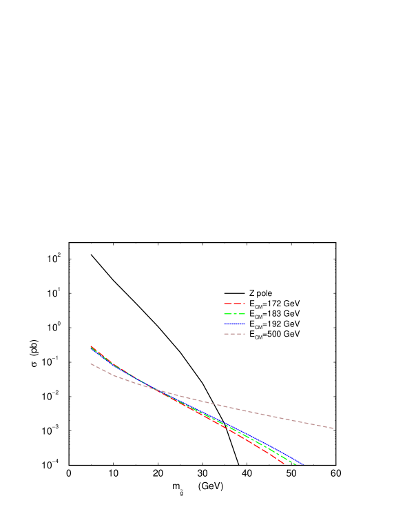
Figure 13: $\sigma(e^{+}e^{-}\to q\overline{q}\widetilde{g}\widetilde{g})$ as a function of $m_{\widetilde{g}}$ for $\sqrt{s}=m_{Z}$ (solid), 172 GeV (dashes), 183 GeV (dot-dash), 192 GeV (dots) and $500~{}{\rm GeV}$. No cuts.

Figure 14: Distributions of the number of $\widetilde{g}$-jets as a function of $\beta$ at LEP ($\sqrt{s}=m_{Z}$) for $m_{\widetilde{g}}=5$ and $25~{}{\rm GeV}$. No cuts are imposed.

Thus, we focus on $\sqrt{s}=m_{Z}$. The procedures for employing LEP $Z$-pole data to place constraints on the $\widetilde{g}$-LSP scenario depend upon the manner in which the $\widetilde{g}$-jet is manifested in the detector; this was outlined in the previous section. Generally speaking, $q\overline{q}\widetilde{g}\widetilde{g}$ events will have 4 jets and missing momentum. As noted in the previous section, the most crucial kinematical aspect of the $\widetilde{g}$-jets is their distribution as a function of $\beta$. The number of $\widetilde{g}$-jets as a function of $\beta$ is presented in Fig. 14 for $m_{\widetilde{g}}=5~{}{\rm GeV}$ and $25~{}{\rm GeV}$. We see that a light gluino with $m_{\widetilde{g}}\mathrel{\raise 1.29167pt\hbox{$<$\kern-7.5pt\lower 4.30554pt\hbox{$\sim$}}}5~{}{\rm GeV}$ has a $\beta$ distribution that peaks at $\beta\sim 0.98$ while a heavier gluino with $m_{\widetilde{g}}\sim 25~{}{\rm GeV}$ has a broad $\beta$ peak centered about $\beta\sim 0.6$, with the most probable $\beta$ values lying between $0.5$ and $0.7$. The implications of these $\beta$ ranges at these two masses were already indicated in the previous section. The reason that we will not be able to obtain limits from LEP data for very small $m_{\widetilde{g}}$ values is that as the gluino bound state mass decreases below $5~{}{\rm GeV}$, the initial $\beta$ of the $\widetilde{g}$ increases. As a result, the energy loss in the first few hadronic collisions increases significantly. For a mass of $\mathrel{\raise 1.29167pt\hbox{$<$\kern-7.5pt\lower 4.30554pt\hbox{$\sim$}}}1~{}{\rm GeV}$, the energy loss is essentially complete (that is the calorimeters will contain the hadron).

The most relevant LEP experimental analyses currently available are those related to the search for pair production of neutralinos, $Z\to\widetilde{\chi}^{0}_{1}\widetilde{\chi}^{0}_{2}$, with $\widetilde{\chi}^{0}_{2}\to q\overline{q}\widetilde{\chi}^{0}_{1}$. The OPAL [33] and L3 [34] analyses have the highest statistics and place limits on $\widetilde{\chi}^{0}_{1}\widetilde{\chi}^{0}_{2}$ production in the ${\rm jets}+/\hskip-8.0ptp_{T}$ channel that are potentially relevant for the $q\overline{q}\widetilde{g}\widetilde{g}$ final state. However, the L3 analysis is restricted entirely to $2j+/\hskip-8.0ptp_{T}$ final states. Only the OPAL analysis is relevant to any $nj+/\hskip-8.0ptp_{T}$ final state with $n\geq 2$. Typically, $q\overline{q}\widetilde{g}\widetilde{g}$ events give $n=2$, 3, or 4, depending upon the amount of energy deposition by the $\widetilde{g}$-jets.

The OPAL analysis is based on dividing the event into two hemispheres as defined by the thrust direction of the visible jets. We have implemented their procedures in a parton-level Monte Carlo and computed the efficiency for the $Z\to q\overline{q}\widetilde{g}\widetilde{g}$ events to pass their cuts as a function of $m_{\widetilde{g}}$ for various choices of the charged fragmentation probability $P$. Our precise procedures are as follows. In the OPAL analysis of multi-jet events, each event is divided into two hemispheres by the plane normal to the thrust axis, where the thrust $T$ is defined as

$$T={\rm max}_{\hat{n}}\frac{\sum_{i}|\vec{p}_{i}\cdot\hat{n}|}{\sum_{i}|\vec{p}_{i}|}$$ (15)

and the thrust axis is the $\hat{n}$ that leads to the maximum. In the OPAL analysis, the $\vec{p}_{i}$ are assigned to calorimeter clusters and associated tracks as described in the previous section. Associated energies are computed as if the track/cluster composites have very small mass. The sum of the (visible) four-momenta in a given hemisphere defines the four-momentum of the ‘jet’ associated with that hemisphere; note that the ‘jet’ need not have zero invariant mass. OPAL then separates events into mono- or di-‘jet’ events, where a mono-‘jet’ event is one having a ‘jet’ in only one hemisphere. Mono-‘jet’ events are discarded. The following cuts are then applied to the di-‘jet’ events:

where $(\pi-\theta_{\rm acol})$ is the three-dimensional angle between the two ‘jet’s, $(\pi-\theta_{\rm acop})$ is the angle between the two ‘jet’s in the $x$-$y$ plane, $\theta_{\rm miss}$ is the polar angle of the missing momentum, $M_{\rm vis}$ is the visible mass, and $\vec{p}$ (used to compute $p_{z}$ and $p_{T}$) is the vector sum of all (visible) three momenta. In the above, $M_{\rm vis}^{2}$ is computed by summing all the visible four-momenta (as defined earlier) in the event and taking the square. The square of $M_{\rm vis}^{\rm hem.}$ for each hemisphere is computed by summing the visible four-momenta in the hemisphere and squaring. The thrust, $T_{\rm hem.}$, for each hemisphere is defined by going to the center-of-mass for that hemisphere (defined by the sum of all visible three-momenta in the hemisphere being zero) and computing the thrust as in Eq. (15) using only the three-momenta of that hemisphere.

In applying the above procedures to the Monte Carlo events, it is necessary to adopt an algorithm for including the effects of detector resolution. In our computations, all cluster/track momenta and energies are smeared using the stated OPAL hadronic calorimeter energy resolution of $\Delta E/E=120\%/\sqrt{E(~{}{\rm GeV})}$. We note that energy smearing is important in that it generally increases the OPAL acceptance efficiencies by virtue of the fact that, on average, jet-energy mismeasurement tends to enhance the amount of missing momentum. This enhancement is especially important for $m_{\widetilde{g}}$ and $P$ choices (e.g. $m_{\widetilde{g}}=25~{}{\rm GeV}$ and $P=1$) such that the missing momentum before smearing is small. Another important ingredient is properly accounting for the fact that the $R$-hadron does not take the entire momentum of the $\widetilde{g}$. We have employed the standard Peterson [35] form for the fragmentation function of $\widetilde{g}\to R$:

$$D_{\widetilde{g}}^{R}=Cz^{-1}\left[1-{1\over z}-{\epsilon_{\widetilde{g}}\over 1-z}\right]^{-2}\,,$$ (17)

where we will take $\epsilon_{\widetilde{g}}=(0.3~{}{\rm GeV}/m_{\widetilde{g}})^{2}$. Here, the $R$-hadron carries a fraction $z$ of the momentum of the $\widetilde{g}$ and a normal (light quark or gluon) jet carries the remainder. The $R$-hadron is then treated in the calorimeter as we have described in the previous section. The energy of the remainder (effectively zero-mass) jet is taken equal to its momentum and is assumed to be entirely deposited in the calorimeter. Typically, fragmentation does not have a large influence on the efficiency with which events are retained, especially in cases for which the $\widetilde{g}$-jet energy is measured to be a large fraction of the $\widetilde{g}$’s initial kinetic energy.

The OPAL data corresponds to $N_{\rm had}=4.4\times 10^{6}$ hadronic $Z$ decays. The expected number of $q\overline{q}\widetilde{g}\widetilde{g}$ events after cuts is then

$$N={N_{\rm had}BR(Z\to q\overline{q}\widetilde{g}\widetilde{g})\times\mbox{efficiency}\over BR(Z\to{\rm hadrons})}\,,$$ (18)

where we use the efficiency as computed via the Monte Carlo. After cuts, OPAL observes 2 events with an expected background of $B=2.3$ events. The 95% upper limit on a possible new physics signal is then $S=4$ events, corresponding to $BR(Z\to q\overline{q}\widetilde{g}\widetilde{g})\times\mbox{efficiency}\sim 6.4\times 10^{-7}$. How low a value of $m_{\widetilde{g}}$ can be eliminated depends upon the efficiency at low $m_{\widetilde{g}}$. Because of the very high raw event rate at low $m_{\widetilde{g}}$ values, quite small efficiency can be tolerated. We will see that we can exclude gluino masses above $3-4~{}{\rm GeV}$.

Figure 15: In the upper window, we plot the OPAL $q\overline{q}\widetilde{g}\widetilde{g}$ event efficiency (after all cuts) in the $P=0,1/4,1/2,3/4,1$ cases, as computed using event-by-event determination of $E_{\rm jet}$ [using Eq. (14)] for each $\widetilde{g}$. For $P\neq 0,1$, changes of the $R$-hadron charge as it passes through the detector are randomly implemented. Both smearing and fragmentation effects are included. The lower window gives, as a function of $m_{\widetilde{g}}$, the corresponding 95% CL upper limits compared to the theoretical prediction for $BR(Z\to q\overline{q}\widetilde{g}\widetilde{g})$. Results are for the SC1 choices of $\lambda_{T}=19$ cm and $\langle\Delta E\rangle$ case (1).

As described in the previous section, to obtain a reliable result for the range of $m_{\widetilde{g}}$ that the OPAL analysis excludes, we have computed the efficiency for $q\overline{q}\widetilde{g}\widetilde{g}$ events to pass the full set of cuts when Eq. (14) is employed for each $\widetilde{g}$ on an event-by-event basis, including (for $P\neq 0,1$) random changes (with probability determined by $P$) of the $R$-hadron charge at each of the hadronic interactions it experiences as it passes through the detector. We have considered the three scenarios — SC1, SC2, and SC3 — for choices of $\lambda_{T}$ and the $\langle\Delta E\rangle$ case that were outlined at the end of the previous section. In Fig. 15, we plot the resulting OPAL efficiency for $q\overline{q}\widetilde{g}\widetilde{g}$ events after all cuts as a function of $m_{\widetilde{g}}$ for $P=0,1/4,1/2,3/4,1$ for the SC1 choices, including calorimeter energy smearing and fragmentation effects. Also shown are the resulting 95% CL upper limits on $BR(Z\to q\overline{q}\widetilde{g}\widetilde{g})$. We see that for any $P$ not near 1, the entire range from low $m_{\widetilde{g}}\sim 3~{}{\rm GeV}$ to high $m_{\widetilde{g}}\sim 25~{}{\rm GeV}$ is unambiguously excluded. For $P\sim 1$, the largest value of $m_{\widetilde{g}}$ that can be excluded is about $23~{}{\rm GeV}$. [The $m_{\widetilde{g}}\mathrel{\raise 1.29167pt\hbox{$>$\kern-7.5pt\lower 4.30554pt\hbox{$\sim$}}}23~{}{\rm GeV}$ limit for $P=1$ is similar to, but somewhat higher than, the limit obtained by searching for heavily-ionizing tracks at OPAL (discussed later in section 6).]

Figure 16: 95% CL upper limits as in Fig. 15 except that we do not include the effects of energy smearing or fragmentation.

In Fig. 16 we present the 95% CL limits obtained without including either energy smearing or Peterson fragmentation. This figure shows that the limits are little altered except for $P\sim 1$, in which case the OPAL analysis does not exclude any significant range of $m_{\widetilde{g}}$. It is energy smearing that is the dominant factor in obtaining a significant efficiency for event acceptance when $P\sim 1$. Even though $P\sim 1$ leads to $E_{\rm jet}\sim p_{\rm true}$ at the parton level [for the $\beta$ values typical for the $m_{\widetilde{g}}=5-25~{}{\rm GeV}$ mass range (see Fig. 12)] and thus small missing momentum at the parton level, energy smearing produces large event-by-event fluctuations in the measured energy of each $\widetilde{g}$ jet which lead to substantial missing momentum for many events.

Figure 17: 95% CL upper limits as in Fig. 15 except that we use the SC2 choices of $\lambda_{T}=9.5$ cm and $\langle\Delta E\rangle$ case (1) in the upper window and the SC3 choices of $\lambda_{T}=38$ cm and $\langle\Delta E\rangle$ case (2) in the lower window.

Results analogous to those obtained for the SC1 choices of $\lambda_{T}=19$ cm and $\langle\Delta E\rangle$ case (1), and presented in Fig. 15, are presented for the SC2 and SC3 choices [SC2: $\lambda_{T}=9.5$ cm, $\langle\Delta E\rangle$ case (1). SC3: $\lambda_{T}=38$ cm, $\langle\Delta E\rangle$ case (2)] in Fig. 17. In fact, these possible extremes always give higher efficiencies and a slightly larger range of $m_{\widetilde{g}}$ exclusion than found in the SC1 case.

We expect that re-analysis of the LEP data sets using cuts more appropriate to the $q\overline{q}\widetilde{g}\widetilde{g}$ final state for given values of $P$ and $m_{\widetilde{g}}$ will yield only a small improvement over the results obtained using the existing $\widetilde{\chi}^{0}_{1}\widetilde{\chi}^{0}_{2}$ analysis cuts. At large $m_{\widetilde{g}}$, the event rates are falling so rapidly that the 95% CL upper limit is not likely to be increased by more than a few GeV. Ruling out $m_{\widetilde{g}}$ values significantly below $3-5~{}{\rm GeV}$ will be difficult since for such $m_{\widetilde{g}}$ the gluino looks so much like a normal jet that only the still controversial analyses of Ref. [2] are likely to prove relevant. Still, we would recommend attempting to make use of the threshold in the mass recoiling against the two energetic jets of the the event present at $M_{\rm recoil}\sim 2m_{\widetilde{g}}$. Perhaps the background could be reduced to zero by an appropriate set of cuts including one requiring $M_{\rm recoil}\mathrel{\raise 1.29167pt\hbox{$>$\kern-7.5pt\lower 4.30554pt\hbox{$\sim$}}}2m_{\widetilde{g}}$.

It is also worth nothing that the jet energy as computed using the OPAL procedure of Eq. (14) is often larger than the actual $\widetilde{g}$ energy for large $P$. This may be interesting at LEP, since there it is possible to compare the total measured or ‘visible’ energy associated with an event to the total center of mass energy. By summing the assigned energies of all jets, one would find events in which the total energy exceeds the center of mass energy when $P$ is near 1. Indeed, the above Monte Carlo generates a significant number of such events when $m_{\widetilde{g}}$ is small. To our knowledge, the LEP experimental groups have not analyzed their events in a manner that would be sensitive to such a discrepancy.

Finally, we briefly discuss $e^{+}e^{-}\to\widetilde{g}\widetilde{g}$ production via quark-squark loops. Again, only the existing $Z$-pole data might possibly yield a useful constraint. As discussed in Refs. [31, 28], even if the squarks are all completely degenerate, the $Z\to\widetilde{g}\widetilde{g}$ branching ratio can be non-zero by virtue of the top mass being much greater than the bottom mass. However, Ref. [28] finds $BR(Z\to\widetilde{g}\widetilde{g})<2\times 10^{-4}$ for all $m_{\widetilde{g}}$ if the common squark mass ($\widetilde{m}$) is above $\sim 200~{}{\rm GeV}$. The typical event would contain two back-to-back jets. But these would not generally have equal energy due to the fact that fluctuations would be substantial, especially if $P$ is in a range such that there would sometimes, and sometimes not, be a charged track identified as a muon contained in one or both of the jets. For small deposited energy per $\widetilde{g}$-jet, as typical for small $P$, the net apparent energy of the typical event would be below $m_{Z}$, possibly causing such events to be confused with the two-photon background. For large enough $P$ and smaller $m_{\widetilde{g}}$, many of the events would be anomalous in that the sum of their apparent energies would exceed $m_{Z}$. We are uncertain if any of the LEP analyses would have been sensitive to such events appearing at a level corresponding to $BR(Z\to\widetilde{g}\widetilde{g})\sim 1-2\times 10^{-4}$. In any case, the $\widetilde{g}\widetilde{g}$ event rate can be suppressed to an unobservable level simply by taking $\widetilde{m}$ sufficiently large. (Roughly, $BR(Z\to\widetilde{g}\widetilde{g})$ falls as $1/\widetilde{m}^{2}$.) Thus, no model-independent $m_{\widetilde{g}}$ limits from the $\widetilde{g}\widetilde{g}$ final state are possible.

5 Present and Future Tevatron Constraints from jets + $/\hskip-8.0ptp_{T}$

In the $\widetilde{g}$-LSP scenario, with all other SUSY particles taken to be much heavier, the only standard hadron-collider SUSY signal is ${\rm jets}+/\hskip-8.0ptp_{T}$. Current mSUGRA analyses of this channel do not apply since the $\widetilde{g}$ does not cascade decay ($\widetilde{g}\to q\overline{q}\widetilde{\chi}^{0}_{1},\ldots$) to additional jets. In the $\widetilde{g}$-LSP scenario, for a given value of $m_{\widetilde{g}}$, fewer hard jets are expected and the amount of missing momentum is typically smaller. Consequently, the limits that can be placed on $m_{\widetilde{g}}$ from Tevatron data will be weaker. Still, we will find that substantial constraints can be placed on the $\widetilde{g}$-LSP scenario using existing Tevatron data, and that even stronger constraints will arise from RunII data.

In assessing the ability of the Tevatron to discover or exclude a heavy $\widetilde{g}$-LSP, we have employed cuts that mimic those employed by CDF in analyzing RunI data in the ${\rm jets}+/\hskip-8.0ptp_{T}$ channel. CDF cuts [36, 37] are employed rather than D0 cuts [38] since the CDF jet-energy and $/\hskip-8.0ptp_{T}$ requirements are weaker than required in the D0 cuts. For the same integrated luminosity, weak cuts allow greater sensitivity to the heavy $\widetilde{g}$-LSP situation in which the most energetic jets come from gluons radiated from the initial state colliding partons. The precise CDF cuts used are those employed in Ref. [4]; they are designed to duplicate the experimental procedures of Ref. [36] to the extent possible in the context of a Monte Carlo simulation.

• LI: No (isolated) leptons with $E_{T}>10~{}{\rm GeV}$.

• MPT: $/\hskip-8.0ptp_{T}>60~{}{\rm GeV}$.

• NJ: There are $n(jets)\geq 3$ with $|\eta_{\rm jet}|<2$ and $E_{T}>15~{}{\rm GeV}$, using a coalescence cone size of $\Delta R=0.5$.

• Azimuthal separation requirements as follows:

  • J1MPT: $\Delta\phi(/\hskip-8.0ptp_{T},j_{1})<160^{\circ}$;

  • JMPT: $\Delta\phi(/\hskip-8.0ptp_{T},j(E_{T}>20~{}{\rm GeV}))>30^{\circ}$.

  These are designed, in particular, to reduce QCD jet mismeasurement background.

Events were generated using ISAJET-7.37 [39]. Each event was passed through a toy calorimeter with cells of size $\Delta\eta\times\Delta\phi=0.1\times 0.1$ extending out to $|\eta|=4$. Electromagnetic and hadronic resolutions of $15\%/\sqrt{E}$ and $70\%/\sqrt{E}$, respectively, were chosen to approximate those of CDF. The most important cut is the missing transverse momentum (MPT) cut. This is especially true at low $m_{\widetilde{g}}$. Typically only a small fraction of the events are retained after the MPT cut. The next most important cut is the jet-number (NJ) cut. Typically, for $P$ and $m_{\widetilde{g}}$ choices that give larger MPT cut acceptance, the NJ cut acceptance is smaller. At the higher $m_{\widetilde{g}}=140~{}{\rm GeV}$ mass, the cuts retain a larger fraction of events than at lower mass. (But, of course, the cross section is smaller at high mass.)

Figure 18: The $\beta$ distributions of the $\widetilde{g}$’s produced in $p\overline{p}\to\widetilde{g}\widetilde{g}$, before cuts, for $m_{\widetilde{g}}=40~{}{\rm GeV}$ and $m_{\widetilde{g}}=140~{}{\rm GeV}$, taking $\sqrt{s}=1.8~{}{\rm TeV}$.

Figure 19: In the top window, the $\beta$ distribution of the $\widetilde{g}$’s produced in $p\overline{p}\to\widetilde{g}\widetilde{g}$, before cuts, for $m_{\widetilde{g}}=100~{}{\rm GeV}$, taking $\sqrt{s}=1.8~{}{\rm TeV}$. In the lower three windows, distributions in $\beta$ after cuts are compared for $P=0$, 1/2 and 1.

In order to relate the Tevatron situation to the discussion of section 3, it is useful to present the $\beta$ distribution of the $\widetilde{g}$ for several $m_{\widetilde{g}}$ values. In Fig. 18, we present the $\beta$ distributions, before cuts, for $m_{\widetilde{g}}=40~{}{\rm GeV}$ and $140~{}{\rm GeV}$, i.e. values near the upper and lower ends of the interesting mass range. For $m_{\widetilde{g}}\leq 40$, $\beta$ is typically $\geq 0.95$; for $m_{\widetilde{g}}\sim 140~{}{\rm GeV}$, the $\beta$ distribution peaks near $\beta\sim 0.75$, with most events having $0.5\leq\beta\leq 0.9$. The $\beta$ distributions, both before and after cuts (taking $P=0$, 1/2 and 1), are given for $m_{\widetilde{g}}=100~{}{\rm GeV}$ in Fig. 19. Referring back to Fig. 11 and related comments, we see that in all cases the most probable $\beta$ values are such that the measured $E_{\rm jet}$ of most $\widetilde{g}$-jets will be much smaller than the true momentum, thereby leading to large missing momentum as defined in the analysis.

Figure 20: The $/\hskip-8.0ptp_{T}$ distribution (before cuts) for $p\overline{p}\to\widetilde{g}\widetilde{g}$ events at $\sqrt{s}=1.8~{}{\rm TeV}$ is illustrated for $m_{\widetilde{g}}=100~{}{\rm GeV}$ and $P=0$, 1/2 and 1.

The distribution in $/\hskip-8.0ptp_{T}$ that results is illustrated for $m_{\widetilde{g}}=100~{}{\rm GeV}$ in Fig. 20. There, we see a substantial tail with $/\hskip-8.0ptp_{T}>60~{}{\rm GeV}$ that is essentially independent of the choice of $P$. This independence of $P$ is due to the small dependence of the $\beta$ distribution on $P$ (as illustrated in Fig. 19) and to the CDF procedure in which events where one of the $\widetilde{g}$-jets looks muonic are discarded and no correction is applied to the calorimetric energy measurement for a retained $\widetilde{g}$-jet that contains a penetrating track.

Let us now turn to determining the limits on a $\widetilde{g}$-LSP from the CDF data. To do so, we compare the cross section for $\widetilde{g}\widetilde{g}$ pair production after cuts to the SM background expected by CDF. For the above CDF cuts and $\sqrt{s}=1.8~{}{\rm TeV}$, Ref. [36] quotes a background rate of 28.7 events for $L=19~{}{\rm pb}^{-1}$, corresponding to $\sigma_{B}=1.51~{}{\rm pb}$. (A background rate of 33 events is quoted for the very slightly different $\geq 3$ jet cuts of the final published CDF analysis, Ref. [37]; we prefer to stick to the cuts of Ref. [36].) The 95% CL lower limit on $m_{\widetilde{g}}$ is obtained when the signal rate declines below the $1.96\sigma$ level, corresponding to $\sigma_{S}\sim 553~{}{\rm fb}$ (after cuts). We note that this is about the same as the $\sigma_{S}\sim 614~{}{\rm fb}$ required for a $5\sigma$ signal at $L=0.1~{}{\rm fb}^{-1}$. This latter cross section level will be indicated on our figures. In RunII, systematic uncertainties in the background will very probably determine the limit of sensitivity. Indeed, the 95% CL and $5\sigma$ levels for $\sigma_{S}$ are much lower for $L\geq 2~{}{\rm fb}^{-1}$ than the $\sigma_{S}$ sensitivity limit defined by $S/B>0.2$ (i.e. $\sigma_{S}>302~{}{\rm fb}$). For instance, the 95% CL cross section upper limits would be $53.9~{}{\rm fb}$ ($15.2~{}{\rm fb}$) for $L=2~{}{\rm fb}^{-1}$ ($25~{}{\rm fb}^{-1}$), respectively. If systematics can be understood at a better than 20% level, then the limits that could be obtained from RunII using RunI cuts would improve substantially as compared to the $S/B>0.2$ level limits. Correspondingly, a $\widetilde{g}$-LSP signal with $S/B\sim 0.2$ would have a very high nominal $S/\sqrt{B}$. Clearly, optimization of the cuts and procedures can be expected to improve upon these first estimates of sensitivity at RunII.

Figure 21: The cross section (after cuts) in the ${\rm jets}+/\hskip-8.0ptp_{T}$ channel is compared to (a) the $5\sigma$ level for $L=0.1~{}{\rm fb}^{-1}$ (also roughly the 95% CL upper limit for $L=19~{}{\rm pb}^{-1}$) at $\sqrt{s}=1.8~{}{\rm TeV}$ and (b) the $S/B=0.2$ level at RunII ($L\geq 2~{}{\rm fb}^{-1}$, $\sqrt{s}=2~{}{\rm TeV}$) as a function of $m_{\widetilde{g}}$ for $P=0$. SC1 choices of $\lambda_{T}=19$ cm and $\langle\Delta E\rangle$ case (1) are employed.

Figure 22: The cross section (after cuts) in the ${\rm jets}+/\hskip-8.0ptp_{T}$ channel is compared to (a) the $5\sigma$ level for $L=0.1~{}{\rm fb}^{-1}$ (also roughly the 95% CL upper limit for $L=19~{}{\rm pb}^{-1}$) at $\sqrt{s}=1.8~{}{\rm TeV}$ and (b) the $S/B=0.2$ level at RunII ($L\geq 2~{}{\rm fb}^{-1}$, $\sqrt{s}=2~{}{\rm TeV}$) as a function of $m_{\widetilde{g}}$ for $P=1/2$, using event-by-event determination of the momentum (=energy) of each $\widetilde{g}$-jet (including the probabilistic treatment of charge-exchanges at each hadronic collision) in events such that neither $\widetilde{g}$-jet is “muonic” (see text). SC1 choices of $\lambda_{T}=19$ cm and $\langle\Delta E\rangle$ case (1) are employed.

Figure 23: The cross section (after cuts) in the ${\rm jets}+/\hskip-8.0ptp_{T}$ channel is compared to (a) the $5\sigma$ level for $L=0.1~{}{\rm fb}^{-1}$ (also roughly the 95% CL upper limit for $L=19~{}{\rm pb}^{-1}$) at $\sqrt{s}=1.8~{}{\rm TeV}$ and (b) the $S/B=0.2$ level at RunII ($L\geq 2~{}{\rm fb}^{-1}$, $\sqrt{s}=2~{}{\rm TeV}$) as a function of $m_{\widetilde{g}}$ for $P=3/4$, using event-by-event determination of the momentum (=energy) of each $\widetilde{g}$-jet (including the probabilistic treatment of charge-exchanges at each hadronic collision) in events such that neither $\widetilde{g}$-jet is “muonic” (see text). SC1 choices of $\lambda_{T}=19$ cm and $\langle\Delta E\rangle$ case (1) are employed.

Figure 24: The cross section (after cuts) in the ${\rm jets}+/\hskip-8.0ptp_{T}$ channel is compared to (a) the $5\sigma$ level for $L=0.1~{}{\rm fb}^{-1}$ (also roughly the 95% CL upper limit for $L=19~{}{\rm pb}^{-1}$) at $\sqrt{s}=1.8~{}{\rm TeV}$ and (b) the $S/B=0.2$ level at RunII ($L\geq 2~{}{\rm fb}^{-1}$, $\sqrt{s}=2~{}{\rm TeV}$) as a function of $m_{\widetilde{g}}$ for $P=1$, using event-by-event determination of the momentum (=energy) of each $\widetilde{g}$-jet in events such that neither $\widetilde{g}$-jet is “muonic” (see text). SC1 choices of $\lambda_{T}=19$ cm and $\langle\Delta E\rangle$ case (1) are employed.

In Figs. 21, 22, 23 and 24, we plot the cross section, $\sigma_{S}$, after cuts, as a function of $m_{\widetilde{g}}$ for $P=0$, $1/2$, $3/4$ and $1$, for the SC1 choices of $\lambda_{T}=19$ cm and $\langle\Delta E\rangle$ case (1). Also shown on these plots is the $L=0.1~{}{\rm fb}^{-1}$ $S/\sqrt{B}=5$ cross section level (which, as discussed above, is about the same as the 95% CL lower limit for $L=0.19~{}{\rm fb}^{-1}$). We see that, at 95% CL, current CDF analyses [36, 37] of the $L=19~{}{\rm fb}^{-1}$ data set require $m_{\widetilde{g}}\mathrel{\raise 1.29167pt\hbox{$>$\kern-7.5pt\lower 4.30554pt\hbox{$\sim$}}}150,130,130,140~{}{\rm GeV}$ for $P=0,1/2,3/4,1$, respectively, and that, for all $P$, $m_{\widetilde{g}}$ values are excluded from the upper limit all the way down to $\leq 20~{}{\rm GeV}$ at a very high CL. Note that the $130-150~{}{\rm GeV}$ lower limit on $m_{\widetilde{g}}$ obtained is substantially below the lower limit that RunI data places on $m_{\widetilde{g}}$ in a typical MSSM model. For easy comparison, Figs. 21, 22, 23 and 24 all show the cross section (after cuts) resulting from gluino pair production in the MSSM model considered in Ref. [36] with $m_{\widetilde{q}}=1000~{}{\rm GeV}$, $\mu=-400~{}{\rm GeV}$ and $\tan\beta=4$; one sees that RunI data yields a 95% CL limit of roughly $m_{\widetilde{g}}\mathrel{\raise 1.29167pt\hbox{$>$\kern-7.5pt\lower 4.30554pt\hbox{$\sim$}}}210~{}{\rm GeV}$.

We re-emphasize that in the Monte Carlo we have treated each $\widetilde{g}$-jet on an event-by-event basis. In this way, the decision as to whether a given $\widetilde{g}$-jet is “muonic” is made event-by-event, including (for $P<1$) the possibility of charge changes (allowed for in random fashion on an event-by-event basis according to the chosen $P$) at each hadronic interaction as the $\widetilde{g}$ traverses the detector.

Figure 25: As in Fig. 23, except that SC2 choices of $\lambda_{T}=9.5$ cm and $\langle\Delta E\rangle$ case (1) are employed.

Figure 26: As in Fig. 23, except that SC3 choices of $\lambda_{T}=38$ cm and $\langle\Delta E\rangle$ case (2) are employed.

Figure 27: As in Fig. 24, except that SC2 choices of $\lambda_{T}=9.5$ cm and $\langle\Delta E\rangle$ case (1) are employed.

Figure 28: As in Fig. 22, except that SC3 choices of $\lambda_{T}=38$ cm and $\langle\Delta E\rangle$ case (2) are employed.

As for the OPAL analysis, we wish to assess sensitivity of our CDF results to the choices of $\lambda_{T}$ and $\langle\Delta E\rangle$ case. In order to do so we present several results for the extreme choices defined earlier in section 3, and denoted by scenario labels SC2 and SC3. First, in Figs. 25 and 26, we present $P=3/4$ results for the SC2 and SC3 choices, respectively. We observe that when $P$ is large SC2 (SC3) choices result in stronger (much weaker) limits from the CDF analysis. The poor SC3 results are easily understood as follows. For the SC3 choices, significantly less energy is deposited by a $\widetilde{g}$-jet. (The hadronic energy losses are smaller for the longer $\lambda_{T}$ and smaller case (2) $\langle\Delta E\rangle$’s, and the ionization energy losses are smaller because the $\widetilde{g}$ does not slow down as much due to the smaller hadronic energy losses.) As a result, when $P$ is large the $\widetilde{g}$-jet is much more likely to be declared to be “muonic”, both because it is highly probable that it will make it to either the inner or outer muon chamber, and be charged therein, and also because the total energy deposit will not exceed the CDF cutoff and thereby prevent its being declared to be a “muonic” jet. Thus, many more events are discarded. As $P$ increases above 3/4, the cross section obtained for a given $m_{\widetilde{g}}$ after cuts decreases further. For example, for $P=1$ current CDF jets + missing momentum data and analysis procedures provide no constraints on $m_{\widetilde{g}}$ for the SC3 choices, whereas Fig. 27 shows that strong constraints are provided for the SC2 choices. Finally, in Fig. 28, we show that, for $P=1/2$ (and smaller), even if we make the SC3 choices the limits on $m_{\widetilde{g}}$ are nearly as strong as for the SC1 choices of Fig. 22. For SC2 choices, the corresponding plot would show even stronger limits than for the SC1 choices.

Thus, the jets + missing momentum data and analysis of CDF only allows a $\widetilde{g}$ with $m_{\widetilde{g}}\leq 130~{}{\rm GeV}$ if the $\widetilde{g}$ has a high charged-fragmentation probability and rather weak hadronic interactions. Fortunately, the CDF heavily-ionizing-track analysis discussed later provides strong constraints for large $P$ that exclude this possibility for $m_{\widetilde{g}}\geq 50~{}{\rm GeV}$ (which should be extendable to lower $m_{\widetilde{g}}$ values). As we have repeatedly noted, the lack of sensitivity of the RunI CDF jets + missing momentum analysis would disappear if the data is re-analyzed without eliminating events containing a muonic jet. We urge the CDF collaboration to perform this re-analysis.

As one possible backup at low $m_{\widetilde{g}}$, we looked at whether or not UA1 [40] and UA2 [41] data could be used to exclude $m_{\widetilde{g}}$ in the $m_{\widetilde{g}}\sim 30~{}{\rm GeV}$ region. We find, however, that no limits on $m_{\widetilde{g}}$ in this (or any other mass region) are possible from the UA1 and UA2 data. Another backup at low $m_{\widetilde{g}}$ could be an analysis of pre-scaled data (i.e. data not taken at the full trigger rate) accumulated using lower $p_{T}$ cuts on the jets. For example, CDF took about $1~{}{\rm pb}^{-1}$ of data using a low-$E_{T}$ four-jet trigger [42]. Such data might be useful since at lower $m_{\widetilde{g}}$ the standard CDF cuts employed above tend to yield a rather small efficiency for accepting signal events. We have not examined this data in detail.

Let us now consider RunII. Returning to Figs. 21, 22, 23 and 24, we see that the limits based on $S/B>0.2$ will rise to $m_{\widetilde{g}}\geq 180,160,160,180~{}{\rm GeV}$ for $P=0,1/2,3/4,1$, respectively, for RunII (with $L>0.5~{}{\rm fb}^{-1}$). If systematics could be controlled so that a signal with $S/B\mathrel{\raise 1.29167pt\hbox{$<$\kern-7.5pt\lower 4.30554pt\hbox{$\sim$}}}10\%$ becomes reliable, each of these lower limits would be increased by about $30~{}{\rm GeV}$. All these potential lower bounds are, of course, still substantially lower than the $m_{\widetilde{g}}$ lower bound that can be achieved in the reference MSSM model for the same $S/B$ criterion (e.g. $250~{}{\rm GeV}$ for $S/B>0.2$). It is worth noting that RunII limits will be much less sensitive to $\lambda_{T}$ and $\langle\Delta E\rangle$. As shown in Fig. 26, even the SC3 choices will allow exclusion of all $m_{\widetilde{g}}\mathrel{\raise 1.29167pt\hbox{$<$\kern-7.5pt\lower 4.30554pt\hbox{$\sim$}}}130~{}{\rm GeV}$.

We end by noting that if the squarks are not much heavier than the $\widetilde{g}$, then the $\widetilde{g}\widetilde{g}$ cross section at the Tevatron will be reduced due to negative interference effects in the $q\overline{q}\to\widetilde{g}\widetilde{g}$ amplitude from squark exchanges. However, the $gg\to\widetilde{g}\widetilde{g}$ amplitude is unaffected. Further, additional very prominent signals will emerge from squark production channels that will more than compensate. Thus, the approach of taking all other SUSY particles to be much heavier than the $\widetilde{g}$ can be expected to yield the most conservative limits for the $\widetilde{g}$-LSP models.

6 The OPAL signal for a charged gluino hadron

OPAL has searched [43] for $e^{+}e^{-}\to q\overline{q}\widetilde{g}\widetilde{g}$ events in which the $\widetilde{g}$’s fragment to a charged $R^{\pm}$ that traverses their two-meter radius tracking chamber. They look for events with an anomalous value for the ionization $dE/dx$ as compared to the momentum $|\vec{p}|$. Both quantities are measured in the tracking chamber. As a result, penetration of the track to the muon detectors is not required. After appropriate kinematical cuts and cuts on the region of the $dE/dx-|\vec{p}|$ plane accepted, there is only one candidate event. They convert this into a 95% CL limit on the number of signal events. To interpret this limit they compute the expected number of gluinos produced and accepted and multiply by the probability $P$ for $\widetilde{g}\to R^{\pm}$ fragmentation. They place 95% CL upper limits on $P$ as given in Table 1.

$m_{\widetilde{g}}$	1.5	2.3	3.0	5.0	10.0	15.0	20.0
$P^{\,\rm max}_{95\%~{}CL}$	0.37	0.20	0.14	0.06	0.13	0.33	1.03

Table 1: The OPAL 95% CL upper limit on the probability $P$ for $\widetilde{g}\to R^{\pm}$ fragmentation as a function of $m_{\widetilde{g}}$.

As always, it is important to keep in mind that if the $R^{\pm}$ decays to a neutral state of any kind with a lifetime shorter than $\sim 10^{-7}~{}\mbox{sec}$, then $P$ is effectively zero since the $R^{\pm}$ will decay before traversing the tracker. Assuming a sufficiently long lifetime for the $R^{\pm}$, the limits of Table 1 can be interpreted in the context of the model for $P$ described earlier. For $P=1$, $1/2$ and 1/4, one excludes $m_{\widetilde{g}}=1-20~{}{\rm GeV}$, $1.2-16.6~{}{\rm GeV}$ and $1.9-13.6$, respectively. We have already seen that the OPAL jets plus missing momentum analysis excludes $m_{\widetilde{g}}=3-25~{}{\rm GeV}$ for any $P$ value not too close to 1; for $P\sim 1$, the upper limit declines to $\sim 23~{}{\rm GeV}$. Thus, the limits from our analysis of the OPAL jets plus missing momentum channel are nicely complementary to the OPAL heavily-ionizing track limits; they confirm one another for a substantial range of $m_{\widetilde{g}}$.

7 The CDF signal for a penetrating charged gluino hadron

The strength of this signal depends on the model used for gluino interactions and upon details of the detector. CDF’s central muon system consists of two muon detection scintillators separated by iron. To be identified as a penetrating charged particle, a particle must (a) penetrate the iron, (b) be charged at the scintillator layer just before it enters the iron and (c) be charged at the exit detection layer. To be identified as a heavily-ionizing particle, the particle must also be charged as it exits from the primary interaction and its ionization must be clearly larger than minimal.

Let us recall the picture we shall employ for the gluino as it traverses the detector. As in the OPAL analysis, the primary produced $\widetilde{g}$ is assumed to have some probability $P$ to fragment (immediately) to a charged $R^{\pm}$-hadron. The ionization of the $R^{\pm}$ will be measured shortly after emerging from the interaction vertex. The $R^{\pm}$ then undergoes a certain number of hadronic interactions as it passes through the calorimeters before arriving at the inner muon detection layer preceding the iron. As described earlier, we imagine that at each hadronic interaction the light quark’s and/or gluons are stripped from the $R$-hadron (whether neutral or charged at the time) leaving the bare gluino which then has the same probability $P$ to again become charged. Thus, the probability that the $R$-hadron is charged just before entering the muon iron is again $P$. As it traverses the iron it will undergo several more hadronic interactions and so the probability that it exits as a charged $R$-hadron is once again $P$. Altogether, we must reduce the cross section (after cuts to be discussed below) by $P^{3}$. Once again, this assumes that all the possible charged $R$-hadron states are effectively stable as they travel through the detector. If they decay rapidly to the $R^{0}$ or another neutral state, then this must be taken into account by an appropriate reduction of $P$.

Figure 29: The effective cross section $\sigma_{\rm eff}$ for one or more $\widetilde{g}$ to pass the heavily-ionizing penetrating particle cuts of Eqs. (19) and (LABEL:recon), including the efficiencies quoted in the text.

Whatever the value of $P$, we compute the event acceptance efficiency as follows [44]. For a given $m_{\widetilde{g}}$, we generate events using ISAJET. We impose the triggering requirement that at least one of the $\widetilde{g}$’s has

$$|\eta|<0.6~{}\mbox{and}~{}p_{T}>15~{}{\rm GeV}\,.$$ (19)

An efficiency of 0.8 is included for triggering on such a $\widetilde{g}$. We next demand that at least one of the $\widetilde{g}$’s satisfy the following heavily-ionizing, stable charged particle ‘reconstruction’ requirements:

We note that the $\beta\gamma<0.7$ requirement we impose for $m_{\widetilde{g}}<100~{}{\rm GeV}$ is such that only events in which ionization is at least three times minimal (as compared to twice minimal if only $\beta\gamma<0.85$ is required) are accepted. This cut is stronger than that of the actual analysis [44]. We do this in the hope that the background will be even smaller than the conservative number used later. In the above, we use $\beta_{\rm min}$ as given by the solid curve in Fig. 9. For $P$ substantially smaller than 1, this is quite conservative given that ionization energy loss will be much less than that employed in the figure, which is for $P=1$. Also, because we use $\beta_{\rm min}$ for $P=1$ and because typical $\beta$ values are substantially above $\beta_{\rm min}$, this analysis is quite insensitive to the choices of $\lambda_{T}$ and $\langle\Delta E\rangle$ case. Finally, an efficiency of 0.5 is included for the reconstruction. Note that one $\widetilde{g}$ could provide the trigger but fail the reconstruction while the other $\widetilde{g}$ could pass the reconstruction cuts. In Fig. 29 we plot the effective cross section $\sigma_{\rm eff}$ as a function of $m_{\widetilde{g}}$ after including the above cuts and efficiencies, but before including $P^{3}$. We note that no events pass the cuts for $m_{\widetilde{g}}<50~{}{\rm GeV}$; the cuts would have to be weakened, which might result in the introduction of substantial background.

Figure 30: The 95%CL upper limit on the probability $P$ for a $\widetilde{g}$ to fragment to a singly-charged $R^{\pm}$ hadron after production and collision is given as a function of $m_{\widetilde{g}}$ for $N_{B}=0$ and 10 background events.

In Ref. [25], it is stated that there are zero background events in $L=90~{}{\rm pb}^{-1}$ of data after the mass $>100~{}{\rm GeV}$ cuts. The background level probably increases gradually as one lowers the $m_{\widetilde{g}}$ value considered down to $50~{}{\rm GeV}$. (Current cuts do not allow sensitivity below this.) However, even for the less stringent $\beta\gamma<0.85$ cut the background level is estimated at $<12$ events [45] for $m_{\widetilde{g}}=50~{}{\rm GeV}$. To illustrate the situation, let us consider the cases of $N_{B}=0$ and 10 background events. At 95% CL we require $LP^{3}\sigma_{\rm eff}<3$ ($N_{B}=0$) or $<7$ ($N_{B}=10$). The resulting 95% CL upper limits on $P$ are plotted as a function of $m_{\widetilde{g}}$ in Fig. 30. We see that the limits on $P$ are significant. In particular, for $m_{\widetilde{g}}\sim 50~{}{\rm GeV}$ and $N_{B}\sim 10$, we find that $P>0.09$ is excluded. For $m_{\widetilde{g}}\sim 100~{}{\rm GeV}$ and $N_{B}=0$, $P>0.1$ is ruled out, rising to $P>0.2$ for $m_{\widetilde{g}}\sim 150~{}{\rm GeV}$. For $m_{\widetilde{g}}\geq 50~{}{\rm GeV}$, this result confirms the RunI jets+$/\hskip-8.0ptp_{T}$ analyses that exclude values of $m_{\widetilde{g}}$ below $130-150~{}{\rm GeV}$ down to $<20~{}{\rm GeV}$ for any $P$ for SC1 $\lambda_{T}$ and $\langle\Delta E\rangle$ case choices. The heavily-ionizing track signal improves (though only slightly) for SC3 choices, and thus excludes $m_{\widetilde{g}}\geq 50~{}{\rm GeV}$ (up to very big values) for $P\geq 1/2$ (i.e. for $P$ values such that the jets+$/\hskip-8.0ptp_{T}$ signal fails for the SC3 choices). We expect that, at large $P$, a CDF heavily-ionizing track analysis with weakened cuts would probably be able to extend the excluded $m_{\widetilde{g}}$ range down to the OPAL $m_{\widetilde{g}}\sim 22-25~{}{\rm GeV}$ lower bound (that applies for any $P$) based on the OPAL jets+$/\hskip-8.0ptp_{T}$ analysis and probably also down to the $\sim 20~{}{\rm GeV}$ bound (that applies for large $P$) from the OPAL heavily-ionizing track search. In any case, currently the only significant window for a $\widetilde{g}$-LSP in the $P$–$m_{\widetilde{g}}$ parameter space arises for SC3 choices and $P\mathrel{\raise 1.29167pt\hbox{$>$\kern-7.5pt\lower 4.30554pt\hbox{$\sim$}}}3/4$. The window at $P\sim 3/4$ is $25~{}{\rm GeV}\leq m_{\widetilde{g}}\leq 50~{}{\rm GeV}$, widening to $23~{}{\rm GeV}\leq m_{\widetilde{g}}\leq 50~{}{\rm GeV}$ for $P\sim 1$.

8 A gluino NLSP decaying to gluon plus gravitino

For completeness, we consider the scenario in which the gluino is not the LSP, but rather the NLSP (next-to-lightest supersymmetric particle), with the gravitino ($\widetilde{G}$) being the (now invisible) LSP. Such a situation can arise in GMSB models, including that of Ref. [5]. In this scenario, the gluino decays via $\widetilde{g}\to g\widetilde{G}$. Early universe/rare isotope limits are then irrelevant. Further, the decay will be prompt from the detector point of view if $m_{\widetilde{G}}$ is in the $\leq$ few eV region such that the $\widetilde{G}$ is guaranteed to have no impact on $\Omega h^{2}$ [46, 47]. (If the scale of supersymmetry breaking is so large that the $\widetilde{g}\to g\widetilde{G}$ decay lifetime is long enough that most $\widetilde{g}$’s exit the detector before decaying, then the results of previous sections apply.) The first examination of this scenario at the Tevatron appears in Ref. [48]. We are unaware of any studies of this scenario for the $q\overline{q}\widetilde{g}\widetilde{g}$ final state at LEP or LEP2. Here, we will give the 95% CL excluded mass domains based on the previously considered jets + missing momentum analyses of OPAL [33] and CDF [36, 37]. In our analysis, we will assume that the branching ratio of $\widetilde{g}\to g\widetilde{G}$ is 100% (as appropriate if the $\widetilde{g}$ is the NLSP), and that the decay is prompt. We will also assume that the $\widetilde{G}$ has negligible mass compared to $m_{\widetilde{g}}$, and that other supersymmetric particles are much heavier than the gluino.

Figure 31: In the upper window, we plot the OPAL $q\overline{q}\widetilde{g}\widetilde{g}$ event efficiency (after all cuts) in the $\widetilde{g}\to g\widetilde{G}$ scenario. The lower window gives, as a function of $m_{\widetilde{g}}$, the corresponding 95% CL upper limits compared to the theoretical prediction for $BR(Z\to q\overline{q}\widetilde{g}\widetilde{g})$.

Consider first, the OPAL analysis. Using exactly the same procedures and cuts as discussed earlier in section 4, but applied to $e^{+}e^{-}\to Z\to q\overline{q}\widetilde{g}\widetilde{g}\to q\overline{q}gg+/\hskip-8.0ptp_{T}$, we have determined the efficiency for event acceptance and the resulting 95% CL upper limit on $BR(Z\to q\overline{q}\widetilde{g}\widetilde{g})$. These results appear in Fig. 31. Gluino masses below about $26~{}{\rm GeV}$ are clearly excluded.

Figure 32: The cross section (after cuts) in the ${\rm jets}+/\hskip-8.0ptp_{T}$ channel is compared to (a) the $5\sigma$ level for $L=0.1~{}{\rm fb}^{-1}$ (also roughly the 95% CL upper limit for $L=19~{}{\rm pb}^{-1}$) at $\sqrt{s}=1.8~{}{\rm TeV}$ and (b) the $S/B=0.2$ level at RunII ($L\geq 2~{}{\rm fb}^{-1}$, $\sqrt{s}=2~{}{\rm TeV}$) as a function of $m_{\widetilde{g}}$ for the $\widetilde{g}\to g\widetilde{G}$ case.

For our CDF-based analysis of the $\widetilde{g}\to g\widetilde{G}$ scenario we employ the same procedures as in section 5. We compute jets+$/\hskip-8.0ptp_{T}$ rates based on $p\overline{p}\to\widetilde{g}\widetilde{g}X$. The plots analogous to those given earlier appear in Fig. 32. We observe that the jets+$/\hskip-8.0ptp_{T}$ signal cross section (after cuts) for a $\widetilde{g}$-NLSP is even larger than in the reference MSSM model. All values of $m_{\widetilde{g}}\mathrel{\raise 1.29167pt\hbox{$<$\kern-7.5pt\lower 4.30554pt\hbox{$\sim$}}}240~{}{\rm GeV}$ (down to very small values that clearly overlap the OPAL exclusion region for this scenario) can be excluded at 95% CL based on the CDF $L=19~{}{\rm pb}^{-1}$ data sample analysis. This result is stronger than the bound obtained in Ref. [48]. The same CDF analysis procedures applied at RunII will be able to exclude $m_{\widetilde{g}}$ values up to about $280~{}{\rm GeV}$. Analyses optimized for such higher masses will presumably be able to do even better.

Overall, it is clear that a gluino NLSP decaying to gluon plus light gravitino can be excluded for essentially all $m_{\widetilde{g}}\mathrel{\raise 1.29167pt\hbox{$<$\kern-7.5pt\lower 4.30554pt\hbox{$\sim$}}}240~{}{\rm GeV}$.

9 Insights for other new physics analyses

In this section, we wish to emphasize a few interesting possibilities for other analyses for new physics that can be extracted from the lessons learned in our specific studies.

The primary point to note is that our results imply that the jets plus missing momentum signal is immediately applicable for pair production of any type of stable or semi-stable (i.e. stable within the detector) neutral or charged heavy particle that is produced via the strong interactions. Examples of such particles abound in the literature.

• Gauge-mediated supersymmetry breaking models can contain colored messengers in the gauge-mediation sector that are stable or semi-stable.

• In models with extra generations, one or more of the heavy quarks could be long-lived.

• Semi-stable, strongly-interacting massive particles are proposed as a source of ultra-high-energy cosmic ray events.

Pair production of a heavy stable particle produced via strong interactions gives rise to a substantial missing momentum signal due to the mismatch between the true momentum of each produced particle and the apparent energy of the jet associated with the particle (as measured after including calorimeter response and possible identification of any associated charged hadron track as a muon track within the jet). Further, the net missing momentum in a typical pair-production event does not tend to be aligned with the visible energy of the jet associated with any one of the heavy particles. This is because in a realistic Monte Carlo the pair-production process initiated by quarks and/or gluons in the colliding hadrons is accompanied by additional jets with high transverse momentum coming from initial state ‘radiation’.

In the case of pair production of heavy stable quarks at a hadron collider, the limits from the jets plus missing momentum analysis would be very complementary to the heavily-ionizing, penetrating track limits that rely more heavily on substantial modeling of the charge exchange and fragmentation for a heavy quark as it passes through the detector. As discussed earlier, the rate for the latter signals scales roughly as $P^{3}$, where $P$ is the probability for the heavy quark to fragment to a charged (as opposed to neutral) heavy hadron. For small enough $P$, the missing momentum signal will be stronger than the penetrating track signal. In addition, there is a very interesting hybrid signal that should be analyzed. A missing momentum trigger could be used to isolate events in which to look for a heavily-ionizing track. This could be more efficient than the present CDF analysis which requires a penetrating track in order to have a trigger rate such that all events can be accepted. The jets plus missing momentum trigger would eliminate the need to require a penetrating track and one could just search for a heavily-ionizing track in events accepted by the trigger. The advantage would be that the probability for the heavily-ionizing track (without requiring penetration) scales only as $P$ (rather than $P^{3}$).

It might be possible to take direct advantage of the mismatch between different ways of measuring the momentum of a heavy particle that is contained in a charged state after the initial interaction. The tracker would measure the true momentum of the particle. There are then two possibilities.

• If the additional tracks are not present that cause the track observed in the tracker to be deemed as having penetrated to the muon detector, then this true momentum could be directly compared to the momentum of the particle as determined by the calorimeter response. We have seen that there is generally a very substantial difference. This situation would have probability $\propto P(1-P^{2})$ (including the probability for the initial track in the tracker).

• Alternatively, if the track observed in the tracker is deemed to have penetrated to the muon detector, one could compare the true momentum to that computed for the jet assuming the track belonged to a muon [see Eq. (14)]. The difference is substantial when the average $\beta$ of the produced particle is large.

In order to retain as many events as possible it would be best to use a simple multi-jet trigger (without necessarily requiring missing momentum). Of course, since we are looking for momentum discrepancies for a single jet, it would be necessary to perform a very careful study of backgrounds, such as that due to jets that are mismeasured and/or fragment to $K_{L}^{0}$’s.

10 Summary and Conclusions

We have examined constraints on any model in which the gluino is the LSP. In section 2, we considered the relic cosmological density of a $\widetilde{g}$-LSP. We found that the relic density depends very strongly on the presence and nature of non-perturbative effects that could enter into the gluino and gluino-bound-state annihilation cross sections. Assuming a completely perturbative $\widetilde{g}\widetilde{g}$ annihilation cross section leads to a relic density of $\Omega h^{2}\sim(m_{\widetilde{g}}/10~{}{\rm TeV})^{2}$. For $m_{\widetilde{g}}\mathrel{\raise 1.29167pt\hbox{$>$\kern-7.5pt\lower 4.30554pt\hbox{$\sim$}}}100~{}{\rm GeV}$, this level of relic density is probably inconsistent with bounds from limits from heavy isotopes, underground detector interaction rates and the like. However, we found that non-perturbative effects can potentially decrease the relic density to $\Omega h^{2}\sim 10^{-10}$ for all $m_{\widetilde{g}}\mathrel{\raise 1.29167pt\hbox{$<$\kern-7.5pt\lower 4.30554pt\hbox{$\sim$}}}10~{}{\rm TeV}$, a level that would be entirely consistent with all constraints. Our conclusion is that, until the non-perturbative physics associated with gluino-gluino annihilation can be clarified, no reliable limits on the $\widetilde{g}$-LSP can be obtained from constraints requiring knowledge of its relic density. Thus, direct limits from accelerator experiments are of great interest.

In section 3, we studied the manner in which a (stable) $\widetilde{g}$-LSP is manifested in a typical detector. The critical issue for experimental analyses is the average amount of visible momentum assigned to a gluino jet. For a given detector, this depends upon many ingredients, including the average hadronic collision length of the $R$-hadron into which the $\widetilde{g}$ fragments, the average hadronic energy deposited in the various collisions experienced by the $R$-hadron as it passes through the detector, and the typical velocity and charge of the $R$-hadron. The hadronic collision length was estimated using the two-gluon model for total cross sections; one finds a collision length that is somewhat longer than for a typical light hadron. Collision lengths that are twice as large and one-half as large as our central prediction were also considered. Two cross section models were employed for computing the average energy deposit (as a function of velocity) in each hadronic collision. The (generally fluctuating) charge of the $R$-hadron as it passes through the detector is also a crucial ingredient and is characterized in terms of the probability $P$ for the $\widetilde{g}$ to turn into a stable charged $R^{\pm}$, such as $\widetilde{g}u\overline{d}$, as opposed to a neutral state, such as the $R^{0}=\widetilde{g}g$, after a hadronic collision. Simple quark counting models suggest $P<1/2$ and probably much smaller if the $\widetilde{g}g$ bound state is important. For $P=0$, the energy (=momentum) assigned to a gluino jet will be equal to the amount of the $\widetilde{g}$ kinetic energy that is deposited in the calorimeters due to hadronic collisions. For $P>0$, the ionization energy deposits must be included and the possible interpretation of an $R^{\pm}$ track in the central tracker as a muon within the $\widetilde{g}$-jet must be taken into account.

In order to do this properly in a Monte Carlo context, for any given value of $P$, the momentum measured for each $\widetilde{g}$ is computed on an event-by-event basis, including (for $P\neq 0,1$) random changes (according to the value of $P$) of the charge of the $R$-hadron at each hadronic collision as the $\widetilde{g}$ passes through the detector. Procedures are highly dependent upon the detector and specific analysis in question. For example, in the LEP OPAL jets + missing momentum analysis, if the $R$-hadron is an $R^{\pm}$ in the tracker and penetrates as an $R^{\pm}$ to the muon chamber, then the $\widetilde{g}$-jet is declared to contain a muon and a procedure for adding in the supposed muon track momentum (and correcting for its presumed minimal ionization energy deposit in the calorimeter) is followed. In contrast, in the CDF jets + missing momentum analysis for Tevatron RunI, if the $R$-hadron is an $R^{\pm}$ in the tracker and appears as an $R^{\pm}$ in one of the muon chambers, and if the net measured calorimeter energy is not too large, then the $\widetilde{g}$-jet is declared to be muonic and the event is discarded.

We studied the momentum typically assigned to the $\widetilde{g}$-jet as a function of $P$, for the $\widetilde{g}$ masses and velocities of relevance, in the OPAL and CDF analyses. For all $P$ (for $P\leq 1/2$), we found that the CDF (OPAL) procedure implies that the momentum assigned to the $\widetilde{g}$-jet is (on average) only a small fraction of its actual momentum unless $m_{\widetilde{g}}$ is smaller than a few GeV. This is true even for the cross section choice that overestimates energy deposits and even though, in the OPAL procedure, we allow for the appropriate fraction of cases (determined by $P$) in which the $\widetilde{g}$ penetrates to the muon chamber and has an $R^{\pm}$ track that is treated as a muon component of the jet in reconstructing the jet energy. Thus, when the $\widetilde{g}$ is the lightest supersymmetric particle, the jets plus missing momentum signature at colliders is, indeed, relevant. In fact, this would be the dominant standard SUSY signal if all other supersymmetric particles, in particular those with strong production cross sections, are significantly heavier than the $\widetilde{g}$.

Section 3 ended with a discussion of the effects of incomplete containment of a shower from a hadronic interaction that takes place near the outer edge of the hadronic calorimeter (or outer edge of uninstrumented iron). Effects, on the OPAL and CDF analyses summarized below, from the failure to include the shower energy in the measured jet energy and from the extra tracks in the subsequent muon-chamber(s) are outlined.

As noted, existing jets plus missing momentum analyses at both LEP and the Tevatron are relevant to excluding a range of $m_{\widetilde{g}}$ values in the $\widetilde{g}$-LSP scenario. In section 4, we demonstrated that the OPAL LEP data analysis that has been performed in order to search for $Z\to\widetilde{\chi}^{0}_{1}\widetilde{\chi}^{0}_{2}$ (with $\widetilde{\chi}^{0}_{2}\to q\overline{q}\widetilde{\chi}^{0}_{1}$) in the jets plus missing momentum channel can be applied to $Z\to q\overline{q}\widetilde{g}\widetilde{g}$ events. For $P=0,1/4,1/2,3/4$, we found that $m_{\widetilde{g}}$ values from $\sim 3~{}{\rm GeV}$ up to $\sim 25~{}{\rm GeV}$ are excluded at the 95% CL, for all choices of path length $\lambda_{T}$ and $\langle\Delta E\rangle$ energy loss (per hadronic collision) case considered. For $P=1$, and after including energy smearing and fragmentation effects, the upper limit of the excluded range declines to $m_{\widetilde{g}}\sim 23~{}{\rm GeV}$ for our standard or “SC1” choices of $\lambda_{T}$ and $\langle\Delta E\rangle$ case. There is almost no change of the excluded range of $m_{\widetilde{g}}$ for possible extreme choices of $\lambda_{T}$ and $\langle\Delta E\rangle$ (with scenario labels “SC2” and “SC3”). For the “SC1” choices, results for $P\sim 1$ are sensitive to whether or not we include energy smearing and fragmentation effects. If these effects are not included, the fluctuations in measured jet energy are reduced and no limit is possible for $P=1$ from OPAL jets + missing momentum data. (But, as discussed below, much the same range of $3\mathrel{\raise 1.29167pt\hbox{$<$\kern-7.5pt\lower 4.30554pt\hbox{$\sim$}}}m_{\widetilde{g}}\mathrel{\raise 1.29167pt\hbox{$<$\kern-7.5pt\lower 4.30554pt\hbox{$\sim$}}}20~{}{\rm GeV}$ is excluded by the heavily-ionizing track signal.) In contrast, for $P\leq 3/4$, the excluded range of $m_{\widetilde{g}}$ is essentially independent of whether or not energy smearing and fragmentation are included. Turning to LEP2, we noted that accumulated luminosities will not be adequate to improve the LEP $Z$-pole limits. A next linear collider operating at $\sqrt{s}=500~{}{\rm GeV}$ would be able to extend the LEP limits, but probably not beyond the limits that are imposed by our Tevatron analysis.

In section 5, we analyzed constraints from the Tevatron, assuming that all other SUSY particles are much heavier. We believe the resulting limits on $m_{\widetilde{g}}$ to be conservative. We examined the jets plus missing momentum channel using cuts and procedures based on the currently published CDF analysis of $L=19~{}{\rm pb}^{-1}$ of RunI data. The cross section limits obtained by CDF translate to a range of excluded $m_{\widetilde{g}}$ values. At 95% CL, we exclude $m_{\widetilde{g}}$ up to $\sim 130-150~{}{\rm GeV}$ (the precise upper limit depending on $P$) down to at least $20~{}{\rm GeV}$ (at a very high CL), for “SC1” or “SC2” choices of $\lambda_{T}$ and $\langle\Delta E\rangle$ case. For “SC3” choices (corresponding to long path length and small hadronic energy deposits per collision for the $\widetilde{g}$) the current CDF analysis can only exclude the above range of $m_{\widetilde{g}}$ for $P\leq 1/2$. Thus, for all but “SC3” choices, the CDF RunI limit overlaps the OPAL limit for any value of $P$, and all values of $m_{\widetilde{g}}$ in the $\sim 3~{}{\rm GeV}-130~{}{\rm GeV}$ range are excluded. For “SC3” $\lambda_{T}$ and $\langle\Delta E\rangle$ case choices, these same CDF limits apply only for $P\leq 1/2$. This lack of sensitivity of the CDF analysis at large $P$ to long $\lambda_{T}$ and/or small $\langle\Delta E\rangle$ could be eliminated by a re-analysis of the data that retains muonic jets.

RunII Tevatron data in the jets plus missing momentum channel can be expected to extend the exclusion region to higher masses; depending upon $P$, we found that roughly $m_{\widetilde{g}}\mathrel{\raise 1.29167pt\hbox{$<$\kern-7.5pt\lower 4.30554pt\hbox{$\sim$}}}160-180~{}{\rm GeV}$ will be excluded for “SC1” or “SC2” choices of $\lambda_{T}$ and $\langle\Delta E\rangle$ case. For “SC3” choices and high $P$, only $m_{\widetilde{g}}\mathrel{\raise 1.29167pt\hbox{$<$\kern-7.5pt\lower 4.30554pt\hbox{$\sim$}}}130~{}{\rm GeV}$ would be excluded. Such sensitivity is substantially worse than that found for the MSSM with mSUGRA boundary conditions, for which one can probe out to roughly $m_{\widetilde{g}}\mathrel{\raise 1.29167pt\hbox{$<$\kern-7.5pt\lower 4.30554pt\hbox{$\sim$}}}250~{}{\rm GeV}$. Possibly the RunII reach in the $\widetilde{g}$-LSP scenario could be extended if systematic errors are smaller than anticipated. The above limitation assumes that $S/B>0.2$ is required for a detectable signal. Alternative cuts, with smaller $B$ at high $m_{\widetilde{g}}$, might also yield a larger reach. Although we have not specifically performed the analysis, the Tevatron results suggest that the LHC can be expected to rule out a $\widetilde{g}$-LSP with $m_{\widetilde{g}}$ up to at least 1 TeV.

We also explored limits on a $\widetilde{g}$-LSP deriving from the non-observation of a pseudo-stable charged track which is heavily-ionizing. The strength of such signals depends on $P$. In section 6, we reviewed the OPAL results. OPAL performed a direct search for such states using cuts in the $dE/dx-|\vec{p}|$ plane, concluding that for $P\sim 1/2$ ($P\sim 1$) one can exclude $m_{\widetilde{g}}$ in the $\sim 1-17~{}{\rm GeV}$ ($\sim 1-20~{}{\rm GeV}$) mass range. For heavy-ionization signals at higher masses we must turn to the Tevatron. CDF looks for events containing a pseudo-stable penetrating charged track which is heavily-ionizing. In section 7, we demonstrated that, depending upon $P$, $\widetilde{g}$-pair production can lead to a significant cross section (after imposing the CDF cut, penetration and ionization requirements for identifying such events with small background). We have estimated the upper limit from RunI data on the probability $P$ of charged fragmentation of the $\widetilde{g}$. The upper limit can be roughly parameterized as $P\sim 0.3(m_{\widetilde{g}}/200~{}{\rm GeV})$ for $100\mathrel{\raise 1.29167pt\hbox{$<$\kern-7.5pt\lower 4.30554pt\hbox{$\sim$}}}m_{\widetilde{g}}\mathrel{\raise 1.29167pt\hbox{$<$\kern-7.5pt\lower 4.30554pt\hbox{$\sim$}}}250~{}{\rm GeV}$. For $m_{\widetilde{g}}<140~{}{\rm GeV}$, this means that $P<0.18$ is required. Meanwhile: the jets plus missing momentum limits based on OPAL and CDF analyses exclude $3~{}{\rm GeV}\mathrel{\raise 1.29167pt\hbox{$<$\kern-7.5pt\lower 4.30554pt\hbox{$\sim$}}}m_{\widetilde{g}}\mathrel{\raise 1.29167pt\hbox{$<$\kern-7.5pt\lower 4.30554pt\hbox{$\sim$}}}130-150~{}{\rm GeV}$ for $P\leq 1/2$; the OPAL jets plus missing momentum analysis excludes $\sim 3~{}{\rm GeV}\mathrel{\raise 1.29167pt\hbox{$<$\kern-7.5pt\lower 4.30554pt\hbox{$\sim$}}}m_{\widetilde{g}}\mathrel{\raise 1.29167pt\hbox{$<$\kern-7.5pt\lower 4.30554pt\hbox{$\sim$}}}25~{}{\rm GeV}$ for any $P$ not too near 1 ($\sim 3~{}{\rm GeV}\mathrel{\raise 1.29167pt\hbox{$<$\kern-7.5pt\lower 4.30554pt\hbox{$\sim$}}}m_{\widetilde{g}}\mathrel{\raise 1.29167pt\hbox{$<$\kern-7.5pt\lower 4.30554pt\hbox{$\sim$}}}23~{}{\rm GeV}$ for $P=1$); and, the CDF jets plus missing momentum analysis excludes $m_{\widetilde{g}}$ from $\sim 20~{}{\rm GeV}$ to $\sim 130~{}{\rm GeV}$ for $P=3/4$ and $P=1$ for all but “SC3” choices of $\lambda_{T}$ and $\langle\Delta E\rangle$ case. For $P\geq 1/2$ (independent of $\lambda_{T}$ and $\langle\Delta E\rangle$), the CDF heavily-ionizing track analysis excludes $50\leq m_{\widetilde{g}}\leq 200~{}{\rm GeV}$. This leaves only the possibility that “SC3’ choices apply, that $P$ lies in the (less likely) $P\mathrel{\raise 1.29167pt\hbox{$>$\kern-7.5pt\lower 4.30554pt\hbox{$\sim$}}}3/4$ range, and that $m_{\widetilde{g}}$ lies in the $\sim 23-50~{}{\rm GeV}$ window. Very probably, an extension of the CDF heavily-ionizing penetrating particle analysis with weakened cuts appropriate to these lower masses could exclude this window.

For completeness, in section 8 we also considered the scenario where the gluino is the NLSP (next-to-lightest supersymmetric particle) and the gravitino is the LSP. Such a situation is quite possible in models with gauge-mediated supersymmetry breaking. In this scenario, the gluino decays via $\widetilde{g}\to g\widetilde{G}$ and the $\widetilde{G}$ is invisible. There is then a strong jets+$/\hskip-8.0ptp_{T}$ signal at both LEP and the Tevatron. We repeated the LEP OPAL-based analysis and the $L=19~{}{\rm pb}^{-1}$ CDF-based analysis for this case and found that $m_{\widetilde{g}}\mathrel{\raise 1.29167pt\hbox{$<$\kern-7.5pt\lower 4.30554pt\hbox{$\sim$}}}240~{}{\rm GeV}$ can be excluded at 95% CL. RunII should be able to extend the excluded region to at least $m_{\widetilde{g}}\sim 280~{}{\rm GeV}$.

Finally, we urge our experimental colleagues to take note of our remarks in section 9 regarding the applicability of our procedures in the jets plus missing momentum channel, or hybrid procedures such as combining a jets plus missing momentum trigger with a heavily-ionizing track requirement, to placing limits on other exotic particles, such as a heavy stable quark. We also note that a search for heavily-ionizing tracks in events with jets plus missing momentum should prove very valuable for excluding $P>1/2$ $\widetilde{g}$-LSP scenarios.

11 Acknowledgements

This work was supported in part by the DOE under contracts No. DE-FG03-91ER40674 and No. DE-FG05-87ER40319, and in part by the Davis Institute for High Energy Physics. The hospitality of the Aspen Center for Physics, where this work was begun, is gratefully acknowledged. We would like to thank S. Brodsky, M. Drees, J. Kiskis, S. Mani, S. Raby and K. Tobe for helpful discussions. We are especially grateful to M. Albrow, H. Frisch, T. LeCompte, J. Hauser, S. Mani, D. Stuart and R. Van Kooten for extremely valuable discussions regarding the D0, CDF and OPAL detectors and algorithms, and for critical examination of our procedures for computing energy losses.

References

- [1] G.R. Farrar, Phys. Rev. Lett. 76 (1996) 4111,4115; Phys. Rev. 51 (1995) 3904. For a recent review, see G.R. Farrar, preprint RU-97-79 [hep-ph/9710277], to appear in the Proceedings of the 5th International Conference on Supersymmetries in Physics (SUSY 97), University of Pennsylvania, Philadelphia, PA, 27–31 May 1997, edited by M. Cvetic and P. Langacker.
- [2] F. Csikor and Z. Fodor, Phys. Rev. Lett. 78 (1997) 4335; preprint ITP-BUDAPEST-538 [hep-ph/9712269]; Z. Nagy and Z. Trocsanyi, hep-ph/9708343; hep-ph/9712385; J. Adams et al. [KTeV Collaboration], Phys. Rev. Lett. 79 (1997) 4083; P. Abreu et al. [DELPHI Collaboration], Phys. Lett. B414 (1997) 410; R. Barate et al. [ALEPH Collaboration], Z. Phys. C96 (1997) 1.
- [3] V.S. Kaplunovsky and J. Louis, Phys. Lett. B306 (1993) 269; A. Brignole, L.E. Ibanez and C. Munoz, Nucl. Phys. B422 (1994) 125, [E: B436 (1995) 747]; CERN-TH/97-143 [hep-ph/9707209].
- [4] C.H. Chen, M. Drees, and J.F. Gunion, Phys. Rev. 55 (1997) 330.
- [5] S. Raby, Phys. Rev. 56 (1997) 2852; hep-ph/9712254.
- [6] G.D. Starkman, A. Gould, R. Esmailzadeh and S. Dimopoulos, Phys. Rev. 41 (1990) 3594.
- [7] C.B. Dover, T.K. Gaisser and G. Steigman, Phys. Rev. Lett. 42 (1979) 1117.
- [8] S. Wolfram, Phys. Lett. 82B (1979) 65.
- [9] R.N. Mohapatra and S. Nussinov, Phys. Rev. D57 (1997) 1940.
- [10] J.F. Gunion, preprint UCD-98-2, Proceedings of of the International Workshop on Quantum Effects in the MSSM, UAB, Barcelona, September 9–13 1997, ed. J. Sola (World Scientific Publishing).
- [11] P. Gondolo and G. Gelmini, Nucl. Phys. B360 (1991) 145.
- [12] A. Sommerfeld, Ann. Phys. 11 1931 257; A.I. Akhiezer and V.B. Berestetsky, Quantum electrodynamics; J. Schwinger, Particles, Sources and Fields, Vol. II (Addison-Wesley), p. 397f.
- [13] T. Appelquist and H.D. Politzer, Phys. Rev. Lett. 34 (1975) 43.
- [14] S. Brodsky, J.F. Gunion and D.E. Soper, Phys. Rev. D36 (1987) 2710.
- [15] W. Beenakker, R. Hopker, M. Spira and P. Zerwas, Z. Phys. C69 (1995) 163.
- [16] J.L. Richardson, Phys. Lett. 82B (1979) 272.
- [17] H. Baer, K. Cheung, J.F. Gunion and J.E. Kiskis, work in progress.
- [18] J.F. Gunion and D.E. Soper, Phys. Rev. D15 (1977) 2617.
- [19] K. Griest and M Kamionkowski, Phys. Rev. Lett. 64 (1990) 615.
- [20] A. de Gouvea, A. Friedland and H. Murayama, hep-ph/9803481.
- [21] M. Drees and X. Tata, Phys. Lett. B252 (1990) 695.
- [22] See, for example, M. Moshe, Phys. Rep. 37C (1978) 255, Eq. (2.46).
- [23] Particle Data Group, Review of Particle Properties, Phys. Rev. 54 (1996) 1.
- [24] M. Chanowitz and S. Sharpe, Phys. Rev. Lett. B126 (1983) 225.
- [25] K. Hoffman, FERMILAB-CONF-97/430-3; http://www-cdf.fnal.gov/physics/exotic/conference/conference.html.
- [26] S. Bertolucci et al., Nucl. Inst. and Meth. A267 1988 301.
- [27] B. Campbell, J. Ellis and S. Rudaz, Nucl. Phys. B198 (1982) 1.
- [28] B. Campbell, J. Scott and M. Sundaresan, Phys. Lett. 126B (1983) 376.
- [29] R. Munoz-Tapia and W.J. Stirling, Phys. Rev. D49 (1994) 3763.
- [30] P. Nelson and P. Osland, Phys. Lett. 115B (1982) 407.
- [31] G.L. Kane and W.B. Rolnick, Nucl. Phys. B217 (1983) 117.
- [32] C.E. Carlson, G.D. Dorata and M. Sher, Phys. Rev. D54 (1996) 4393.
- [33] OPAL Collaboration, Phys. Lett. B377 (1996) 273.
- [34] L3 Collaboration, Phys. Lett. B350 (1995) 109.
- [35] C. Peterson et al., Phys. Rev. D27 (1983) 105.
- [36] CDF Collaboration, J. Hauser, Proceedings of the 10th Topical Workshop on Proton-Antiproton Collider Physics (AIP, New York, 1995).
- [37] CDF Collaboration, F. Abe et al., Phys. Rev. D56 (1997) R1357.
- [38] D0 Collaboration, S. Abachi et al., Phys. Rev. Lett. 75 (1995) 618.
- [39] ISAJET 7.37, F. Paige, S. Protopopescu, H. Baer and X. Tata, hep-ph/9804321.
- [40] C. Albejar et al., Phys. Lett. B198 (1987) 261.
- [41] J. Alitti et al., Phys. Lett. B235 (1990) 363.
- [42] We thank D. Stuart for pointing out the existence of this data.
- [43] R. Akers et al., Z. Phys. C67 (1995) 203.
- [44] These cuts and procedures were those employed by CDF in the analysis referred to in Ref. [25]. We thank D. Stuart for conveying these details to us. This analysis is currently in the process of being refined; we do not attempt to incorporate the very latest procedures.
- [45] Presentation by M. Chertok at the Sept. 3–4, 1998 progress summary meeting for the RunII workshop on Higgs and SUSY Physics.
- [46] H. Pagels and J.R. Primack, Phys. Rev. Lett. 48 (1982) 223; T. Moroi, H. Murayama and M. Yamaguchi, Phys. Lett. 303 (1993) 289; S. Borgani, A. Masiero and M. Yamaguchi, Phys. Lett. 386 (1996) 189.
- [47] A. de Gouvea, T. Moroi and H. Murayama, Phys. Rev. 56 (1997) 1281.
- [48] D.A. Dicus, S. Nandi and J. Woodside, Phys. Rev. D41 (1990) 2347; D.A. Dicus and S. Nandi, Phys. Rev. D56 (1997) 4166.