Abstract

The matrix elements of electroweak currents which occur in exclusive decays of heavy hadrons are evaluated in the nonperturbative light-cone Fock representration. In general, each semileptonic exclusive decay amplitude receives two contributions, a diagonal $\Delta n=0$ parton-number-conserving amplitude and a $\Delta n=-2$ contribution in which a quark and an antiquark from the initial hadron Fock state annihilate to the leptonic current. The general formalism can be used as a basis for systematic approximations to heavy hadron decay amplitudes such as hard perturbative QCD contributions. We illustrate the general formalism using a simple perturbative model of composite hadrons. Our analysis demonstrates the occurence of “zero-mode” endpoint contributions to matrix elements of the “bad” $j^{-}$ currents in the Drell-Yan frame when $q^{+}\to 0$.

(Submitted to Physics Letters B.)

1 Introduction

One of the most challenging problems at the intersection of quantum chromodynamics and electroweak physics is the evaluation of exclusive decay amplitudes of heavy hadrons such as the semileptonic decay $B^{0}\rightarrow\pi^{-}\ell^{+}\nu$. The physics of such heavy hadron electroweak decays involve operator matrix elements which depend in detail on the quark and gluon composition of the initial state and final state hadrons. Even the presence of a heavy quark in the initial and/or final state does not simplify the complexity of the QCD analysis, since we must deal generally with hadron wavefunctions describing an arbitrary number of quark and gluon quanta.

In this paper we shall give formulas for the current matrix elements $\left\langle{A|J^{\mu}|B}\right\rangle$ describing general transition between hadrons $B$ and $A$. The formulas are in principle exact, given the light-cone wavefunctions of hadrons. Our results generalize the expressions for the elastic form factors obtained by Drell and Yan [1, 2] and West [3]. The underlying formalism is the light-cone Hamiltonian Fock expansion in which hadron wavefunctions are decomposed on the free Fock basis of QCD. In this formalism, the full Heisenberg current $J^{\mu}$ can be equated to the current $j^{\mu}$ of the non-interacting theory which in turn has simple matrix elements on the free Fock basis. In the case of one-space and one-time theories, such as collinear QCD [4], the complete hadronic spectrum and the respective Fock state expansion can be determined, at least numerically, using the DLCQ (Discretized Light-Cone Quantization) method [5]. Eventually full solutions can be envisaged for physical theories such as QCD(3+1) using DLCQ, Wilson’s front-form formalism, lattice analyses, and other non-perturbative Hamiltonian methods. For a review see Ref. [6].

An exact formalism provides the opportunity to make systematic approximations and account for negelected terms. For example, we can identify the contributions to exclusive decay amplitude of heavy hadrons which can be accounted for by hard perturbative QCD effects [7]. On the other hand, we also can identify specific physical mechanisms which are due to the presence of higher Fock state non-valence configurations of the hadrons.

It is well known [1] that elastic form factors at space-like momentum transfer $q^{2}=-Q^{2}<0$ are most simply evaluated from matrix elements of the “good” current $j^{+}=j^{0}+j^{z}$ in the preferred Lorentz frame where $q^{+}=q^{0}+q^{z}=0$. The $j^{+}$ current has the advantage that it does not have large matrix elements to pair fluctuations, so that only diagonal, parton-number-conserving transitions need to be considered. The use of the $j^{+}$ current and the $q^{+}=0$ frame brings out striking advantage of the light-cone quantization formalism: only diagonal, parton-number-conserving Fock state matrix elements are required. However, in the case of the time-like form factors which occur in semileptonic heavy hadron decays, we need to choose a frame with $q^{+}>0$, where $q^{\mu}$ is the four-momentum of the lepton pair. Furthermore, in order to sort out the contributions to the various weak decay form factors, we need to evaluate the “bad” $-$ current $j^{-}=j^{0}-j^{z}$ as well as the “good” current $j^{+}$. In such cases we will also require off-diagonal Fock state transitions; i.e. the convolution of Fock state wavefunctions differing by two quanta, a $q{\overline{q^{\prime}}}$ pair. The entire electroweak current matrix element is then in general given by the sum of the diagonal $n\to n$ and off-diagonal $n+1\to n-1$ transitions. As we shall see, an important feature of a general analysis is the emergence of singular $\delta(x)$ “zero-mode” contributions from the off-diagonal matrix elements if the choice of frame dictates $q^{+}=0.$

2 Matrix Elements of Electroweak Currents

The light-cone Fock expansion is defined as the projection of an exact eigensolution of the full light-cone quantized Hamiltonian on the solutions of the free Hamiltonian with the same global quantum numbers. The coefficients of the Fock expansion are the complete set of $n$-particle light-cone wavefunctions, $\{\psi_{n}(x_{i},k_{\perp i},\lambda_{i})\}$. The coordinates $x_{i},k_{\perp i}$ are internal relative coordinates, independent of the total momentum of the bound state, and satisfy $0<x_{i}<1,\ \sum_{i}^{n}x_{i}=1$ and $\sum_{i}^{n}k_{\perp i}=0_{\perp}$. Here $x={k^{+}\over P^{+}}={k^{0}+k^{3}\over P^{0}+P^{3}}$ and we use the metric convention $a\cdot b={1\over 2}(a^{+}b^{-}+a^{-}b^{+})-{\vec{a}}_{\perp}\cdot{\vec{b}}_{\perp}$.

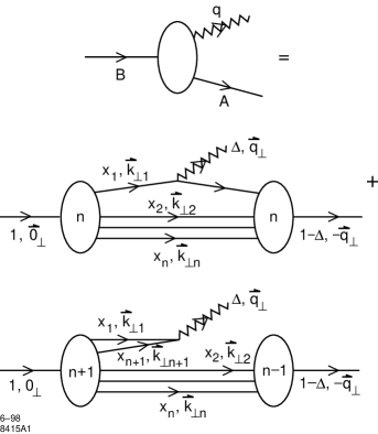
Figure 1: Exact representation of electroweak decays and time-like form factors in the light-cone Fock representation.

The evaluation of the semileptonic decay amplitude $B\to A\ell{\overline{\nu}}$ requires the matrix element of the weak current between hadron states $\left\langle{B|j^{\mu}(0)|A}\right\rangle$. (See Fig. 1.) The interaction current then has simple matrix elements of the free Fock amplitudes, with the provisal that all $x_{i}>0.$ We shall adopt the choice of a Lorentz general frame where the outgoing leptonic current carries $q^{\mu}=\left(q^{+},q_{\perp},q^{-}\right)=\left(\Delta P^{+},q_{\perp},{q^{2}+q^{2}_{\perp}\over\Delta P^{+}}\right)$. In the limit $\Delta\to 0$, the matrix element for the $+$ vector current should coincide with the Drell-Yan formula.

For the $n\to n$ diagonal term ($\Delta n=0$), the final-state hadron wavefunction has arguments $x_{1}-\Delta\over 1-\Delta$, ${\vec{k}}_{\perp 1}-{1-x_{1}\over 1-\Delta}{\vec{q}}_{\perp}$ for the struck quark and $x_{i}\over 1-\Delta$, ${\vec{k}}_{\perp i}+{x_{i}\over 1-\Delta}{\vec{q}}_{\perp}$ for the $n-1$ spectators. We thus have a formula for the diagonal (parton-number-conserving) matrix element of the form:

$${\left\langle{A|J^{\mu}|B}\right\rangle}_{\Delta n=0} = \sum_{n,~{}\lambda}\prod_{i=1}^{n}\int^{1}_{\Delta}dx_{1}\int^{1}_{0}dx_{i(i\neq 1)}\int{d^{2}{\vec{k}}_{\perp i}\over 2(2\pi)^{3}}~{}\delta\left(1-\sum_{j=1}^{n}x_{j}\right)~{}\delta^{(2)}\left(\sum_{j=1}^{n}{\vec{k}}_{\perp j}\right)$$ (1)

$$\times\psi^{\dagger}_{A(n)}(x^{\prime}_{i},{\vec{k}}^{\prime}_{\perp i},\lambda_{i})~{}j^{\mu}~{}\psi_{B(n)}(x_{i},{\vec{k}}_{\perp i},\lambda_{i}),$$

where

$$\left\{\begin{array}[]{lll}x^{\prime}_{1}={x_{1}-\Delta\over 1-\Delta}\,,&{\vec{k}}^{\prime}_{\perp 1}={\vec{k}}_{\perp 1}-{1-x_{1}\over 1-\Delta}{\vec{q}}_{\perp}&\mbox{for the struck quark}\\[4.30554pt] x^{\prime}_{i}={x_{i}\over 1-\Delta}\,,&{\vec{k}}^{\prime}_{\perp i}={\vec{k}}_{\perp i}+{x_{i}\over 1-\Delta}{\vec{q}}_{\perp}&\mbox{for the $(n-1)$ spectators.}\end{array}\right.$$ (2)

A sum over all possible helicities $\lambda_{i}$ is understood. If quark masses are neglected the vector and axial currents conserve helicity. We also can check that $\sum_{i}^{n}x^{\prime}_{i}=1$, $\sum_{i}^{n}{\vec{k}}^{\prime}_{\perp i}={\vec{0}}_{\perp}$.

For the $n+1\to n-1$ off-diagonal term ($\Delta n=-2$), let us consider the case where partons $1$ and $n+1$ of the initial wavefunction annihilate into the leptonic current leaving $n-1$ spectators. Then $x_{n+1}=\Delta-x_{1}$, ${\vec{k}}_{\perp n+1}={\vec{q}}_{\perp}-{\vec{k}}_{\perp 1}$. The remaining $n-1$ partons have total momentum $((1-\Delta)P^{+},-{\vec{q}}_{\perp})$. The final wavefunction then has arguments $x^{\prime}_{i}={x_{i}\over(1-\Delta)}$ and ${\vec{k}}^{\prime}_{\perp i}={\vec{k}}_{\perp i}+{x_{i}\over 1-\Delta}{\vec{q}}_{\perp}$. We thus obtain the formula for the off-diagonal matrix element:

$${\left\langle{A|J^{\mu}|B}\right\rangle}_{\Delta n=-2} = \sum_{n~{}\lambda}\int^{\Delta}_{0}dx_{1}\int^{1}_{0}dx_{n+1}\int{d^{2}{\vec{k}}_{\perp 1}\over 2(2\pi)^{3}}\int{d^{2}{\vec{k}}_{\perp n+1}\over 2(2\pi)^{3}}\prod_{i=2}^{n}\int^{1}_{0}dx_{i}\int{d^{2}{\vec{k}}_{\perp i}\over 2(2\pi)^{3}}$$ (3)

$$\times\delta\left(1-\sum_{j=1}^{n+1}x_{j}\right)~{}\delta^{(2)}\left(\sum_{j=1}^{n+1}{\vec{k}}_{\perp j}\right)$$

$$\times\psi^{\dagger}_{A(n-1)}(x^{\prime}_{i},{\vec{k}}^{\prime}_{\perp i},\lambda_{i})~{}j^{\mu}~{}\psi_{B(n+1)}(\{x_{1},x_{i},x_{n+1}=\Delta-x_{1}\},$$

$$\qquad\ \ \{{\vec{k}}_{\perp 1},{\vec{k}}_{\perp i},{\vec{k}}_{\perp n+1}={\vec{q}}_{\perp}-{\vec{k}}_{\perp 1}\},\{\lambda_{1},\lambda_{i},\lambda_{n+1}=-\lambda_{1}\}).$$

Here $i=2,3,\cdots,n$ with

$$x^{\prime}_{i}={x_{i}\over 1-\Delta}\,,\qquad{\vec{k}}^{\prime}_{\perp i}={\vec{k}}_{\perp i}+{x_{i}\over 1-\Delta}{\vec{q}}_{\perp}$$ (4)

label the $n-1$ spectator partons which appear in the final-state hadron wavefunction. We can again check that the arguments of the final-state wavefunction satisfy $\sum_{i=2}^{n}x^{\prime}_{i}=1$, $\sum_{i=2}^{n}{\vec{k}}^{\prime}_{\perp i}={\vec{0}}_{\perp}$.

The free current matrix elements $j^{\mu}$ in the light-cone representation are easily constructed. For example, the vector current of quarks takes the form

$$j^{\mu}={\overline{u}(x^{\prime},k^{\prime}_{\perp},\lambda^{\prime})\gamma^{\mu}u(x,k_{\perp},\lambda)\over{\sqrt{k^{+}}}{\sqrt{k^{+\prime}}}}$$

and

$$j^{+}=2\delta_{\lambda,\lambda^{\prime}}\ .$$

The other light-cone spinor matrix elements of $j^{\mu}$ can be obtained from the tables in ref. [8]. In the case of spin zero partons

$$j^{+}={x+x^{\prime}\over\sqrt{xx^{\prime}}}$$

and

$$j^{-}={k^{-}+k^{\prime-}\over\sqrt{xx^{\prime}}P^{+}}.$$

However, instead of evaluating each $k^{-}$ in the $j^{-}$ current from the on-shell condition $k^{-}k^{+}=m^{2}$, one must instead evaluate the $k^{-}$ of the struck partons from energy conservation $k^{-}=p^{-}_{\rm initial}-p^{-}_{\rm spectator}$. This effect is seen explicitly when one integrates the covariant current over the denominator poles in the $k^{-}$ variable. It can also be understood as due to the implicit inclusion of local instantaneous exchange contributions obtained in light-cone quantization [9, 10]. The mass $m_{\rm spectator}^{2}$ which is needed for the evaluation of $j^{-}$ current in the diagonal case is the mass of the entire spectator system. Thus $m^{2}_{\perp{\rm spectator}}=m^{2}_{\rm spectator}+{\vec{k}}^{2}_{\perp{\rm spectator}}$, where ${\vec{k}}_{\perp{\rm spectator}}=\sum_{j}{\vec{k}}_{\perp j}$ and $m^{2}_{\perp{\rm spectator}}/x_{\rm spectator}=\sum_{j}m^{2}_{j}/x_{j}$, summed over the $j$ spectators. This is an important simplification for phenomenology, since we can change variables to $m_{\rm spectator}^{2}$ and $d^{2}{\vec{k}}_{\perp{\rm spectator}}$ and replace all of the spectators by a spectral integral over the cluster mass $m_{\rm spectator}^{2}$. A specific example is presented in the next section.

3 Example—$\phi^{3}\$Perturbation Theory

As an explicit example and check on the above formalism, we shall consider the electromagnetic vector current matrix element of a neutral composite system composed of two charged scalars where the light-cone wavefunctions are known explicitly from perturbation theory. To construct the model, we consider a 3+1 dimensional system represented by the Lagrangian:

$${\cal{L}} = (\partial_{\mu}\phi_{a}+ie_{a}A_{\mu}\phi_{a})^{\dagger}(\partial^{\mu}\phi_{a}+ie_{a}A^{\mu}\phi_{a})-m_{a}^{2}\phi_{a}^{\dagger}\phi_{a}$$

$$+(\partial_{\mu}\phi_{b}-ie_{b}A_{\mu}\phi_{b})^{\dagger}(\partial^{\mu}\phi_{b}-ie_{b}A^{\mu}\phi_{b})-m_{b}^{2}\phi_{b}^{\dagger}\phi_{b}$$

$$+{1\over 2}\partial_{\mu}\Phi\partial^{\mu}\Phi-{1\over 2}M^{2}\Phi\Phi+g\Phi(\phi_{a}^{\dagger}\phi_{b}+\phi_{b}^{\dagger}\phi_{a}).$$

The composite system wavefunction can be normalized to unity by a choice of the effective coupling $g$.

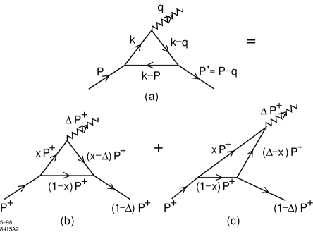
Figure 2: Scalar perturbation theory model for semileptonic decay. (a) Covariant representation. (b), (c) Light-cone time-ordered contributions to the decay amplitude. These contributions can be identified as the convolution of light-cone Fock wavefunctions with $2\to 2$ and $3\to 1$ parton number, respectively.

We can derive the light-cone amplitudes from the covariant amplitude by integrating over the $k^{-}$ variable [11]. The amplitude of the process drawn in Fig. 2 is given as follows from the Feynman rules:

$${\cal M}^{\mu}_{a}$$

$$= ie_{a}g^{2}\int{d^{4}k\over(2\pi)^{4}}\ {(2k-q)^{\mu}\over(k^{2}-m_{a}^{2}+i\epsilon)\ ((k-q)^{2}-m_{a}^{2}+i\epsilon)((k-P)^{2}-m_{b}^{2}+i\epsilon)}$$

$$= ie_{a}g^{2}\int{d^{2}{\vec{k}}_{\perp}\over 2(2\pi)^{4}}\int P^{+}dx\ {1\over P^{+3}x(x-\Delta)(1-x)}$$

$$\times\int dk^{-}{(2k-q)^{\mu}\over\left(k^{-}-{(m_{a}^{2}+{\vec{k}}_{\perp}^{2})-i\epsilon\over xP^{+}}\right)\left((k^{-}-q^{-})-{(m_{a}^{2}+({\vec{k}}_{\perp}-{\vec{q}}_{\perp})^{2}-i\epsilon\over(x-\Delta)P^{+}}\right)\left((k^{-}-P^{-})+{(m_{b}^{2}+{\vec{k}}_{\perp})^{2})-i\epsilon\over(1-x)P^{+}}\right)},$$

where we used $k^{+}=xP^{+}$. When we perform the integration over $k^{-}$, the integral does not vanish only for $0\leq x\leq 1$.

For $\Delta\leq x\leq 1$, which corresponds to Fig. 2(b),

$$({\cal M}^{+}_{a},{\cal M}^{-}_{a},{\vec{\cal M}}_{\perp a})_{(2\to 2)}$$

$$= P^{+}e_{a}g^{2}\int_{\Delta}^{1}dx\int{d^{2}{\vec{k}}_{\perp}\over 2(2\pi)^{3}}$$

$$\times\left((2x-\Delta)\ ,\ {1\over P^{+2}}\left(2\left(M^{2}-{(m_{b}^{2}+{\vec{k}}_{\perp}^{2})\over 1-x}\right)-{(q^{2}+{\vec{q}}_{\perp}^{2})\over\Delta}\right)\ ,\ (2{\vec{k}}_{\perp}-{\vec{q}}_{\perp})\right)$$

$$\times{1\over x(x-\Delta)(1-x)}$$

$$\times{1\over\left(M^{2}-{m_{a}^{2}+{\vec{k}}_{\perp}^{2}\over x}-{m_{b}^{2}+{\vec{k}}_{\perp}^{2}\over 1-x}\right)\left({M^{2}+{\vec{q}}_{\perp}^{2}\over 1-\Delta}-{m_{a}^{2}+({\vec{k}}_{\perp}-{\vec{q}}_{\perp})^{2}\over x-\Delta}-{m_{b}^{2}+{\vec{k}}_{\perp}^{2}\over 1-x}\right)}$$

$$= P^{+}e_{a}g^{2}\int_{\Delta}^{1}dx\int{d^{2}{\vec{k}}_{\perp}\over 2(2\pi)^{3}}$$

$$\times\left((2x-\Delta)\ ,\ {1\over P^{+2}}\left(2\left(M^{2}-{(m_{b}^{2}+{\vec{k}}_{\perp}^{2})\over 1-x}\right)-{(q^{2}+{\vec{q}}_{\perp}^{2})\over\Delta}\right)\ ,\ (2{\vec{k}}_{\perp}-{\vec{q}}_{\perp})\right)$$

$$\times{(1-\Delta)\over x(x-\Delta)(1-x)}$$

$$\times{1\over\left(M^{2}-{m_{a}^{2}+{\vec{k}}_{\perp}^{2}\over x}-{m_{b}^{2}+(-{\vec{k}}_{\perp})^{2}\over 1-x}\right)\left(M^{2}-{m_{a}^{2}+({\vec{k}}_{\perp}+(1-{x-\Delta\over 1-\Delta})(-{\vec{q}}_{\perp}))^{2}\over{x-\Delta\over 1-\Delta}}-{m_{b}^{2}+(-{\vec{k}}_{\perp}-{1-x\over 1-\Delta}(-{\vec{q}}_{\perp}))^{2}\over{1-x\over 1-\Delta}}\right)}$$

$$= P^{+}e_{a}g^{2}\int_{\Delta}^{1}dx\int{d^{2}{\vec{k}}_{\perp}\over 2(2\pi)^{3}}$$

$$\times{1\over{\sqrt{x(x-\Delta)}}}\left((2x-\Delta)\ ,\ {1\over P^{+2}}\left(2\left(M^{2}-{(m_{b}^{2}+{\vec{k}}_{\perp}^{2})\over 1-x}\right)-{(q^{2}+{\vec{q}}_{\perp}^{2})\over\Delta}\right)\ ,\ (2{\vec{k}}_{\perp}-{\vec{q}}_{\perp})\right)$$

$$\times{1\over{\sqrt{x_{a}x_{b}}}}\ {1\over\left(M^{2}-{m_{a}^{2}+{\vec{k}}_{a\perp}^{2}\over x_{a}}\ -{m_{b}^{2}+{\vec{k}}_{b\perp}^{2}\over x_{b}}\right)}\ {1\over{\sqrt{x^{\prime}_{a}x^{\prime}_{b}}}}\ {1\over\left(M^{2}-{m_{a}^{2}+{\vec{k^{\prime}}}_{a\perp}^{2}\over x^{\prime}_{a}}-{m_{b}^{2}+{\vec{k^{\prime}}}_{b\perp}^{2}\over x^{\prime}_{b}}\right)}$$

$$= \int_{\Delta}^{1}dx\int{d^{2}{\vec{k}}_{\perp}\over 2(2\pi)^{3}}$$

$$\qquad\times\psi_{(2)}(x^{\prime}_{a},x^{\prime}_{b},{\vec{k^{\prime}}}_{a\perp},{\vec{k^{\prime}}}_{b\perp};M,m_{a},m_{b})j_{(2\to 2)a}^{\mu}\psi_{(2)}(x_{a},x_{b},{\vec{k}}_{a\perp},{\vec{k}}_{b\perp};M,m_{a},m_{b}),$$

where

$$j_{(2\to 2)a}=e_{a}{P^{+}\over{\sqrt{x(x-\Delta)}}}$$ (8)

$$\qquad\qquad\times\left((2x-\Delta)\ ,\ {1\over P^{+2}}\left(2\left(M^{2}-{(m_{b}^{2}+{\vec{k}}_{\perp}^{2})\over 1-x}\right)-{(q^{2}+{\vec{q}}_{\perp}^{2})\over\Delta}\right)\ ,\ (2{\vec{k}}_{\perp}-{\vec{q}}_{\perp})\right),$$

$$\psi_{(2)}(x_{a},x_{b},{\vec{k}}_{a\perp},{\vec{k}}_{b\perp};M,m_{a},m_{b})=g{1\over{\sqrt{x_{a}x_{b}}}}\ {1\over\left(M^{2}-{m_{a}^{2}+{\vec{k}}_{a\perp}^{2}\over x_{a}}-{m_{b}^{2}+{\vec{k}}_{b\perp}^{2}\over x_{b}}\right)},$$

$$x_{a}=x,\quad x_{b}=1-x,\quad{\vec{k}}_{a\perp}={\vec{k}}_{\perp},\quad{\vec{k}}_{b\perp}=-{\vec{k}}_{\perp},$$

$$x^{\prime}_{a}={x_{a}-\Delta\over 1-\Delta},\quad x^{\prime}_{b}={x_{b}\over 1-\Delta},\quad{\vec{k^{\prime}}}_{a\perp}={\vec{k}}_{a\perp}+(1-x^{\prime}_{a}){\vec{P^{\prime}}}_{\perp},\quad{\vec{k^{\prime}}}_{b\perp}={\vec{k}}_{b\perp}-x^{\prime}_{b}{\vec{P^{\prime}}}_{\perp},$$

$${\vec{P^{\prime}}}_{\perp}=-{\vec{q}}_{\perp}.$$

For $0\leq x\leq\Delta$, which corresponds to Fig. 2(c),

$$({\cal M}^{+}_{a},{\cal M}^{-}_{a},{\vec{\cal M}}_{\perp a})_{(3\to 1)}$$

$$= P^{+}e_{a}g^{2}\int_{0}^{\Delta}dx\int{d^{2}{\vec{k}}_{\perp}\over 2(2\pi)^{3}}$$

$$\times\left((2x-\Delta)\ ,\ {1\over P^{+2}}\left(2{(m_{a}^{2}+{\vec{k}}_{\perp}^{2})\over x}-{(q^{2}+{\vec{q}}_{\perp}^{2})\over\Delta}\right)\ ,\ (2{\vec{k}}_{\perp}-{\vec{q}}_{\perp})\right)$$

$$\times{1\over x(\Delta-x)(1-x)}$$

$$\times{1\over\left(M^{2}-{m_{a}^{2}+{\vec{k}}_{\perp}^{2}\over x}-{m_{b}^{2}+(-{\vec{k}}_{\perp})^{2}\over 1-x}\right)\left(M^{2}-{m_{a}^{2}+{\vec{k}}_{\perp}^{2}\over x}-{m_{a}^{2}+({\vec{q}}_{\perp}-{\vec{k}}_{\perp})^{2}\over\Delta-x}-{M^{2}+{\vec{q}}_{\perp}^{2}\over 1-\Delta}\right)}$$

$$= \int_{0}^{\Delta}dx\int{d^{2}{\vec{k}}_{\perp}\over 2(2\pi)^{3}}\int_{0}^{1}dy\int{d^{2}{\vec{k}}_{y\perp}\over 2(2\pi)^{3}}$$

$$\times\psi_{(1)}\left({y\over 1-\Delta},{\vec{k}}_{y\perp}-{\vec{P^{\prime}}}_{\perp}\right)j_{(3\to 1)a}^{\mu}\psi_{(3)}(x,y,\Delta-x,{\vec{k}}_{\perp},{\vec{k}}_{y\perp},{\vec{q}}_{\perp}-{\vec{k}}_{\perp};M,m_{a},m_{b}),$$

where ${\vec{P^{\prime}}}_{\perp}=-{\vec{q}}_{\perp}$ and

$$j_{(3\to 1)a}^{\mu}=e_{a}{P^{+}\over{\sqrt{x(\Delta-x)}}}$$

$$\qquad\times\left((2x-\Delta)\ ,\ {1\over P^{+2}}\left(2{(m_{a}^{2}+{\vec{k}}_{\perp}^{2})\over x}-{(q^{2}+{\vec{q}}_{\perp}^{2})\over\Delta}\right)\ ,\ (2{\vec{k}}_{\perp}-{\vec{q}}_{\perp})\right),$$ (10)

$$\psi_{(3)}(x,y,\Delta-x,{\vec{k}}_{\perp},{\vec{k}}_{y\perp},{\vec{q}}_{\perp}-{\vec{k}}_{\perp};M,m_{a},m_{b})$$

$$\quad=g^{2}{1\over{\sqrt{x(1-x)^{2}(\Delta-x)y}}}$$

$$\qquad\times{1\over\left(M^{2}-{m_{a}^{2}+{\vec{k}}_{\perp}^{2}\over x}-{m_{b}^{2}+(-{\vec{k}}_{\perp})^{2}\over 1-x}\right)\left(M^{2}-{m_{a}^{2}+{\vec{k}}_{\perp}^{2}\over x}-{m_{a}^{2}+({\vec{q}}_{\perp}-{\vec{k}}_{\perp})^{2}\over\Delta-x}-{M^{2}+{\vec{k}}_{y\perp}^{2}\over y}\right)},$$

$$\psi_{(1)}(y,{\vec{k}}_{y\perp})={{2(2\pi)^{3}\over\sqrt{y}}}\delta(y-1){\delta}^{2}({\vec{k}}_{y\perp}).$$

Then, by combining (3) and (3) the amplitude is given as:

$${\cal M}^{\mu}_{a}$$

$$= \int_{\Delta}^{1}dx\int{d^{2}{\vec{k}}_{\perp}\over 2(2\pi)^{3}}\ \psi_{(2)}(x^{\prime}_{a},x^{\prime}_{b},{\vec{k^{\prime}}}_{a\perp},{\vec{k^{\prime}}}_{b\perp};M,m_{a},m_{b})j_{(2\to 2)a}^{\mu}\psi_{(2)}$$

$$\times(x_{a},x_{b},{\vec{k}}_{a\perp},{\vec{k}}_{b\perp};M,m_{a},m_{b})$$

$$+\int_{0}^{\Delta}dx\int{d^{2}{\vec{k}}_{\perp}\over 2(2\pi)^{3}}\int_{0}^{1}dy\int{d^{2}{\vec{k}}_{y\perp}\over 2(2\pi)^{3}}$$

$$\quad\times\psi_{(1)}\left({y\over 1-\Delta},{\vec{k}}_{y\perp}-{\vec{P^{\prime}}}_{\perp}\right)j_{(3\to 1)a}^{\mu}\psi_{(3)}(x,y,\Delta-x,{\vec{k}}_{\perp},{\vec{k}}_{y\perp},{\vec{q}}_{\perp}-{\vec{k}}_{\perp};M,m_{a},m_{b}).$$

By adding the above amplitude ${\cal M}^{\mu}_{a}$ and that given by exchanging $a$ and $b$ ($e_{a}+e_{b}=0$), we obtain the total amplitude:

$${\cal M}^{\mu}=(2P-q)^{\mu}F(q^{2})$$

$$= \int_{\Delta}^{1}dx\int{d^{2}{\vec{k}}_{\perp}\over 2(2\pi)^{3}}\ \psi_{(2)}(x^{\prime}_{a},x^{\prime}_{b},{\vec{k^{\prime}}}_{a\perp},{\vec{k^{\prime}}}_{b\perp};M,m_{a},m_{b})j_{(2\to 2)a}^{\mu}\psi_{(2)}$$

$$\times(x_{a},x_{b},{\vec{k}}_{a\perp},{\vec{k}}_{b\perp};M,m_{a},m_{b})$$

$$+\int_{0}^{\Delta}dx\int{d^{2}{\vec{k}}_{\perp}\over 2(2\pi)^{3}}\int_{0}^{1}dy\int{d^{2}{\vec{k}}_{y\perp}\over 2(2\pi)^{3}}$$

$$\quad\times\psi_{(1)}\left({y\over 1-\Delta},{\vec{k}}_{y\perp}-{\vec{P^{\prime}}}_{\perp}\right)j_{(3-1)a}^{\mu}\psi_{(3)}(x,y,\Delta-x,{\vec{k}}_{\perp},{\vec{k}}_{y\perp},{\vec{q}}_{\perp}-{\vec{k}}_{\perp};M,m_{a},m_{b})$$

$$\qquad+\ \Bigl{(}a\leftrightarrow b\Bigr{)},$$

where ${\cal M}^{\mu}=(2P-q)^{\mu}F(q^{2})$ follows from $q_{\mu}{\cal M}^{\mu}=0$.

For $q^{2}\rightarrow 0$, ${\vec{q}}_{\perp}\rightarrow{\vec{0}}_{\perp}$ and $\Delta\rightarrow 0$, $+$ component of (3) gives

$$F(0) = e_{a}\int{d^{2}{\vec{k}}_{\perp}\over(2\pi)^{3}}\int_{0}^{1}dx\ |\psi_{(2)}(x,1-x,{\vec{k}}_{\perp},-{\vec{k}}_{\perp};M,m_{a},m_{b})|^{2}$$

$$+e_{b}\int{d^{2}{\vec{k}}_{\perp}\over(2\pi)^{3}}\int_{0}^{1}dx\ |\psi_{(2)}(x,1-x,{\vec{k}}_{\perp},-{\vec{k}}_{\perp};M,m_{b},m_{a})|^{2}\ =\ 0,$$

where $\psi_{(2)}$ is given in (8). Each term can be normalized to unit charge, thus providing wavefunction renormalization in the model. Alternatively we can evaluate the $-$ component of (3) to obtain

$$F(0)$$

$$= e_{a}\int{d^{2}{\vec{k}}_{\perp}\over(2\pi)^{3}}\,{1\over M^{2}}\,\Bigg{(}\int_{0}^{1}dx\ {1\over x}\,\left(M^{2}-{m_{b}^{2}+{\vec{k}}_{\perp}^{2}\over 1-x}\right)|\psi_{(2)}(x,1-x,{\vec{k}}_{\perp},-{\vec{k}}_{\perp};M,m_{a},m_{b})|^{2}$$

$$+{1\over m_{a}^{2}+{\vec{k}}_{\perp}^{2}}g^{2}\Bigg{)}$$

$$+ e_{b}\int{d^{2}{\vec{k}}_{\perp}\over(2\pi)^{3}}\,{1\over M^{2}}\,\Bigg{(}\int_{0}^{1}dx\ {1\over x}\,\left(M^{2}-{m_{a}^{2}+{\vec{k}}_{\perp}^{2}\over 1-x}\right)|\psi_{(2)}(x,1-x,{\vec{k}}_{\perp},-{\vec{k}}_{\perp};M,m_{b},m_{a})|^{2}$$

$$+{1\over m_{b}^{2}+{\vec{k}}_{\perp}^{2}}g^{2}\Bigg{)},$$

where the ${e_{a}\over m_{a}^{2}+{\vec{k}}_{\perp}^{2}}g^{2}$ and ${e_{b}\over m_{b}^{2}+{\vec{k}}_{\perp}^{2}}g^{2}$ terms come from the singular contributions of the $\int_{0}^{\Delta}dx\,\psi_{(1)}\,j_{(3-1)}^{-}\,\psi_{(3)}$ terms in (3) when we take the limit $\Delta\rightarrow 0$. The $\perp$ components of (3) do not give more information since $(2{\vec{P}}-{\vec{q}})_{\perp}\rightarrow{\vec{0}}_{\perp}$ in the left hand side and the integrand of the right hand side is odd about ${\vec{k}}_{\perp}$.

The above analysis provides an explicit realization of the general formulas (1) and (3). In this simple model two transition matrix elements appear: $2\to 2$ and $3\to 1$.

The equality of the formulas for (3) and (3) is a general condition which follows from gauge invariance and consistency of the light-cone formalism. We have verified the equality for the perturbative model by direct evaluation of the integrals.

In the case of general composite systems, the equality of the form factors at zero momentum transfer obtained from the $J^{+}$ and $J^{-}$ currents provides a type of virial theorem for the matrix elements (1) and (3). In general the two determinations of the total charge $F(q^{2}=0)$ must be consistent:

$$F(0) = {1\over 2P^{+}}\,\,\lim_{q^{2},{\vec{q}}_{\perp},\Delta\rightarrow 0}{\left\langle{A|J^{+}|B}\right\rangle}_{\Delta n=0},$$ (15)

$$F(0) = {1\over 2P^{-}}\,\,\lim_{q^{2},{\vec{q}}_{\perp},\Delta\rightarrow 0}\left({\left\langle{A|J^{-}|B}\right\rangle}_{\Delta n=0}+{\left\langle{A|J^{-}|B}\right\rangle}_{\Delta n=-2}\right).$$ (16)

Here $P^{+}P^{-}=M^{2}_{B}.$ Note that the second term of (16) includes the zero mode $\delta(x)$ contributions from the $n+1\to n-1$ off-diagonal matrix element.

4 Conclusions

A most important feature of the light-cone formalism is that all matrix elements of local operators can be written explicitly in terms of simple convolutions of light-cone Fock wavefunctions $\{\psi_{n}(x_{i},k_{\perp i},\lambda_{i})\}$. In the case of exclusive semileptonic $B$-decays, such as $B\rightarrow A\ell\overline{\nu}$, the decay matrix elements require the computation of the diagonal matrix element $n\rightarrow n$ where parton number is conserved and the off-diagonal $n+1\rightarrow n-1$ convolution where the current operator annihilates a $q{\overline{q^{\prime}}}$ pair in the initial $B$ wavefunction. This term is a consequence of the fact that the time-like decay $q^{2}=(p_{\ell}+p_{\overline{\nu}})^{2}>0$ requires a positive light-cone momentum fraction $q^{+}>0$. Conversely for space-like currents, one can choose $q^{+}=0$, as in the Drell-Yan-West representation of the space-like electromagnetic form factors. However, as we have seen from the explicit analysis of the form factor in a perturbation model, the off-diagonal convolution can yield a nonzero $q^{+}/q^{+}$ limiting form as $q^{+}\rightarrow 0$. This extra term appears specifically in the case of “bad” currents such as $J^{-}$ in which the coupling to $q\overline{q}$ fluctuations in the light-cone wavefunctions are favored. In effect, the $q^{+}\rightarrow 0$ limit generates $\delta(x)$ contributions as residues of the $n+1\rightarrow n-1$ contributions. The necessity for this zero mode $\delta(x)$ terms were first noted in the pioneering work of Chang, Root and Yan [9], and Burkardt analyzed it in his studies of higher-twist parton distributions [12]. Here we see that the presence of such terms are a general feature of local operator matrix elements when one selects the simplified $q^{+}=0$ frame.

We have also seen that the proper treatment of the $J^{-}$ current implies new consistency conditions which must be obeyed by the light-cone wavefunctions. For example, current conservation for the form factors of spin zero hadrons requires

$$(2p-q)^{\mu}F(q^{2})=\left\langle{p-q\,|\,J^{\mu}(0)\,|\,p}\right\rangle$$ (17)

and thus

$$\left\langle{p-q\,|\,J^{+}\,|\,p}\right\rangle=\frac{(2p-q)^{+}}{(2p-q)^{-}}\ \left\langle{p-q\,|\,J^{-}\,|\,p}\right\rangle\ .$$ (18)

We have explicitly verified this new type of virial theorem in a simple scalar composite model in section 3.

The off-diagonal $n+1\rightarrow n-1$ contributions provide a new perspective on the physics of $B$-decays. A semileptonic decay involves not only matrix element where a quark changes flavor, but also a contribution where the leptonic pair is created from the annihilation of a $q{\overline{q^{\prime}}}$ pair within the Fock states of the initial $B$ wavefunction. The semileptonic decay thus can occur from the annihilation of a nonvalence quark-antiquark pair in the initial hadron. This feature will carry over to exclusive hadronic $B$-decays, such as $B^{0}\rightarrow\pi^{-}D^{+}$. In this case the pion can be produced from the coalescence of a $d\overline{u}$ pair emerging from the initial higher particle number Fock wavefunction of the $B$. The $D$ meson is then formed from the remaining quarks after the internal exchange of a $W$ boson.

We have emphasized the remarkable advantage of the light-cone formalism that all matrix elements of local operators can be written down exactly in terms of simple convolutions of light-cone Fock wavefunctions. The light-cone wavefunctions depend only on the hadron itself; they are process-independent. The formalism is relativistic and frame-independent—the incident four-vectors can be chosen in any frame. Note that the matrix element of a current in the covariant Bethe-Salpeter formalism requires the construction of the current from insertions into an infinite number of irreducible kernels. The Bethe-Salpeter formalism becomes even more intractable for bound-states of more than two particles.

In principle, a precise evaluation of the hadronic matrix elements needed for $B$-decays and other exclusive electroweak decay amplitudes requires knowledge of all of the light-cone Fock wavefunctions of the initial and final state hadrons. In the case of some model gauge theories such as QCD [13] or collinear QCD [4] in one-space and one-time dimensions, the complete evaluation of the light-cone wavefunction is possible for each baryon or meson bound-state using the discretized light-cone quantization method. It would be interesting to use such solutions as a model for physical $B$-decays.

The evaluation of the light-cone Fock wavefunctions in QCD(3+1) is not at present computationally feasible because of the large number of degrees of freedom within the hadron wavefunctions. Nevertheless, the existence of an exact formalism provides a basis for systematic approximations and a control over neglected terms. For example, one can analyze exclusive semileptonic $B$-decays which involve a heavy internal momentum transfer using a perturbative QCD formalism patterned after the analysis of form factors at large momentum transfer [8]. The hard-scattering analysis proceeds by writing each hadronic wavefunction as a sum of soft and hard contributions

$$\psi_{n}=\psi^{{\rm soft}}_{n}({\cal M}^{2}_{n}<\Lambda^{2})+\psi^{{\rm hard}}_{n}({\cal M}^{2}_{n}>\Lambda^{2}),$$ (19)

where

$${\cal M}^{2}_{n}=\sum^{n}_{i=1}\left(\frac{k^{2}_{\perp}+m^{2}}{x}\right)^{2}_{i}$$ (20)

is the invariant mass of the partons in the $n$-particle Fock state and $\Lambda$ is the separation scale. The high internal momentum contributions to the wavefunction $\psi^{{\rm hard}}_{n}$ can be calculated systematically from QCD perturbation theory from the interaction of the gluon exchange kernel. The contributions from high momentum transfer exchange to the $B$-decay amplitude can then be written as a convolution of a hard scattering quark-gluon scattering amplitude $T_{H}$ with the distribution amplitudes $\phi(x_{i},\Lambda)$, the valence wavefunctions obtained by integrating the constituent momenta up to the separation scale ${\cal M}_{n}<\Lambda<Q$. This is the basis for the perturbative hard scattering analyses of Refs. [7, 14, 15, 16]. In our exact analysis, one can identify the hard PQCD contribution as well as the soft contribution from the convolution of the light-cone wavefunctions. Furthermore, the hard scattering contribution can be systematically improved. For example, off-shell effects can be retained in the evaluation of $T_{H}$ by utilizing the exact light-cone energy denominators. This effect will be analyzed in a separate paper.

Acknowledgements

We wish to thank Chueng-Ryong Ji, Yong-Yeon Keum, Bum-Hoon Lee, and Adam Szczepaniak for helpful discussions. This work was supported in part by the Basic Science Research Institute Program, Ministry of Education, Project No. BSRI-97-2414, and in part by Non-Directed-Research-Fund, Korea Research Foundation 1997.

References

• [1] S.D. Drell and T.M. Yan, Phys. Rev. Lett. 24, 181 (1970).
• [2] S.J. Brodsky and S.D. Drell, Phys. Rev. D22, 2236 (1980).
• [3] G.B. West, Phys. Rev. Lett. 24 1206 (1970).
• [4] F. Antonuccio and S. Dally, Phys. Lett. B348, 55 (1995); Phys. Lett. B376, 154 (1996); Nucl. Phys. B461, 275 (1996).
• [5] H.C. Pauli and S.J. Brodsky, Phys. Rev. D32, 1993 (1985); Phys. Rev. D32, 2001 (1985).
• [6] S.J. Brodsky, H.C. Pauli and S.S. Pinsky, hep-ph/9705477 (1997) (to be published in Physics Reports).
• [7] A. Szczepaniak, E. M.. Henley, and S. J. Brodsky, Phys. Lett .B243 287 (1990).
• [8] G.P. Lepage and S.J. Brodsky, Phys. Rev. D22, 2157 (1980); Phys. Lett. B87, 359 (1979); Phys. Rev. Lett. 43, 545, 1625(E) (1979).
• [9] S.J. Chang, R.G. Root and T.M. Yan, Phys. Rev. D7, 1133 (1973).
• [10] S. J. Brodsky, R. Roskies, and R. Suaya, Phys. Rev D8 4574 (1973).
• [11] M.G. Schmidt, Phys. Rev. D9, 408 (1974).
• [12] M. Burkardt, Nucl. Phys. A504, 762 (1989); Nucl. Phys. B373, 613 (1992); Phys. Rev. D52, 3841 (1995).
• [13] K. Hornbostel, S. J. Brodsky, and H. C. Pauli, Phys. Rev. D41 3814 (1990).
• [14] A. Szczepaniak, Phys. Rev. D54 1167 (1996).
• [15] P. Ball, hep-ph/9802394 (1998); hep-ph/9803501 (1998).
• [16] P. Ball and V.M. Braun, hep-ph/9805422 (1998).