UNIFIED PICTURE OF DIS AND DIFFRACTIVE DIS

The QCD dipole picture allows to build an unified theoretical description -based on BFKL dynamics- of the total and diffractive nucleon structure functions. We use a four parameter fit to describe the 1994 H1 proton structure function $F_{2}$ data in the low $x$, moderate $Q^{2}$ range. Without any additional parameter, the gluon density and the longitudinal structure functions are predicted. The diffractive dissociation processes are discussed within the same framework, and a new 6 parameter fit of the 1994 H1 data is performed which leads to a comprehensive description of $F_{2}^{D(3)}$.

1 Introduction

Considering the phenomenological discussion on the proton structure functions measured by deep-inelastic scattering of electrons and positrons at HERA, it is striking to realize that the proposed models, on one side for the total quark structure function $\!{}^{{\bf?}}$ $F_{2}\left(x,Q^{2}\right)$ and on the other side for its diffractive component $\!{}^{{\bf?}}$ $F_{2}^{D\left(3\right)}\left(x,M^{2},Q^{2}\right)$ are in general distinct.

However, the quest for an unifying picture of total and diffractive structure functions based on a QCD framework is a challenge. The interest of using the QCD dipole approach $\!{}^{{\bf?}}$ for deep-inelastic structure functions is to deal with an unified approach based on the BFKL resummation properties of perturbative QCD $\!{}^{{\bf?}}$.

2 BFKL dynamics and the QCD dipole model

To obtain the proton structure function $F_{2}$, we use the $k_{T}$ factorisation theorem $\!{}^{{\bf?}}$, valid for QCD at high energy (small $x$), in order to factorise the $(\gamma~{}g(k)\rightarrow q~{}\bar{q})$ cross section and the unintegrated gluon distribution of a proton containing the physics of the BFKL pomeron $\!{}^{{\bf?}}$. The detailed calculations can be found in $\!{}^{{\bf?}}$.

We finally obtain:

$$F_{2}\equiv F_{T}+F_{L}={\cal N}a^{1/2}e^{(\alpha_{P}-1)\ln\frac{c}{x}}\frac{Q}{Q_{0}}e^{-\frac{a}{2}\ln^{2}\frac{Q}{Q_{0}}}$$ (1)

where $\alpha_{P}-1=\frac{4\bar{\alpha}N_{C}\ln 2}{\pi}$, and $a=\left(\frac{\bar{\alpha}N_{c}}{\pi}7\zeta(3)\ln\frac{c}{x}\right)^{-1}$. The free parameters for the fit of the H1 data are ${\cal N}$, $\alpha_{P}$, $Q_{0}$, and $c$. Finally, we get $R$, and $F_{G}/F_{2}$, which are independent of the overall normalisation ${\cal N}$ $\!{}^{{\bf?}}$ and represent parameter free predictions of the model once the $F_{2}$ fit is performed.

In order to test the accuracy of the $F_{2}$ parametrisation obtained in formula (1), a fit using the recently published data from the H1 experiment $\!{}^{{\bf?}}$ has been performed $\!{}^{{\bf?}}$. We have only used the points with $Q^{2}\leq 150GeV^{2}$ to remain in the domain of validity of the QCD dipole model. The result of the fit is given in Figure 1. The $\chi^{2}$ is 88.7 for 130 points, and the values of the parameters are $Q_{0}=0.522GeV$, ${\cal N}=0.059,$ and $c=1.750,$ while $\alpha_{P}=0.282$. Commenting on the parameters, the effective coupling constant extracted from $\alpha_{P}$ is $\alpha=0.11$, close to $\alpha(M_{Z})$ used in the H1 QCD fit. It is a small value for the fixed value of the coupling constant required by the BFKL framework. The running of the coupling constant is not taken into account in the present scheme. This could explain the rather low value of the effective $\Delta_{P}$ which is expected to be decreased by the next leading corrections. The value of $Q_{0}$ corresponds to a tranverse size of 0.4 fm which is in the correct range for a proton non-perturbative characteristic scale.

One obtains also a parameter-free prediction for $F_{L}$ $\!{}^{{\bf?}}$ which is in agreement with the (indirect) experimental determination for $F_{L}$ $\!{}^{{\bf?}}$, but somewhat lower than the center values. Thus, it would be interesting to obtain a more precise measurement of $F_{L}$ to test the different predictions on the $Q^{2}$-evolution as already mentionned in Ref. $\!{}^{{\bf?}}$.

Figure 1: Results of the 4-parameter fit of the H1 proton structure function (the fit has been performed using the points with $Q^{2}\leq 150GeV^{2}$). We note a discrepancy at high $x$, high $Q^{2}$ due, in particular, to the absence of the valence contribution not considered in the present model.

3 Diffractive structure functions

The success of the dipole model applied to the proton structure function motivates its extension to the investigations to other inclusive processes, in particular to diffractive dissociation. We can distinguish two different components:
- the “elastic” term which represents the elastic scattering of the onium on the target proton;
- the “inelastic” term which represents the sum of all dipole-dipole interactions (it is dominant at large masses of the excited system).
Let us describe in more details each of the two components. The “inelastic” term dominates at low $\beta$, where $\beta=x/x_{P}$, $x_{P}$ is the proton momentum fraction carried by the colourless exchanged object $\!{}^{{\bf?}}$. This component, integrated over $t$, the momentum transfer, is factorisable in a part depending only on $x_{p}$ (flux factor) and a factor depending only on $\beta$ and $Q^{2}$ (“pomeron” structure function) $\!{}^{{\bf?}}$.

$$F_{2}^{D(3)}(Q^{2},x_{p},\beta)=\Phi(x_{p})F_{P}(Q^{2},\beta)$$ (2)

where $a$ is defined in the first chapter, which gives the following formula for the inelastic component after a saddle point approximation:

$$F_{T,L}^{D(3),inel.}\simeq\frac{1}{x_{P}}\frac{Q}{Q_{0}}a^{3}(x_{P})\;x_{P}^{-2\Delta_{P}}\sqrt{a(\beta)}\beta^{-\Delta_{P}}e^{-\frac{a(\beta)}{2}\log^{2}\frac{Q}{4Q_{0}}}$$ (3)

The important point to notice is that $a(x_{P})$ is proportional of $ln(1/x_{P})$. The effective exponent (the slope of $lnF_{2}^{D}$ in $lnx_{P}$) is found to be dependant on $x_{P}$ because of the term in $ln^{3}(x_{P})$ coming from $a$, and is sizeably smaller than the BFKL exponent. This is why we can describe an apparently softer behaviour with the BFKL equation, which predicts a harder behaviour (the formal exponent in $x_{P}$ is close to 0.35). This is due to the fact that the effective exponent is smaller than the formal one.

For the elastic component, one considers

$$F_{T}^{D(3),el.}\simeq\frac{1}{x_{P}}a^{3}(x_{P})\log^{3}\frac{Q}{2Q_{0}\sqrt{\beta}}\;x_{P}^{-2\Delta_{P}}\;e^{-a(x_{P})\log^{2}\frac{Q}{2Q_{0}\sqrt{\beta}}}$$ (4)

$$\times\beta(1\!-\!\beta)\;\left[{~{}_{2}F_{1}}\left(-\frac{1}{2},\frac{3}{2};2;1-\beta\right)\right]^{2}$$ (5)

and adds ${F_{L}^{D(3),qel.}}$ where $F_{L}$ is obtained from the previous formula by changing ${~{}_{2}F_{1}}\left(-\frac{1}{2},\frac{3}{2};2;1-\beta\right)$ to ${~{}_{2}F_{1}}\left(-\frac{1}{2},\frac{3}{2};1;1-\beta\right)$. The elastic component behaves quite differently $\!{}^{{\bf?}}$ from the inelastic one. First it dominates at $\beta\sim 1$. It is also factorisable like the inelastic component, but with a different flux factor, which means that the sum of the two components will not be factorisable. This means that in this model, factorisation breaking is coming partially from the fact that we sum up two factorisable components with different flux factors. The $\beta$ dependence is quite small at large $\beta$, due to the interplay between the longitudinal and transverse components. The sum remains almost independent of $\beta$, whereas the ratio $R=F_{L}/F_{T}$ is strongly $\beta$ dependent. Once more, a $R$ measurement in diffractive processes will be an interesting way to distinguish the different models, as the dipole model predicts specific $\beta$ and $Q^{2}$ behaviours for $F_{L}$ and $F_{T}$.

We can then compare the H1 data to the following prediction:

$$F_{2}^{D(3)}=F_{2}^{D(3),inel}+F_{2}^{D(3),qel}+F_{2}^{D(3),Reggeon}$$ (6)

where $F_{2}^{D(3),Reggeon}$ represents a secondary trajectory and is taken as in Reference $\!{}^{{\bf?}}$. The free parameters used in the fit are $\alpha_{P}(0)$, $\alpha_{R}(0)$, respectively the exponents for the QCD pomeron and the secondary reggeon, the normalisations in front of the elastic, inelastic and the reggeon terms, and the $Q_{0}$ parameter. The $\chi^{2}$ value obtained is quite good (305.5 for 220 degrees of freedom with statistical error only, 243 for statistical and systematical errors added in quadrature). The values of the parameters are the following: $\alpha_{P}(0)=1.37$, $\alpha_{R}(0)=0.53$ (which is a coventional value for the secondaries), $Q_{0}=0.43$ GeV. The values of $\alpha_{P}(0)$, and $Q_{0}$ are different from those obtained with the $F_{2}$ fit because we used so far approximate formulas to describe diffraction, and because the NLO corrections can behave differently for total and diffractive DIS. The results are given in Figure 2.

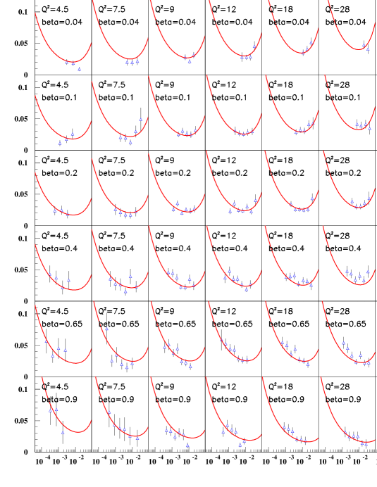
Figure 2: Result of the $F_{2}^{D(3)}fit$ (cf text)                                    

References

References

- [1] H1 coll., Nucl.Phys. B470 (1996) 3
- [2] H1 coll., Z.Phys. C76 (1997) 613
- [3] V.S.Fadin, E.A.Kuraev, L.N.Lipatov Phys. Lett. B60 (1975) 50; I.I.Balitsky and L.N.Lipatov, Sov.J.Nucl.Phys. 28 (1978) 822, V.S. Fadin, L.N.Lipatov, DESY preprint 98-033, G.Camici, M.Ciafaloni, Phys.Lett. B386 (1996) 341, Nucl.Phys. B496 (1997) 305
- [4] A.H.Mueller and B.Patel, Nucl. Phys. B425 (1994) 471., A.H.Mueller, Nucl. Phys. B437 (1995) 107., A.H.Mueller, Nucl. Phys. B415 (1994) 373; N.N.Nikolaev and B.G.Zakharov, Zeit. für. Phys. C49 (1991) 607.
- [5] S.Catani, M.Ciafaloni and Hautmann, Phys. Lett. B242 (1990) 97; Nucl. Phys. B366 (1991) 135; J.C.Collins and R.K.Ellis, Nucl. Phys. B360 (1991) 3; S.Catani and Hautmann, Phys. Lett. B315 (1993) 157; Nucl. Phys. B427 (1994) 475
- [6] H.Navelet, R.Peschanski, Ch.Royon, and S.Wallon, Phys.Lett., B385, (1996) 357, H.Navelet, R.Peschanski, Ch.Royon, Phys.Lett., B366, (1996) 329.
- [7] H1 Coll., Phys.Lett. B393 (1997) 452.
- [8] A.Bialas, R.Peschanski, Phys. Lett. B378 (1996) 302, A.Bialas, Acta Phys.Pol. B27 (1996) no. 6, A.Bialas, R.Peschanski, Phys.Lett. B387 (1996) 405
- [9] A.Bialas, R.Peschanski, Phys.Rev.D, to appear