Torsion action and its possible observables

A.S. Belyaev ${}^{\mbox{a,b,}}$,    I.L. Shapiro ${}^{\mbox{c,d,}}$

${}^{\mbox{a}}$ Instituto de Física Teórica, Universidade Estadual Paulista,
Rua Pamplona 145, 01405-900 - São Paolo, S.P., Brazil

${}^{\mbox{b}}$ Skobeltsyn Institute of Nuclear Physics, Moscow State University,
119 899, Moscow, Russian Federation

${}^{\mbox{c}}\,\,$ Departamento de Física – Instituto Ciencias Exatas, Universidade Federal de Juiz de Fora,
36036-330, Juiz de Fora - MG - Brazil

${}^{\mbox{d}}\,\,$ Tomsk State Pedagogical University, 634041, Tomsk, Russia

The methods of effective field theory are used to explore the theoretical and phenomenological aspects of the torsion field. Spinor action coupled to electromagnetic field and torsion possesses an additional softly broken gauge symmetry. This symmetry enables one to derive the unique form of the torsion action compatible with unitarity and renormalizability. It turns out that the antisymmetric torsion field is equivalent to an massive axial vector field. The introduction of scalars leads to serious problems which are revealed after the calculation of the leading two-loop divergences. Thus the phenomenological aspects of torsion may be studied only for the fermion-torsion systems. In this part of the paper we obtain an upper bounds for the torsion parameters using present experimental data on forward-backward Z-pole asymmetries, data on the experimental limits on four-fermion contact interaction (LEP, HERA, SLAC, SLD, CCFR) and also TEVATRON limits on the cross section of new gauge boson, which could be produced as a resonance at high energy $p\bar{p}$ collisions. The present experimental data enable one to put the limits on torsion parameters for the various range of the torsion mass. We emphasize that for the torsion mass of the order of the Planck mass no any independent theory for torsion is possible, and one must directly use string theory.

Introduction

Despite the impressive success of the Standard Model (SM) there are many reasons to suspect that it doesn’t cover nor all of the existing fields neither all the interactions. The main reason is that the SM unifies strong, weak and electromagnetic interactions while the quantization of gravity remains beyond its scope. It is commonly accepted that the consistent quantum gravity does not exist and that, instead of quantizing gravity itself one has to start with the fundamental theory of different nature which should produce gravity as a low-energy effective theory. The theory of string is a nice example of such a theory: it is consistent as a quantum theory and it induces the gravitational interaction in the low-energy limit (see, for example, [1]). However, along with a metric, the string theory also predicts other constituents of gravity: in particular those are: a scalar field – dilaton and antisymmetric tensor field of the third rank which is usually associated with torsion. The studies of gravity with torsion have a long history (see, for example, [3]) but now the investigation of the possible effects and manifestations of torsion becomes more actual since this can be a possible way to understand the low-energy effects of string physics.

The main theoretical advantage of gravity with torsion is that it links the spin of the matter fields with the space-time geometry. This feature was in a heart of the most of the works about the possible effects of torsion. The classical and quantum theory of fields and particles in an external gravitational field with torsion has been studied in a papers [2, 4, 5, 3, 6, 7, 9, 10, 11, 12, 13, 14, 15] (the reader is referred to these publications and to the review [8] for further references and also to the book [16] for the introduction to quantum field theory in an external gravitational field with torsion). The quantum field theory in an external torsion field predicts many physical effects which we are not going to review here. It is important for us that the renormalizability of quantum theory in an external torsion field requires the nonminimal interaction of an external torsion with a spin-$\frac{1}{2}$ field and also with a scalar field which doesn’t interact with torsion in a minimal way [9]. Thus the interaction of torsion with the spinor field is characterized by the special coupling constant similar to the electron charge. Until now we do not have any positive data about the value of this parameter or about the order of magnitude that the external torsion may have. Moreover without the full theory including the dynamical equations for the torsion itself one can not understand how the external torsion field can be generated in the laboratory. In this situation one promising possibility is to look for an external torsion field which can exist in our part of the Universe. Despite the existing upper bounds for such a field are quite rigid [14] it can be taken responsible [13] for the recently observed anisotropy of the polarization of light coming from some cosmic objects [17].

Independent on the development of the classical and quantum field theory in an external torsion field it is important to establish the form of the action for the torsion itself and to study the possible experimental effects of dynamical torsion. There are, indeed, several known possibilities to approach this problem. In the famous work of Kibble [18] the action of gravity with torsion has been derived as an action of the compensating fields for the general coordinate transformation. Unfortunately this action doesn’t lead to consistent quantum theory since the last is nor unitary neither renormalizable, despite it contains higher derivatives. In the papers [19, 20] many versions of the action of gravity with torsion had been constructed using the condition of unitarity. All those actions are of the second order in curvature and are similar to the Lovelace action which includes the Gauss-Bonnet topological term. Unfortunately those actions are very constrained and the corresponding theory has the renormalizability properties even worst than the action of Kibble.

The problem of renormalizability is casted in another form if we consider it in the content of effective field theory [22, 23]. In the framework of this approach one has to start with the action which includes all possible terms satisfying the symmetries of the theory. Usually such an action contains higher derivatives at least in a vertices. However as far as one is interested in the lower energy effects, those high derivative vertices are suppressed by the huge massive parameter which should be introduced for this purpose. Then those vertices and their renormalization is not visible and effectively at low energies one meets renormalizable and unitary theory. The gauge invariance of all the divergences is guaranteed by the corresponding theorems [24] and thus this scheme may be applied to the gauge theories including even gravity [25]. Within this approach it is important that the lower-derivative counterterms have the same form as a terms included into the action. This condition, together with the symmetries and the requirement of unitarity, may help to construct the effective field theories for the new interactions which are not yet observed, but anticipated from the development of the fundamental theories like string.

If one starts to formulate the dynamical theory for torsion in this framework, the sequence of steps is quite definite. First one has to establish the field content of the dynamical torsion theory and the form of interactions between torsion and other fields. Then it is necessary to take into account the symmetries of this interactions and formulate the action in such a way that the resulting theory is unitary and renormalizable as an effective field theory. Indeed there is no guarantee that all these requirements are consistent with each other, but the inconsistency may only indicate that some symmetries are lost or that the consistent theory with the given particle content is impossible.

In this paper we follow the above scheme and construct the action of torsion coupled to spinor fields which satisfies all the conditions required for the effective quantum theory. Contrary to the other authors [27] we take antisymmetric torsion field to be parametrized by the massive vector field rather than the scalar field because the theory of scalar torsion fails to pass the test of invariant renormalizability. Then we incorporate the Higgs scalar and discuss the violation of consistency which occurs due to the higher loop contributions. After discussion of this problem and its possible solutions we present a phenomenological consideration of the possible effects of the dynamical torsion coupled to the fermions of the SM and derive upper bounds for the torsion parameters from:
1) precisely measured forward-backward Z pole asymmetries at LEP;
2) modern limits on the contact interactions coming from various low and high energy experiments;
3) TEVATRON data on search of the new vector bosons in di-jet channel.

The paper is organized in the following way. In section 2 a brief review of the background notions for the gravity with torsion is given and the form of interaction between torsion and other fields is found. In section 3 the new specific gauge symmetry of the massless part of the spinor action coupled to torsion is outlined. Using this symmetry as a guide we consider the renormalization of the spinor-torsion system and discuss the effective field theory approach to the torsion phenomenology. It will be shown that the new gauge symmetry requires the torsion field to be (equivalent to) massive pseudovector. The explicit calculation of the one-loop divergences confirms this result. Section 4 is devoted to introducing the scalar field and to related difficulties. In section 5 the renormalization group equations for the torsion parameters are explored. We consider the running of the torsion-spinor couplings and the torsion mass and present some arguments that if the values of various spinor-torsion couplings are equal at the Planck scale, then those values are not very different at the lower energies as well. Bearing this in mind we simply put these parameter to be equal for all quarks and leptons and pass to the phenomenological part of the paper. In section 6 we discuss the possible physical observables from which an upper bounds on the torsion mass and fermion-torsion coupling can be derived. In section 7 we analyze the limits on torsion parameters coming from the LEP Z-pole forward-backward lepton and quark asymmetries. Section 8 contains the discussion of a “heavy” torsion for which the torsion phenomenology can be successfully described by the axial-axial contact interactions. Section 9 contains the limits on the torsion parameters from TEVATRON using bounds on the cross section for di-jet events with high invariant mass. In the final section 10 we present our conclusions.

2. Background notions of the gravity with torsion

Let us review the background notions for the gravity with torsion and quantum theory of matter fields in the external torsion field. All the notations correspond to [16] where one can also find a more pedagogical introduction into the subject.

Consider the space - time with independent metric and torsion. The affine connection $\tilde{\Gamma}^{\alpha}_{\;\beta\gamma}$ is nonsymmetric, and the torsion tensor $T^{\alpha}_{\;\beta\gamma}$ is defined as

$${\tilde{\Gamma}}^{\alpha}_{\;\beta\gamma}-{\tilde{\Gamma}}^{\alpha}_{\;\gamma\beta}=T^{\alpha}_{\;\beta\gamma}$$ (1)

The covariant derivative $\tilde{\nabla}_{\mu}$ is based on the nonsymmetric connection $\tilde{\Gamma}^{\alpha}_{\;\beta\gamma}$.  From the metricity condition $\,\tilde{\nabla}_{\mu}g_{\alpha\beta}=0\,$ the solution for the connection can be easily found in the form

$$\tilde{\Gamma}^{\alpha}_{\;\beta\gamma}={\Gamma}^{\alpha}_{\;\beta\gamma}+K^{\alpha}_{\;\beta\gamma}$$ (2)

where ${\Gamma}^{\alpha}_{\;\beta\gamma}$ is usual symmetric Christoffel symbol and $\,\,K^{\alpha}_{\;\beta\gamma}=\frac{1}{2}\,(\,T^{\alpha}_{\;\;\beta\gamma}-T^{\;\alpha}_{\beta\;\gamma}-T^{\;\alpha}_{\gamma\;\beta}\,)\,\,$ is the contorsion tensor. It proves useful to divide the torsion field into three irreducible components:

i)     The vector (trace) $\,\,T_{\beta}=T^{\alpha}_{\;\beta\alpha}$;

ii)    The axial vector (pseudotrace) $\;\,S^{\nu}=\varepsilon^{\alpha\beta\mu\nu}\,T_{\alpha\beta\mu}\;$

iii)   The tensor $\;\,\,q^{\alpha}_{\;\beta\gamma}\;,\;\;\;\;{\rm where}\;\;\;\;\;q^{\alpha}_{\;\beta\alpha}=0\;\;\;\;\;{\rm and}\;\;\;\;\varepsilon^{\alpha\beta\mu\nu}q_{\alpha\beta\mu}=0$.

In general case the torsion field can be presented in the form

$$T_{\alpha\beta\mu}=\frac{1}{3}\,\left(\,T_{\beta}\,g_{\alpha\mu}-T_{\mu}\,g_{\alpha\beta}\,\right)-\frac{1}{6}\,\varepsilon_{\alpha\beta\mu\nu}\,S^{\nu}+q_{\alpha\beta\mu}$$ (3)

One can consider the Dirac spinor $\psi$ in an external gravitational field with torsion using both minimal and nonminimal schemes. The conventional minimal way of introducing the interaction with external fields is to substitute the partial derivatives $\partial_{\mu}$ of spinors by the covariant ${\tilde{\nabla}}_{\mu}$ ones. The covariant derivatives of the spinor field $\psi$ are defined as

$$\tilde{\nabla}_{\mu}\psi=\partial_{\mu}\psi+\frac{i}{2}\,{\tilde{w}}_{\mu}^{\;ab}\,\sigma_{ab}\,\psi\,,\,\,\,\,\,\,\,\,\,\,\,\,\,\,\,\,\,\,\,\,\,\,\,\tilde{\nabla}_{\mu}\bar{\psi}=\partial_{\mu}\bar{\psi}-\frac{i}{2}\,{\tilde{w}}_{\mu}^{\;ab}\,\bar{\psi}\,\sigma_{ab}$$ (4)

where $\tilde{w}_{\mu}^{\;ab}$ are the components of the spinor connection, $\,\sigma_{ab}=\frac{i}{2}(\gamma_{a}\gamma_{b}-\gamma_{b}\gamma_{a})\,,\,$ and we are using the standard representation for the Dirac matrices. The $\,\gamma$-matrices in curved space-time are defined as $\gamma^{\mu}=e_{a}^{\mu}\gamma^{a}$ where $e_{a}^{\mu}$ are the components of the verbein. Indeed $\,\tilde{\nabla}_{\mu}\gamma^{\beta}=0\,$. It is easy to find the explicit expression for spinor connection which agrees with (2).

$$\tilde{w}_{\mu}^{\;ab}=\frac{1}{4}\,(\,e_{\nu}^{b}\,\partial_{\mu}e^{\nu a}-e_{\nu}^{a}\,\partial_{\mu}e^{\nu b}\,)+{\tilde{\Gamma}}^{\alpha}_{\;\nu\mu}\,(e^{\nu a}e_{\alpha}^{b}-e^{\nu b}e_{\alpha}^{a})$$ (5)

Substituting the covariant derivatives (4), (5) into the Hermitian action of the Dirac field

$$S=\frac{i}{2}\,\int d^{4}x\sqrt{-g}\,\left\{\,\bar{\psi}\gamma^{\mu}{\tilde{\nabla}}_{\mu}\psi-{\tilde{\nabla}}_{\mu}\bar{\psi}\,\gamma^{\mu}\psi+2im\,\bar{\psi}\psi\,\right\}$$ (6)

after some algebra we arrive at the following “minimal” action

$$S=\int d^{4}x\sqrt{-g}\,\left\{\,i\bar{\psi}\,\gamma^{\mu}\,(\partial_{\mu}+\frac{i}{8}\,\gamma_{5}\,S_{\mu}\,)\psi\,+\,m\bar{\psi}\psi\,\right\}$$ (7)

Below we will be interested only in the torsion effects and therefore it is reasonable to restrict ourselves by the special case of the flat metric. So we put $g_{\mu\nu}=\eta_{\mu\nu}$ but keep $T^{\alpha}_{\;\beta\gamma}$ arbitrary. One can see that minimally the spinor field interacts only with the pseudovector $S_{\mu}$ part of the torsion tensor. The nonminimal interaction may be a bit more complicated. Using the considerations based on dimensional reasons one can introduce generic nonminimal coupling of the form

$$S=\int d^{4}x\,\left\{\,i\bar{\psi}\gamma^{\mu}\left(\partial_{\mu}+i\eta\gamma_{5}S_{\mu}-i{\hat{\eta}}T_{\mu}\right)\psi\,+\,m\bar{\psi}\psi\,\right\}$$ (8)

Despite the general nonminimal action (8) contains two dimensionless nonminimal parameters $\,\eta,{\hat{\eta}}\,$ we shall use only one of them and put $\,{\hat{\eta}}=0\,$. There are several reasons to do so. As we have already seen the minimal interaction includes only $\eta$ term. In the quantum theory of matter fields on an external torsion background one meets, therefore, $\,\eta\,$ as an essential parameter of the interaction while $\,{\hat{\eta}}=0\,$ is not essential. In other words, if the $\,{\hat{\eta}}=0\,$-term is not included into the classical action, the theory doesn’t lose renormalizability while fixing $\,\eta=\frac{1}{8}\,$ such that interaction is minimal leads to some difficulties [9, 16]. On the other hand, the $\eta$-term looks very similar to the electromagnetic interactions. If we introduce the interaction with the electromagnetic field then the $\eta$-term can be revoked by simple redefinition of the variables and constants. And, as a last reason we can remind that in the string-induced action, which depends on the completely antisymmetric torsion, only the pseudovector part $\,S_{\mu}\,$ is present, and thus one can always set $\,T_{\alpha\beta\mu}=-\frac{1}{6}\,\epsilon_{\alpha\beta\mu\nu}\,S^{\nu}\,.\,$ Below we always use the pseudovector $S_{\mu}$ to parametrize the completely antisymmetric torsion tensor.

With the scalar field $\,\varphi\,$ torsion may interact only nonminimally, because $\,{\tilde{\nabla}}\varphi=\partial\varphi\,$. The action of free scalar field including the nonminimal interaction with antisymmetric torsion has the form

$$S_{sc}=\int d^{4}x\,\left\{\,\frac{1}{2}\,g^{\mu\nu}\,\partial_{\mu}\varphi\,\partial_{\nu}\varphi+\frac{1}{2}\,m^{2}\,\varphi^{2}+\frac{1}{2}\,\xi\,S_{\mu}S^{\mu}\,\varphi^{2}\,\right\}$$ (9)

where $\,\xi\,$ is a new nonminimal parameter. If the quantum theory contains scalar and spinor fields linked by the Yukawa interaction $\,h\varphi{\bar{\psi}}\psi\,$, then the nonminimal parameter $\xi$ is necessary for the renormalizability. For the quantum field theory in the external torsion field the renormalization of the parameters $\,\eta,\xi\,$ possesses some universality. In particular, the $\beta$-function for the nonminimal parameter $\eta$ always has the form

$$\beta_{\eta}=\frac{C}{(4\pi)^{2}}\,h^{2}\,\eta\,,$$ (10)

where the value of the parameter $C$ depends on the model but it is always positive [10]. In section 5 we shall see how the renormalization group equation for $\eta$ modifies in case of the propagating torsion field.

We accept that the gauge vector field do not interact with torsion at all, because such an interaction, generally, contradicts to the gauge invariance. This can be easily seen from the relation

$${\tilde{\nabla}}_{\mu}A_{\nu}-{\tilde{\nabla}}_{\nu}A_{\mu}={\partial}_{\mu}A_{\nu}-{\partial}_{\nu}A_{\mu}+K^{\lambda}_{\;\;\mu\nu}\,A_{\lambda}.$$ (11)

The nonminimal interaction with abelian vector field may be indeed implemented in the form of the surface term

$$S_{n-m,vec}\,=\,i\,\alpha\,\int d^{4}x\,\epsilon^{\alpha\beta\gamma\sigma}\,F_{\alpha\beta}\,S_{\gamma\sigma}.$$ (12)

Other nonminimal terms [16] are also possible for the general torsion but they are relevant only for the nonzero $T_{\mu}$ and $q_{\alpha\beta\gamma}$ of the torsion tensor [10] and thus we are not interested in them here.

3. Effective approach in the spinor-torsion systems

Our aim it to formulate the effective quantum theory of torsion such that it would be compatible with the requirements of renormalizability and unitarity. Let us first consider this problem for the system without scalar fields. As it was already noticed the renormalizability of the gauge model in an external torsion field requires the nonminimal interaction of the spinor fields with torsion [9]. It will prove reasonable to introduce such an interaction in the theory with the propagating torsion too. Thus we start from the action of the Dirac spinor nonminimally coupled to the electromagnetic and torsion fields

$$S_{1/2}=i\,\int d^{4}x\,{\bar{\psi}}\,\left[\,\gamma^{\alpha}\,\left({\partial}_{\alpha}-ieA_{\alpha}+i\,\eta\,\gamma_{5}\,S_{\alpha}\,\right)-im\,\right]\,\psi$$ (13)

and first establish its symmetries. The new interaction with torsion doesn’t spoil the invariance of the above action under usual gauge transformation:

$$\psi^{\prime}=\psi\,e^{\alpha(x)},\,\,\,\,\,\,\,\,\,\,\,\,\,\,{\bar{\psi}}^{\prime}={\bar{\psi}}\,e^{-\alpha(x)},\,\,\,\,\,\,\,\,\,\,\,\,\,\,A_{\mu}^{\prime}=A_{\mu}-{e}^{-1}\,\partial_{\mu}\alpha(x)$$ (14)

It turns out, however, that there is one more symmetry. The massless part of the action (13) is invariant under the transformation in which the pseudotrace of torsion plays the role of the gauge field

$$\psi^{\prime}=\psi\,e^{\gamma_{5}\beta(x)},\,\,\,\,\,\,\,\,\,\,\,\,\,\,{\bar{\psi}}^{\prime}={\bar{\psi}}\,e^{\gamma_{5}\beta(x)},\,\,\,\,\,\,\,\,\,\,\,\,\,\,S_{\mu}^{\prime}=S_{\mu}-{\eta}^{-1}\,\partial_{\mu}\beta(x)$$ (15)

Thus in the massless sector of the theory one faces generalized gauge symmetry depending on scalar $\alpha(x)$ and pseudoscalar $\beta(x)$ parameters of transformation. It is very important that the massive term is not invariant under the transformation (15), and hence this symmetry is softly broken at classical level. The new symmetry (15) requires $S_{\mu}$ to be massive field and fixes the action of torsion with accuracy to the values of the nonminimal parameter $\eta$, mass of the torsion $M_{ts}$ and possible higher derivative terms. The mass of the torsion is necessary because the softly broken symmetry (15) doesn’t forbid the appearance of the massive counterterms (contrary to the situation for the abelian gauge field). We shall give some more arguments in favor of massive torsion in section 5 after discussion of the renormalization group equations. One more inconsistency related with the massless torsion comes from the calculation of the anomalous magnetic moment of the electron, which has been performed recently [28]. Contrary to the abelian vector field, massless axial field leads to the IR divergency.

In the framework of effective field theory the contributions from the loops of a very massive fields are suppressed by the factors of $\,\mu^{2}/M^{2}$ where $M$ is the mass of the field and $\mu$ the typical energy of the process [30]. If we take the torsion mass $M_{ts}$ to be of the Planck order then both classical and quantum effects of torsion will be negligible at the energies available at the modern experimental facilities. The hypothesis of torsion propagating at energies lower than the Planck one supposes that $M_{ts}$ is essentially smaller than the Planck mass. Then we have two options: take torsion to be massless or consider the mass of torsion as a free parameter which should be defined on an experimental basis. As far as torsion is taken as a dynamical field, one has to incorporate it into the SM along with other vector fields. Let us discuss the form of the torsion action, which leads to the consistent quantum theory. The higher derivative terms are supposed to be included into the action, but they are not seen at low energies and thus have no importance. Thus we restrict the torsion action by the second derivative and zero-derivative terms. The general action including these terms has the following form:

$$S_{tor}=\int d^{4}\,\left\{\,-a\,S_{\mu\nu}S^{\mu\nu}+b\,(\partial_{\mu}S^{\mu})^{2}+M_{ts}^{2}\,S_{\mu}S^{\mu}\,\right\}$$ (16)

where $\,S_{\mu\nu}=\partial_{\mu}S_{\nu}-\partial_{\mu}S_{\nu}\,$ and $a,b$ are some positive parameters. The action (16) contains both transversal vector mode and the longitudinal mode which is in fact equivalent to the scalar (see, for example, discussion in [27]) In particular, in the $a=0$ case only the scalar mode, and for $b=0$ only the vector mode propagate. It is well known [31] (see also [27] for the discussion of the theory (16)) that in the unitary theory of the vector field both longitudinal and transversal modes can not propagate, and therefore, in order to have consistent theory of torsion one has to choose one of the parameters $a,b\,$ to be zero.

In fact the only correct choice is $b=0$. To see this one has to reveal that the symmetry (15), which is spoiled by the massive terms only, is always preserved in the renormalization of the dimensionless couplings constants of the theory. In other words, the divergences and corresponding local counterterms, which produce the dimensionless renormalization constants, do not depend on the dimensional parameters such as the masses of the fields. This structure of renormalization is essentially the same as for the Yang-Mills theories with spontaneous symmetry breaking [32, 33]. The symmetry (15) holds for the massless part of the action (13) and therefore on the dimensional grounds one has to expect that the gauge invariant counterterm $\,\,\int S_{\mu\nu}^{2}\,\,$ appears if we take the loop corrections into account.

We want emphasize that in the framework of effective field theory the level of approximation for taking into account the massive fields is qualitatively the same for the tree level and for the lower loop effects. Since the propagating torsion is considered and the kinetic term in (16) is taken into account, one has to formulate the theory as renormalizable. Neglecting the high energy effects while the low energy amplitudes are considered may mean that we disregard some higher derivative terms. However the violation of the renormalizability in that sectors of the theory which are taken into account is impossible. For instance, if we start from the purely scalar longitudinal torsion (as the authors of [27] did) then the transversal term $\,\int S_{\mu\nu}^{2}\,$ will arise with the divergent coefficient and this will indeed violate both the finiteness of the effective action and the unitarity of the $S$-matrix. All this is true even in the case that only the tree-level effects are evaluated, if only such consideration is regarded as an approximation to any reasonable quantum theory.

Thus the kinetic term of the torsion action is given by the Eq. (16) with $b=0$. As concerns the massive term it is not forbidden by the symmetry (15), because the last is softly broken. Therefore apriory there are no reasons to suppose that $M_{ts}=0$. Indeed it is interesting to see whether the kinetic counterterm with $b=0$ and the massive counterterm really appear if we take into account the fermion loops. To investigate this let us calculate the one-loop divergences in the theory (13) . The divergent part of the one-loop effective action is given by the expression

$$\Gamma_{div}[A,S]=-\,\mbox{Tr}\,\ln{\hat{H}}\mid_{\,div}\,;\,\,\,\,\,\,\,\,\,\,\,\,\,\,\,\,\,{\hat{H}}=i\gamma^{\alpha}\,\left({\partial}_{\alpha}-ieA_{\alpha}+i\eta\gamma_{5}\,S_{\alpha}\,\right)-im$$ (17)

In order to calculate this functional determinant one has to perform the transformation

$$\,\mbox{Tr}\,\ln{\hat{H}}=\,\mbox{Tr}\,\ln{\hat{H}}\cdot\left(i\gamma^{\nu}\partial_{\nu}\right)-\,\mbox{Tr}\,\ln\left(i\gamma^{\nu}\partial_{\nu}\right)=\,\mbox{Tr}\,\ln\left(-{\hat{1}}{\Box}-2{\hat{h}}^{\nu}\partial_{\nu}\right)-\,\mbox{Tr}\,\ln\left(i\gamma^{\nu}\partial_{\nu}\right)$$ (18)

with

$${\hat{h}}^{\nu}=\frac{i}{2}\,\left(\,-\,e\,A_{\mu}\,\gamma^{\mu}\gamma^{\nu}\,-\,\eta\,S_{\mu}\,\gamma^{\mu}\gamma_{5}\gamma^{\nu}+m\gamma^{\nu}\,\right)$$

The second term in the right-hand side of Eq. (18) is a constant which doesn’t depend on $S_{\mu}$ or $A_{\mu}$, while the first term can be easily evaluated using the standard Schwinger-deWitt technique (one can see [16] for the introduction and references). After some algebra we arrive at the following counterterm:

$$\Delta S[A_{\mu},S_{\alpha}]=\frac{\mu^{n-4}}{\varepsilon}\int d^{\mu}x\,\left\{\frac{2e^{2}}{3}F_{\mu\nu}F^{\mu\nu}+\frac{2\eta^{2}}{3}S_{\mu\nu}S^{\mu\nu}-\frac{ie\eta}{3}\epsilon^{\alpha\beta\mu\nu}S_{\mu\nu}F_{\alpha\beta}+8m^{2}\eta^{2}S^{\mu}S_{\mu}\right\}$$ (19)

where $\,\varepsilon=(4\pi)^{2}\,(n-4)\,$ is the parameter of the dimensional regularization. Here we disregarded all surface terms except the $\epsilon^{\alpha\beta\mu\nu}\,S_{\mu\nu}F_{\alpha\beta}$ one, because it can, in principle, lead to quantum anomaly. It would be interesting to explore this possibility but since the phenomenological consideration below is mainly restricted by the tree-level effects this term is beyond the scope of our present interest. The form of the counterterms (19) is in perfect agreement with the above analysis based on the symmetry transformation (15). Namely, the one-loop divergences contain $S_{\mu\nu}^{2}$ and the massive term while the $\,\left(\partial_{\nu}S^{\nu}\right)^{2}$ term is absent.

Thus the correct form of the torsion action which can be coupled to the spinor field (13) and lead to the unitary and renormalizable theory is

$$S_{tor}=\int d^{4}\,\left\{\,-\frac{1}{4}\,S_{\mu\nu}S^{\mu\nu}+M_{ts}^{2}\,S_{\mu}S^{\mu}\,\right\}\,.$$ (20)

In the last expression we put the conventional coefficient $\,-1/4$ in front of the kinetic term. With respect to the renormalization this means that we (in a direct analogy with QED) can remove the kinetic counterterm by the renormalization of the field $S_{\mu}$ and then renormalize the parameter $\eta$ in the action (13) such that the combination $\eta S_{\mu}$ is the same for the bare and renormalized quantities. Instead one can include $1/\eta^{2}$ into the kinetic term of (20), that should lead to the direct renormalization of this parameter while the interaction of torsion with spinor has minimal form (7) and $S_{\mu}$ is not renormalized. Therefore in the case of propagating torsion the difference between minimal and nonminimal types of interactions is only the question of notations on both classical and quantum levels.

4. Introducing scalar field

Despite the Higgs scalar is not detected experimentally, it is considered as an important constituent of the SM. The introduction of the scalar field is necessary for the spontaneous symmetry breaking and for the Higgs mechanism which makes the gauge bosons massive and enables one to avoid the infrared divergences in gauge theories. As far as we are going to incorporate torsion into the SM it is important to extend our consideration introducing scalar field and Yukawa interactions. Doing this we shall follow the same line as in the previous section and try first to construct the renormalizable theory. Hence the first thing to do is to analyze the structure of the possible divergences. The divergent diagrams in the theory with a dynamical torsion include, in particular, all such diagrams with external lines of torsion and internal lines of other fields. Those grafs are indeed the same one meets in the quantum field theory on an external torsion background. Therefore one has to include into the action all the terms which were necessary for the renormalizability when torsion was purely external field. All such terms are well-known from [9, 10]. Besides the nonminimal interaction with spinors one has to introduce the nonminimal interaction between scalar field and torsion as in (9) and also the terms which played the role of the action of vacuum (see chapter 4 of [16] where the one-loop counterterms for scalar field are also presented) in the form

$$S_{tor}=\int d^{4}\,\left\{\,-\frac{1}{4}\,S_{\mu\nu}S^{\mu\nu}+M_{ts}^{2}\,S_{\mu}S^{\mu}-\frac{1}{24}\,\zeta\left(S_{\mu}S^{\mu}\right)^{2}\,\right\}+{\rm surface\,terms}\,.$$ (21)

Here $\,\zeta\,$ is new arbitrary parameter, and coefficient $\frac{1}{24}$ stands for the sake of convenience only. And so, if one introduces torsion into the whole SM including the scalar field, the total action includes the following new terms: action of torsion (21) with the self-interacting term, and a nonminimal interactions between torsion and spinors (13) and scalars (9). It is easy to see that such a theory suffers from a serious difficulty.

The root of the problem is that the Yukawa interaction term $\,h\varphi{\bar{\psi}}\psi$ is not invariant under the transformation (15). Unlike the spinor mass the Yukawa constant $h$ is massless, and therefore this noninvariance may affect the renormalization in the massless sector of the theory. In particular, the noninvariance of the Yukawa interaction causes the necessity of the nonminimal scalar-torsion interaction in (9) which, in turn, requires an introduction of the self-interaction term in (21). Those terms do not pose any problem at the one-loop order but already in the second loop one meets two dangerous diagrams presented in Fig. 1

Figure 1: The wavy line is torsion propagator and dashed line – scalar propagator

Those diagrams are divergent and they can lead to the appearance of the $\,\left(\partial_{\mu}S^{\mu}\right)^{2}\,$-type counterterm. No any symmetry is seen which forbids these divergences. Let us consider two diagrams presented on Fig.1 in more details. Using the actions of the scalar field coupled to torsion (9) and the torsion self-interaction (21), we arrive at the following Feynman rules:

i) Scalar propagator: $\,\,\,\,\,\,\,\,\,\,\,\,\,\,\,G(k)=\frac{i}{k^{2}+M^{2}}\,\,{\rm where}\,\,\,M^{2}=2M_{ts}^{2}$,

ii) Torsion propagator: $\,\,\,\,\,\,\,\,\,\,\,\,D_{\mu}^{\,\nu}(k)=\frac{i}{k^{2}+M^{2}}\,\left(\delta_{\mu}^{\,\nu}+\frac{k_{\mu}k^{\nu}}{M^{2}}\,\right)\,\,,$

iii) Torsion²–scalar² vertex: $\,\,\,\,\,\,\,\,\,\,\,\,V^{\mu\nu}(k,p,q,r)\,=\,-\,2i\xi\,\eta^{\mu\nu}\,\,,$

iv) Vertex of torsion self-interaction: $\,\,\,\,\,\,V^{\mu\nu\alpha\beta}(k,p,q,r)\,=\,\frac{i\zeta}{3}\,g_{(2)}^{\mu\nu\alpha\beta}$

where $g_{(2)}^{\mu\nu\alpha\beta}=g^{\mu\nu}g^{\alpha\beta}+g^{\mu\beta}g^{\alpha\nu}+g^{\mu\alpha}g^{\nu\beta}$ and $k,p,q,r$ denote the outgoing momenta.

The only one thing that we would like to check is the violation of the transversality in the kinetic 2-loop counterterms. We shall present the calculation in some details because it is quite instructive. To analize the loop integrals we have used dimensional regularization and in particular the formulas from [35]. It turns out that it is sufficient to trace the $\frac{1}{\varepsilon^{2}}$-pole, because even this leading divergency requires the longitudinal counterterm. The contribution to the mass-operator of torsion from the second diagram from Fig.1 is given by the following integral

$$\Pi^{(2)}_{\alpha\beta}(q)\,=\,-\,2\,\xi^{2}\,\int\frac{d^{D}k}{(2\pi)^{4}}\frac{d^{D}p}{(2\pi)^{4}}\frac{\,\eta_{\alpha\beta}\,+\,M^{-2}\,(k-q)_{\alpha}\,(k-q)_{\beta}\,}{(p^{2}+M^{2})[(k-q)^{2}+M^{2}][(p+k)^{2}+M^{2}]}$$ (22)

To perform the integration one can expand one of the factors in the above integral in the following way:

$$\frac{1}{(k-q)^{2}+M^{2}}=\frac{1}{k^{2}+M^{2}}\,\left[1+\frac{-2k\cdot q+q^{2}}{k^{2}+M^{2}}\right]^{-1}=\frac{1}{k^{2}+M^{2}}\,\sum_{n=1}^{\infty}(-1)^{n}\,\left(\frac{-2k\cdot q+q^{2}}{k^{2}+M^{2}}\right)^{n}$$ (23)

and substitute this expansion into (22). It is easy to see that the divergences hold in this expansion till the order $n=8$. On the other hand, each order brings some powers of the external momenta $q^{\mu}$. Therefore the divergences of the above integral may be cancelled by adding the counterterms which include high derivatives. To achieve the renormalizability one has to include these high derivative terms into the action (21). However, since we are aiming to construct the effective (low-energy) field theory of torsion, the effects of the higher derivative terms are not seen and their renormalization is not interesting for us. All we need are the second derivative counterterms. Hence, for our purposes the expansion (23) can be cut at $n=2$ rather that at $n=8$ and moreover only $O(q^{2})$ terms should be kept. Then, using also usual symmetry considerations, one arrives at the known (see, for example, [35]) intergal

$$\Pi^{(2)}_{\alpha\beta}(q)=-6\xi^{2}\,q^{2}\,\eta_{\alpha\beta}\,\int\frac{d^{D}k}{(2\pi)^{4}}\frac{d^{D}p}{(2\pi)^{4}}\,\frac{1}{p^{2}+M^{2}}\,\frac{1}{(k^{2}+M^{2})^{2}}\,\frac{1}{(p+k)^{2}+M^{2}}+\,...\,=$$

$$=-\frac{12\,\xi^{2}}{(4\pi)^{4}\,(D-4)^{2}}\,q^{2}\,\eta_{\alpha\beta}\,+\,({\rm lower}\,\,{\rm poles})\,+\,({\rm higher}\,\,{\rm derivative}\,\,{\rm terms}).$$ (24)

Another integral looks a bit more complicated, but its derivation performs in a similar way. The contribution to the mass-operator of torsion from the first diagram from Fig.1 is given by the integral

$$\Pi^{(1)}_{\alpha\lambda}(q)=-\frac{\zeta^{2}}{108}\,g^{(2)\alpha\rho\sigma\beta}\,g^{(2)\lambda\tau\mu\nu}\,\int\frac{d^{4}k}{(2\pi)^{4}}\,\int\frac{d^{4}p}{(2\pi)^{4}}\,\frac{1}{k^{2}+M^{2}}\left(\eta_{\tau\beta}+\frac{k_{\tau}k_{\beta}}{M^{2}}\right)\times$$

$$\times\left(\eta_{\rho\mu}+\frac{(p-q)_{\rho}(p-q)_{\mu}}{M^{2}}\right)\,\frac{1}{p^{2}+M^{2}}\,\left(\eta_{\sigma\nu}+\frac{(p+k)_{\sigma}(p+k)_{\nu}}{M^{2}}\right)\,\frac{1}{(k+q)^{2}+M^{2}}$$ (25)

Now, we perform the same expansion (23) and, disregarding lower poles, finite contributions and higher derivative leading divergences arrive at

$$\Pi^{(1)}_{\alpha\lambda}(q) = -\frac{\zeta^{2}}{108}\,g^{(2)\alpha\rho\sigma\beta}\,g^{(2)\lambda\tau\mu\nu}\,\times$$ (26)

$$\times 3\,q^{2}\,\eta_{\tau\beta}\,\eta_{\rho\mu}\,\eta_{\sigma\nu}\,\int\frac{d^{4}k}{(2\pi)^{4}}\,\int\frac{d^{4}p}{(2\pi)^{4}}\,\frac{1}{k^{2}+M^{2}}\frac{1}{(p^{2}+M^{2})^{2}}\frac{1}{(k+p)^{2}+M^{2}}\,+\,...\,.$$

After a simple algebra this leads to the following leading divergency

$$\Pi^{(1)}_{\alpha\lambda}(q)=-\frac{\zeta^{2}}{(4\pi)^{4}\,(D-4)^{2}}\,q^{2}\,\eta_{\alpha\lambda}+\,...\,.$$ (27)

Thus we see that both diagrams from Fig.1 really give rise to the longitudinal kinetic counterterm and no any simple cancellation of these divergences is seen. On the other hand one can hope to achieve such a cancellation on the basis of some sofisticated symmetry.

To understand the situation better let us compare it with the one that takes place for the usual abelian gauge transformation (14). In this case the symmetry is not violated by the Yukawa coupling, and (in the abelian case) the $\,A^{2}\varphi^{2}\,$ counterterm is impossible because it violates gauge invariance. The same concerns also the self-interacting $A^{4}$ counterterm. The gauge invariance of the theory on quantum level is controlled by the Ward identities. In principle, the noncovariant counterterms can show up, but they can be always removed, even in the non-abelian case, by the renormalization of the gauge parameter and in some special class of (background) gauges they are impossible at all. Generally, the renormalization can be always performed in a covariant way [24].

In case of the transformation (15) if the Yukawa coupling is inserted there are no reasonable gauge identities at all. Therefore in the theory of torsion field coupled to the SM with scalar field there is a conflict between renormalizability and unitarity. The action of the renormalizable theory has to include the $\,\left(\partial_{\mu}S^{\mu}\right)^{2}\,$ term, but this term leads to the problems with the positivity of the energy and, in terms of particles, to the appearance of the massive ghost. This conflict between unitarity and renormalizability reminds the one which is well known – the problem of massive unphysical ghosts in the high derivative gravity [36], where the contributions of the massive ghosts provide renormalizability but breaks the unitarity of the $S$-matrix. The difference is that in our case, unlike higher derivative gravity, the problem appears due to the noninvariance with respect to the transformation (15).

Let us now discuss how this problem may be, in principle, solved. First thought is that if the torsion mass is of the Planck order then the quantum effects of torsion should be described directly in the framework of string theory. No any effective field theory for torsion is possible. In this case the only visible term in the torsion action is the massive one in (21), torsion does not propagate at smaller energies and manifests itself only as a very weak contact interaction. We shall give the discussion of these contact interactions below in section 7, however the phenomenological analysis fails for $M_{ts}$ well below the Planck order.

There may be a hope to impose one more symmetry which is not violated by the Yukawa coupling. It can be, for example, supersymmetry which mixes torsion with some vector fields of the SM and with all massive spinor fields. In this case the $\,\left(\partial_{\mu}S^{\mu}\right)^{2}\,$-type counterterm may be forbidden by this symmetry and the conflict between renormalizability and unitarity would be resolved.

Another option is to consider the modification of SM which is free from the fundamental scalar fields at all. This possible scenario is related with the fact that there is one crucial point of SM which still remains unclear: the pattern of electroweak symmetry breaking which generates masses for the $W$ and $Z$ bosons. Moreover, we still lack the same accuracy tests for the triple and quartic bosonic interactions to further confirm the local gauge invariance of the theory or to indicate the existence of new physics beyond the SM.

The interactions responsible for the electroweak symmetry breaking play an important role in the gauge–boson interactions at the TeV scale since it is an essential ingredient to avoid unitarity violation in the scattering amplitudes of massive vector bosons at energies of the order of 1 TeV [37]. There are two possible forms of electroweak symmetry breaking sector which lead to different solutions to the unitarity problem: there is, either, a scalar particle lighter than 1 TeV, the Higgs boson of the Standard Model (SM), or such particle is absent and the longitudinal components of the $W$ and $Z$ bosons become strongly interacting at the energy scale of 1 TeV. In the latter case, the symmetry breaking occurs due to the nonzero vacuum expectation value of some composite operators, and it is related with some new underlying physics. Then the spontaneous symmetry breaking can be realized through some other object like composite scalar field or maybe through the torsion itself.

In the future sections of the paper we are going to discuss a possible consequences of the torsion action at low energies (as compared to the Planck one) and find some numerical upper bounds for the parameters of this action. Since the interaction with the scalar field leads to serious problems, we shall consider only the interaction between torsion and spinor field, and therefore use (20) as the torsion action. Thus we admit that one of the two last options (or some other) for the resolution of the problem with the scalar field may be successfully realized and that $M_{ts}$ is much less that the Planck mass. So, instead of taking the string-inspired mass $M_{Pl}$ we take $M_{ts}$ to be some free parameter of the theory, as we do with a couplings $\eta$. Indeed the last may be different for various quarks and leptons.

5. Renormalization group and the running of torsion mass and parameters

In this section we shall discuss the renormalization group in the theory with torsion. First we consider the spinor-torsion system with an additional electromagnetic field, but without the controversial scalar. Then the renormalization group equations for the parameters $\,e,\eta,m,M_{ts},\alpha$ (here $\alpha$ is the parameter of the nonminimal term (12)) follow from Eq. (19).

$$(4\pi)^{2}\,\frac{de}{dt}=\frac{2}{3}\,e^{2}\,,\,\,\,\,\,\,\,\,\,\,\,\,\,\,\,\,\,\,\,\,e(0)=e_{0}$$ (28)

$$(4\pi)^{2}\,\frac{d\eta}{dt}=\frac{2}{3}\,\eta^{2}\,,\,\,\,\,\,\,\,\,\,\,\,\,\,\,\,\,\,\,\,\,\eta(0)=\eta_{0}$$ (29)

$$(4\pi)^{2}\,\frac{d\alpha}{dt}=\frac{1}{3}\,e\,\eta\,,\,\,\,\,\,\,\,\,\,\,\,\,\,\,\,\,\,\,\,\,\alpha(0)=\alpha_{0}$$ (30)

$$(4\pi)^{2}\,\frac{dM_{ts}^{2}}{dt}=8\,m^{2}\,\eta^{2}-2\,M_{ts}^{2}\,,\,\,\,\,\,\,\,\,\,\,\,\,\,\,\,\,\,\,\,\,M_{ts}(0)=M_{ts,0}$$ (31)

We remark that the equation (31) demonstrates the inconsistency of the massless or very light torsion. Even if one imposes the normalization condition $M_{ts,0}\approx 0$ at some scale $\mu$, the first term in this equation provides a rapid change of $M_{ts}$ such that it will be essentially nonzero at other scales. Due to the universality of the interaction (13) all quarks and massive leptons should contribute to this equation. Therefore the only way to avoid an unnaturally fast running of $M_{ts}$ is to take its value at least of the order of the heaviest spinor field that is $t$-quark. Hence we have some grounds to take $M_{ts}\geq 100\,$GeV. Of course there can not be any upper bounds for $M_{ts}$ from the equation (31).

The solution of the equations (28) – (30) for the dimensionless parameters is simple. After the simple calculus we get

$$e(t)=e_{0}\,\left(1-\frac{2\,e_{0}^{2}\,t}{3\,(4\pi)^{2}}\right)^{-1}\,,\,\,\,\,\,\,\,\,\,\,\,\,\,\,\,\,\eta(t)=\eta_{0}\,\left(1-\frac{2\,\eta_{0}^{2}\,t}{3\,(4\pi)^{2}}\right)^{-1}\,,$$ (32)

$$\alpha(t)=A\,+\,\frac{3\,e_{0}\,\eta_{0}}{2\,(e_{0}-\eta_{0})}\ln\left(\frac{1-\frac{2\,\eta_{0}^{2}}{3(4\pi)^{2}}\,t}{1-\frac{2\,e_{0}^{2}}{3(4\pi)^{2}}\,t}\right)\,,\,\,\,\,\,\,\,\,\,\,\,\,\,\,\,\,e_{0}\neq\eta_{0}\,\,,\,\,\,\,\,\,\,\,\,\,\,\,\,\,A=const.$$ (33)

The behavior of the effective couplings $\,e(t),\eta(t)\,$ is usual for the nonabelian vector fields, and the running of $\eta$ is universal for all the spinors. The zero-charge problem doesn’t impose real restrictions on $\eta$ because for $\,\eta<1\,$ the singular point of the solution is many orders bigger than $M_{Pl}$.

In order to see how the difference between various spinor fields may arise let us consider the theory with the scalar fields and Yukawa coupling but in the one-loop approximation where the formal problems discussed in the previous section do not show up. At the one-loop level the $\beta$-functions for the different $\eta$’s come from the renormalization of the kinetic term for torsion of the $\,\,{\bar{\psi}}\gamma_{5}\gamma^{\mu}S_{\mu}\psi$-type. The last ones are the same as for the quantum field theory in an external torsion field. Taking into account (10) the full renormalization group equation for $\eta(t)$ is written as

$$(4\pi)^{2}\,\frac{d\eta}{dt}=\frac{2}{3}\,\eta^{2}+C\,h^{2}(t)\,\eta\,,\,\,\,\,\,\,\,\,\,\,\,\,\,\,\,\,\,\,\,\,\eta(0)=\eta_{0}$$ (34)

One can use (34) to evaluate the difference between the running of $\,\eta\,$ for different spinor fields. Let us take, for simplicity, constant $h$. Then the solution of (34) has the form

$$\frac{\eta(t)}{\eta_{0}}=\frac{3Ch}{2}\,\left[\,(\eta_{0}+\frac{3Ch}{2}\,)\cdot exp\left\{-\frac{Cht}{(4\pi)^{2}}\right\}-\eta_{0}\right]^{-1}$$ (35)

If we suppose that the value of $\eta_{0}$ is very small, then the terms containing $\eta_{0}$ in the right-hand side can be abandoned and we arrive at the following approximate solution

$$\frac{\eta(\mu)}{\eta_{0}}=\left[\frac{\mu}{\mu_{0}}\right]^{\frac{Ch}{(4\pi)^{2}}}$$ (36)

Taking the normalization scale $\mu_{0}=100\,$GeV and the high-energy scale $\mu=M_{Pl}=10^{19}$GeV, we find that for the $t$-quark Yukawa constant $h_{t}\approx 0.98$ this ratio is about $10^{0.105\cdot C}$. The value of $C$ depends on the gauge group and representation which we do not know for all the energy ranges between $\mu_{0}$ and $M_{Pl}$. Taking, for instance, the adjoint representation of the $SU$(5) group we meet $C=5$ [16], and therefore the ratio (36) is about $3.4$ for the $t$-quark while it is close to one for the light spinors which have small Yukawa couplings. We note that taking into account the running of $h(t)$ the resulting ratio becomes a bit smaller.

Suppose the spinor fields are generated from some fundamental theory at the Planck scale and originally have universal interaction with torsion, with an equal parameters $\eta$. Then the difference in the values of $\eta$ for various fields should be caused by the running. As we have just seen, in the framework of this (essentially one-loop) model these parameters still have the same order of magnitude at the Fermi scale. Below we consider the processes which involve only one type of the spinor fields, and hence for our purposes it is not so important whether various $\eta$’s have equal value. However this information will be implicitly used when we construct the general limits for the torsion parameters from various known experiments.

6. Phenomenology of torsion

As we have already seen, the spinor-torsion interactions enter the Standard Model as interactions of fermions with new axial vector field $S_{\mu}$. Such an interaction is characterized by the new dimensionless parameter – coupling constant $\eta$. Furthermore the mass of the torsion field $M_{ts}$ is unknown, and its value is of crucial importance for the possible experimental manifestations of the propagating torsion and finally for the existence of torsion at all. In this and consequent sections we consider $\,\eta\,$ and $\,M_{ts}\,$ as an arbitrary parameters and try to limit their values from the known experiments. Indeed we use the renormalization group as an insight concerning the mass of torsion but include the discussion of the ”light” torsion with the mass of the order of 1 GeV for the sake of generality.

Our strategy will be to use known experiments directed to the search of the new interactions. We regard torsion as one of those interactions and obtain the limits for the torsion parameters from the data which already fit with the phenomenological considerations. Therefore in the course of our work we insert torsion into the minimal SM and suppose that the other possible new physics is absent. It is common assumption when one wants to put limits on some particular kind of a new physics. In the following sections we put the limits on the parameters of the torsion action using results of various experiments.

Torsion, being a pseudo-vector particle interacting with fermions might give therefore different physical observables. The main feature of torsion is related with its axial vector type interaction with fermions. This specific type of interaction might lead to the forward-backward asymmetry. The last has been presizely measured at the LEP $e^{+}e^{-}$ collider, so the upper bounds for torsion parameters may be set from those measurements. We will consider two different cases: i) torsion is much more heavy than other particles of SM and    ii) torsion has a mass comparable to that of other particles. In the last case one meets a propagating particle which must be treated on an equal footing with other constituents of the SM. Contrary to that, the very heavy torsion leads to the effective contact four-fermion interactions.

Consider the case of heavy torsion in some more details, starting from the actions (13) and (20). Since the massive term dominates over the covariant kinetic part of the action, the last can be disregarded. Then the total action leads to the algebraic equation of motion for $\,S_{\mu}$. The solution of this equation can be substituted back to $\,S_{1/2}+S_{tor}\,$ and thus produce the contact four-fermion interaction term

$${\cal L}_{int}=-\frac{\eta^{2}}{M_{ts}^{2}}\,({\bar{\psi}}\gamma_{5}\gamma^{\mu}\psi)\,({\bar{\psi}}\gamma_{5}\gamma_{\mu}\psi)$$ (37)

As one can see the only one quantity which appears in this approach is the ratio ${M_{ts}}/{\eta}\,$ and therefore for the very heavy torsion field the phenomenological consequences depend only on single parameter.

Physical observables related with torsion depend on the two parameters $M_{ts}$ and $\eta$. In the course of our study we choose, for the sake of simplicity, all the torsion couplings with fermions to be the same $\eta$. This enables one to put the limits in the two dimensional ($M_{ts}$-$\eta$) parameter space using the present experimental data. We also assume that non-diagonal coupling of the torsion with the fermions of different families is zero in order to avoid flavor changing neutral current problem.

It should be stressed that all numerical and symbolic calculations for establishing limits on torsion parameters have been done using CompHEP software package [39] to which the torsion propagator and vertices were additionally introduced.

7. Limits on the torsion parameters from presize LEP electroweak data

As we mentioned above, the axial-vector type interactions would give rise to the forward-backward asymmetry which have been presizely measured in the $e^{+}e^{-}\rightarrow l^{+}l^{-}(q\bar{q})$ scattering (here $l$ stands for tau,muon or electron) at LEP collider with the center-mass energy equals to the Z-boson mass, in other words near the Z-pole. Due to the resonance production of Z-bosons the statistics is good (several million events) and it allowed to measure electroweak (EW) parameters with high precision.

Any parity violating interactions eventually give rise to the space asymmetryand could be revield in, for example, forward-backward asymmetry measurement. Axial-vector type interactions of torsion with matter fields is this case of interactions. But the source of asymmetry also exists in the SM EW interactions because of the presense of the $\gamma_{\mu}\gamma_{5}$ structure in the interactions of $Z$- and $W$-bosons with fermions. The interactions between $Z$-boson and fermions can be written in general form as:

$$L_{Zff}=-\frac{g}{2\,cos\theta_{W}}\sum_{i}\,{\bar{\psi}}_{i}\,\gamma^{\mu}(g^{i}_{V}-g^{i}_{A}\gamma^{5})\psi\,Z_{\mu}\,,$$ (38)

where, $\theta_{W}$ is Weinberg angle, $g=e/sin\theta_{W}$ ($e$ - positron charge); and the vector and axial couplings are:

$$g_{V}^{i} \equiv t_{3L}(i)-2q_{i}\,sin^{2}\theta_{W},$$ (39)

$$g_{A}^{i} \equiv t_{3L}(i).$$ (40)

Here $t_{3L}$ is the weak isospin of fermion and $i$ has the values $+1/2$ for $u_{i}$ and $\nu_{i}$ while it is $-1/2$ for $d_{i}$ and $e_{i}$. Here $i=1,2,3\,$ is the index of the fermion generation and $q_{i}$ is the charge of the $\psi_{i}$ in units of charge of positron.

The left handed fermion fields $\psi_{i}=$ $\left(\begin{array}[]{c}\nu_{i}\\ e^{-}_{i}\end{array}\right)$ and $\left(\begin{array}[]{c}u_{i}\\ d^{\prime}_{i}\end{array}\right)$ of the i^th fermion family transform as a doublets under SU(2), where ${d^{\prime}}_{i}\equiv\sum_{j}V_{ij}d_{j}$ and $V$ is the Cabibbo-Kobayashi-Maskawa mixing matrix.

The forward-backward asymmetry for $e^{+}e^{-}\rightarrow l^{+}l^{-}$ is defined as

$$A_{FB}\equiv\frac{\sigma_{F}-\sigma_{B}}{\sigma_{F}+\sigma_{B}},$$ (41)

where $\sigma_{F}(\sigma_{B})$ is the cross section for $l^{-}$ to travel forward(backward) with respect to electron direction. Such an asymmetries are measured at LEP 1.

From asymmetries one derives the ratio $g_{V}/g_{A}$ of vector and axial-vector couplings. Presence of torsion would change the forward-backward asymmetry and would, as we show below, brightly reviel itself. In fact, the measured EW parameters are in a good agreement with the theoretical predictions and hence one can establish the limits on the torsion parameters based on the experimental errors. The latest relevant electroweak data are presented in Table 1.

$A{FB}$	$A^{l}_{FB}$	$A^{b}_{FB}$	$A^{c}_{FB}$
data	0.0171(10)	0.0984(24)	0.0741(48)
$g_{V}$	$g_{Ve}$	$g_{V\mu}$	$g_{V\tau}$
data	-0.0367(15)	-0.0374(36)	-0.0367(15)
$g_{A}$	$g_{Ae}$	$g_{A\mu}$	$g_{A\tau}$
data	-0.50123(44)	-0.50087(66)	-0.50102(74)

Table 1: Results of combined LEP EW measurements for forward-backward asymmetry at Z-pole and vector and axial couplings. $A^{l}_{BF}$ – combined data for electron, muon and tau-lepton asymmetries; $A^{b}_{BF}$ and $A^{c}_{BF}$ – asymmetries for b-quark and c-quark respectively.

Hereafter we will use $A^{l}_{BF}$ value for combined lepton asymmetry and in particular for the electron $A^{e}_{BF}$ asymmetry in establishing the limits on the torsion parameters. We have calculated the contribution to the asymmetries from torsion exchange diagrams shown in Fig. 2.

Figure 2: Diagrams with torsion exchange in $e^{+}e^{-}$ collisions contributing to forward-backward lepton and quark asymmetry. TS indicates to the torsion propagators.

From those calculations we have found limits at $95\%$ confidence level (CL) on the $\eta$ coupling for different torsion masses taking into account the error of the experimental measurements. The most precise individual measurement at LEP is from $A^{b}_{FB}$. But it turned out that the most restrictive limit on $\eta$ comes from the electron asymmetry of $e^{-}e^{+}\rightarrow e^{-}e^{+}$ scattering since in this case both ($s$- and $t$-channel) diagrams from the Fig. 2 contribute to $A^{e}_{FB}$. In the case of $e^{-}e^{+}\rightarrow b\bar{b}$ only $s$-channel diagram (the first one on the Fig. 2) does contribute to the $A^{b}_{FB}$ asymmetry. $A^{e}_{FB}$ and $A^{b}_{FB}$ $Z$-pole asymetries for $Z$-bozon exchange diagram and for the diagrams with the torsion exchange, shown in Fig. 2 can be written as follows:

$$A_{FB}^{e(b)}=\frac{(\sigma_{F}-\sigma_{B})^{e(b)}}{(\sigma_{F}+\sigma_{B})^{e(b)}},$$ (42)

where $(\sigma_{F}-\sigma_{B})^{e(b)}$ and $(\sigma_{F}+\sigma_{B})^{e(b)}$ are the following expressions:

$$(\sigma_{F}-\sigma_{B})^{e} = K_{l}\left[\frac{e^{4}{g_{a}^{e}}^{2}{g_{v}^{e}}^{2}M_{Z}^{2}}{2c_{W}^{4}s_{W}^{4}\Gamma_{Z}^{2}}+\frac{e^{2}\eta^{2}M_{TS}}{2c_{W}s_{W}\Gamma_{Z}}[({g_{a}^{e}}^{2}+{g_{v}^{e}}^{2})F_{1}^{FB}-2{g_{v}^{e}}^{2}F_{2}^{FB}]+\eta^{4}F_{3}^{FB}\right]$$ (43)

$$(\sigma_{F}-\sigma_{B})^{b} = K_{q}\left[\frac{e^{4}{g_{a}^{e}}{g_{a}^{b}}{g_{v}^{e}}{g_{v}^{b}}M_{Z}^{2}}{2c_{W}^{4}s_{W}^{4}\Gamma_{Z}^{2}}-\frac{4e^{2}\eta^{2}M_{TS}}{3c_{W}s_{W}\Gamma_{Z}}{g_{v}^{e}}{g_{v}^{b}}F_{2}^{FB}\right]$$ (44)

$$(\sigma_{F}+\sigma_{B})^{e} = K_{l}\left[\frac{e^{4}({g_{a}^{e}}^{2}+{g_{v}^{e}}^{2})^{2}M_{Z}^{2}}{6c_{W}^{4}s_{W}^{4}\Gamma_{Z}^{2}}+\frac{e^{2}\eta^{2}M_{TS}}{2c_{W}s_{W}\Gamma_{Z}}[({g_{a}^{e}}^{2}+{g_{v}^{e}}^{2})F_{1}^{T}-\frac{8}{3}{g_{v}^{e}}^{2}F_{2}^{T}]+\eta^{4}F_{3}^{T}\right]$$ (45)

$$(\sigma_{F}+\sigma_{B})^{b} = K_{q}\left[\frac{e^{4}({g_{a}^{e}}^{2}+{{g_{v}^{e}}^{2}})({g_{a}^{b}}^{2}+{g_{v}^{b}}^{2})M_{Z}^{2}}{6c_{W}^{4}s_{W}^{4}\Gamma_{Z}^{2}}-\frac{4e^{2}\eta^{2}M_{TS}}{3c_{W}s_{W}\Gamma_{Z}}{g_{v}^{e}}{g_{v}^{b}}F_{2}^{T}\right],$$ (46)

Here $s_{W}$ and $c_{W}$ are $sin$ and $cos$ of the Weinberg angle, $\Gamma_{Z}$ – width of $Z$-boson, $K_{l}=1/(16\pi M_{Z}^{2})$,   $K_{q}=3/(16\pi M_{Z}^{2})$,   $F_{1,2,3}^{FB(T)}$ function are written as follows:

$$F_{1}^{FB}=-z-\frac{4(1+z^{2})^{2}y_{1}}{z^{3}},$$

$$F_{2}^{FB}=F_{2}^{T}=\frac{z^{3}}{z^{2}-1},$$

$$F_{3}^{FB}=\frac{4z^{2}(1+2z^{2}+2z^{4})}{(z^{2}+1)(z^{2}+2)}+\frac{2z^{2}}{z^{2}-1}+\frac{8(3+z^{2})}{z^{2}-1}y_{1}$$ (47)

$$F_{1}^{T}=\frac{-z^{2}(2+3z^{2})+2(1+z^{2})^{2}y_{2}}{z^{3}},$$

$$F_{3}^{T}=4(1+z^{2})-\frac{2z^{2}}{1+z^{2}}+\frac{8z^{4}}{3(1-z^{2})^{2}}+\frac{4(2+3z^{2})-8(1+z^{2})y_{2}}{(z^{2}-1)},$$ (48)

where

$$z=\frac{M_{Z}}{M_{TS}}\,,\,\,\,\,\,y_{1}=ln\frac{1+z^{2}}{(1+z^{2}/2)^{2}}\,,\,\,\,\,\,y_{2}=ln(1+z^{2})\,.$$ (49)

When torsion exchange is absent ($\eta=0$), then from the formulaes below one obtains a well known result [38] for tree level SM asymmetries:

$$A^{b(e)}_{FB}=\frac{3{g_{a}^{e}}{g_{a}^{b(e)}}{g_{v}^{e}}{g_{v}^{b(e)}}}{({g_{a}^{e}}^{2}+{g_{v}^{e}}^{2})({g_{a}^{b(e)}}^{2}+{g_{v}^{b(e)}}^{2})}$$ (50)

Electroweak radiative corrections can be absorbed into $g_{a}$ and $g_{v}$ values formulae written above will be valid including loop corrections for redefined $g_{a}$ and $g_{v}$ values. Figure 3a) and b) shows the behavior of the $A^{e}_{FB}$ and $A^{b}_{FB}$ asymmetries respectively versus $\eta$ torsion coupling when torsion mass is fixed to 1 TeV. We use electroweak parameters of $M_{Z}$, $\Gamma_{Z}$, $sin\theta_{W}$, $g_{A(V)}$ from [38]. One can see that $A^{b}_{FB}$ asymmetry depends much weaker on $\eta$ and goes down with increasing of $\eta$ while $A^{e}_{FB}$ is increasing with increasing of $\eta$. For zero $\eta$ the asymmetries are equal to it’s SM predictions (which is slightly different from measured value, see [38] for details). They are not zero because of the presence of the axial-vector coupling in the interactions of $Z$-boson and electron or quark. Deviations of the asymmetry from SM predictions would be indication of the presense of the additional torsion-like type axial-vector interactions. Our analysis shows that $A^{e}_{FB}$ asymmetry is the best observable among others asymmetries to look for torsion.

Figure 3: Forward-backward $\,e^{-}e^{+}\rightarrow e^{-}e^{+}\,$ and $\,e^{-}e^{+}\rightarrow b\bar{b}\,$ asymmetries versus torsion $\,\eta\,$ coupling

Exclusion region for $(\eta,M_{TS})$ plane coming from this asymmetry is shown in Fig. 4(A). Some numbers corresponding to this limit are presented in Table 2.

$M_{ts}$(GeV)	1	10	50	100	200	1000	3000
$\eta$	0.018	0.050	0.18	0.18	0.48	2.6	9.9

Table 2: Points for exclusion curve at 95% CL in ($M_{ts},\eta$) plane from LEP Z-pole $A_{FB}^{e}$ asymmetry. These numbers correspond to the Fig. 4(A).

8. Torsion and 4-fermion contact interactions

The straightforward consequence of the heavy torsion interacting with fermion fields is the effective four-fermion contact interaction of leptons and quarks (37). Four-fermion interaction effectively appears for the torsion with a mass much higher than the energy scale available at present colliders. In this section we are going to set an upper bounds for the single parameter ${M_{ts}}/{\eta}\,$ from (37) using modern data. There are several experiments from which the constraints on the contact four-fermion interactions come:

1)Experiments on polarized electron-nucleus scattering – SLAC e-D scattering experiment[40], Mainz e-Be scattering experiment [41] and bates e-C scattering experiment [42]; 2)Atomic physics parity violations measures [43] electron-quark coupling that are different from those tested at high energy experiment provides alternative constraints on new physics. 3) $e^{+}e^{-}$ experiments - SLD, LEP1, LEP1.5 and LEP2 (see for example [44, 45, 46, 47, 48]); 4)Neutrino-Nucleon DIS experiments – CCFR collaboration obtained model independent constraint on the effective $\nu\nu qq$ coupling [49].

Here we consider a limits on the contact interactions induced by torsion. The contact four-fermion interaction may be described by the Lagrangian [52] of the most general form:

$$L_{\psi^{\prime}\psi^{\prime}\psi\psi}=g^{2}\sum_{i,j=L,R}\sum_{q=u,d}\frac{\epsilon_{ij}}{(\Lambda_{ij}^{\epsilon})^{2}}\,(\bar{\psi}^{\prime}_{i}\gamma_{\mu}\psi^{\prime}_{i})\,(\bar{\psi}_{j}\gamma^{\mu}\psi_{j})$$ (51)

Subscripts i,j refer to different fermion helicities: $\,\psi^{(^{\prime})}_{i}=\psi^{(^{\prime})}_{R,L}=(1\pm\gamma_{5})/2\cdot\psi^{(^{\prime})}\,$; where $\psi^{(^{\prime})}$ could be quark or lepton; $\,\,\Lambda_{ij}\,$ represents the mass scale of the exchanged new particle; coupling strength is fixed by the relation: $\,g^{2}/4\pi=1$, the sign factor $\,\epsilon_{ij}=\pm 1\,$ allows for either constructive or destructive interference with the SM $\gamma$ and $Z$-boson exchange amplitudes. The formula (51) can be successfully used for the study of the torsion-induced contact interactions because it includes an axial-axial current interactions as a particular case.

Recently the global study of the electron-electron-quark-quark($eeqq$) interaction sector of the SM [51] have been done using data from all mentioned experiments. The limits established in this paper are the best in comparison with the previous ones.

The specific distinguishing feature of the contact interactions induced by torsion is that those contact interactions are of axial-axial type. Therefore we used the limits obtained in paper [51] for this kind of interaction. Limits on axial-axial ($AA$) type contact interactions mainly come from OPAL collaboration. It was shown (see for details [45]) that present LEP data are particulary sensitive to $VV$ and $AA$ models which could be distinguished from others types of contact interactions by analysing of scattering angle distributions of outgoing leptons and quarks. The other possibility of study the chiral structure of contact interactions through the polarized lepton and proton beams scattering analysis can be realized at HERA [50].

Axial-axial current may be expressed through $\,LL,RR,LR\,\,{\rm and}\,\,RL\,$ currents in the following way:

$$j_{\mu}^{A}j_{\mu}^{A}=\frac{j_{\mu}^{L}j_{\mu}^{L}+j_{\mu}^{R}j_{\mu}^{R}-j_{\mu}^{L}j_{\mu}^{R}-j_{\mu}^{R}j_{\mu}^{L}}{4}\,.$$ (52)

For the axial-axial $\,eeqq\,$ interactions (51) takes the form (we put $g^{2}=4\pi$) :

$$L_{eeqq}=-\frac{4\pi}{{(\Lambda_{AA}^{\epsilon})^{2}}}(\bar{e}\gamma_{\mu}\gamma_{5}e)(\bar{q}\gamma^{\mu}\gamma_{5}q)$$ (53)

The limit for the contact axial-axial $eeqq$ interactions comes from the global analysis of Ref. [51]:

$$\frac{4\pi}{\Lambda_{AA}^{2}}<0.36\mbox{ TeV}^{-2}$$ (54)

Comparing the parameters of the effective contact four-fermion interactions of general form (53) and contact four fermion interactions induced by torsion (37) we arrive at the following relations:

$$\frac{\eta^{2}}{M_{ts}^{2}}=\frac{4\pi}{{\Lambda_{AA}}^{2}}$$ (55)

From (54) and (55) one gets the following limit on torsion parameters:

$$\frac{\eta}{M_{ts}}<0.6\mbox{ TeV}^{-1}\;\Rightarrow\;M_{ts}>1.7\mbox{ TeV }\cdot\eta$$ (56)

Figure 4: Allowed regions for $M_{ts}$ and $\eta$ coming from LEP $A^{e}_{FB}$ asymmetry at Z-pole (A), global study of electron-quark contact interactions (B), LEP1.5 (C) and TEVETRON data (D). (E) – combined limit. Hatched region is excluded by experiments mentioned above at 95% CL

The limits on $M_{ts}$ and $\eta$ coming from the (56) is shown in Figure 1(B). As we have already mentioned above the restrictions concern only the ratio between the torsion mass and coupling parameter. Some remark about the energy limits taken in this plot is in order. We started exclusion region from $M_{ts}=$ 1 TeV. This choice is related with the fact that the application of effective-contact interactions (37) is valid up to the certain mass of the torsion below which an exact calculation (regarding the field $S_{\mu}$ as dynamical) should be done. The relative data of the two approaches are shown on the Figure 2, where the results for gauge interaction (20) and contact interactions (51) for torsion are compared. As an example we have calculated total cross section for LEP1.5 with $\sqrt{s}=140$ GeV and $\eta$ equal to 0.5. One can clearly see that for torsion heavier than 1 TeV the approximation of the effective contact interaction works almost perfectly, reproducing the result for the exact calculation with 0.1% accuracy. Therefore the scale 1 TeV is appropriate starting point for putting the limit on torsion parameters using the Lagrangian with contact interactions.

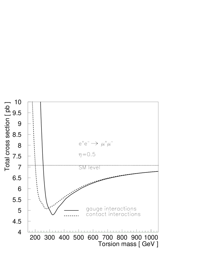
Figure 5: Comparison of the total cross sections of $e^{+}e^{-}\rightarrow\mu^{+}\mu^{-}$ process for gauge and contact interactions

Scenario with light torsion is in general more difficult because here we have two independent parameters and thus are enforced to study the $2$-dimensional restrictions from the experimental data. Indeed there is no rigid border between two cases, as we shall see below.

To consider the limits in the ($M_{ts},\eta$) parameter space for the light torsion we use results of LEP1.5 analysis of paper [45]: the cross section of $e^{+}e^{-}\rightarrow e^{+}e^{-}(\mu^{+}\mu^{-})$ process was measured with accuracy 1-2%. We used this fact to put the limits on torsion mass and coupling: 90% acceptance for electron and 60% for muon channels was assumed, the total cross section for these reaction were calculated and 4% deviation from the Standard Model prediction was taken for establishing the limits. The resulting constraints is shown in Figure 4(C).

9. Limits on the torsion parameters from TEVATRON data

The torsion with the mass in the range of present colliders could be produced in fermion-fermion interactions as a resonance, decaying to fermion pair. The most promising collider for search the signature of such type is TEVATRON. This proton-antiproton 1.8 TeV collider has the highes available center of mass energy up to the moment. So one can naturally expect that the haviest resonance which could be produced in the quark-quark, quark-gluon or gluon-gluon collision would be discovered there.

Search for New Particles Decaying to two-jets has been done recently by D0 and CDF collaborations [53]. The data that we use in our analysis are extracted from the figure presented by the D0 collaboration which established the limit on the production cross section of $Z^{\prime}$ and $W^{\prime}$ bosons. Here we assume also 90% events efficiency (including efficiency of kinematical cuts and trigger efficiency) and calculated the cross section for torsion production at TEVATRON. For simplicity we also assumed that torsion coupling with only one kind of quark (u-quark) is nonzero and calculated the cross section of the reaction $p\bar{p}(u\bar{u})\rightarrow TS\rightarrow u\bar{u}$. Then we applied D0 limit at 95% CL for torsion production cross section and converted into the limit for ($M_{ts},\eta$) plane. This limit is shown in Fig. 4(D). The points for the exclusion curve are given in Table 3.

$M_{ts}$(GeV)	200	300	400	500	600	700	800
$\eta$	0.17	0.18	0.12	0.13	0.17	0.27	0.34

Table 3: Points for exclusion curve in ($M_{ts},\eta$) plane from TEVATRON data( 95% CL). See Fig. 4(D).

One can see that the limits on $\eta$ coming from these analysis are better in comparison with those from the LEP data for some values of $\,\eta\,$ parameter. Combined exclusion plot for  ($M_{ts},\eta$)  plane is presented in Fig. 4(E).

10. Conclusions

Starting from the fermion-torsion coupling we have derived the action of the propagating torsion and implemented it into the abelian sector of the Standard Model. It was shown that the only one action of torsion which leads to consistent effective field theory includes propagating pseudovector massive particle with softly broken (new) gauge symmetry. The renormalization group gives a strong argument against the light torsion, because, due to the universality of torsion-fermion interaction, light torsion means an unnaturally fast running of the torsion mass. Since the scalar fields and Yukawa coupling are inconsistent with propagating torsion, we base the phenomenological part of our work on the fermion sector of the SM only. In this way, we have established some upper bounds on the torsion mass and torsion-fermion coupling constant (which is supposed to be universal) using combined limit for asymmetry of the forward-backward scattering, four-fermion contact interactions and also LEP and TEVATRON data. For heavy torsion the limit is described by relation (56) while for light torsion with the mass below 1 TeV limits coming from LEP and TEVATRON data bound $\eta$ to be less than 0.1-0.02 depending on $M_{ts}$.

Results presented above clearly show, that the best limits for light torsion could be obtained from LEP asymmetry data. In particular for the $M_{ts}<$ 1 GeV the value of $\eta$ is less than 0.02. This gives an essential improvement as compared to our previous report [26] where this kind of observables was not considered. The limits of the same order or may be even better could be obtained from data on the measurement of the anomalous magnetic moment for electron and muon [28]. At the same time the best limits for heavy torsion come from global analysis of contact interactions [51].

In the case of a very heavy mass $\,M_{ts}\sim M_{Pl}\,$ the torsion manifests itself only as an extremely weak contact interaction. The propagation and quantum effects of such a torsion may be described only in the framework of string theory. In other words such a “very heavy” torsion doesn’t exist as an independent field. In this paper we have studied the alternative option.

Acknowledgments

Authors are grateful to M. Asorey, I.L. Buchbinder, J.A. Helayel-Neto, I.B. Khriplovich and T. Kinoshita for stimulating discussions. We are also indebted to M. Kalmykov for sharing with us the results of calculations [28] prior to publication.  I. L. Sh. acknowledges warm hospitality of Departamento de Física, Universidade Federal de Juiz de Fora and partial support by CNPq (Brazil) and by Russian Foundation for Basic Research under the project No.96-02-16017. A. S. B. is grateful to the Instituto de Física Teórica for its kind hospitality and acknowledges support from Fundação de Amparo à Pesquisa do Estado de São Paulo (FAPESP).

References

- [1] M.B. Green, J.H. Schwarz and E. Witten, Superstring Theory (Cambridge University Press, Cambridge, 1987).
- [2] B.K. Datta,Nuovo Cim. 6B (1971) 1; 16.
- [3] F.W. Hehl, Gen. Relat.Grav.4(1973)333;5(1974)491; F.W. Hehl, P. Heide, G.D. Kerlick and J.M. Nester, Rev. Mod. Phys.48 (1976) 3641.
- [4] J. Audretsch, Phys.Rev. 24D (1981) 1470.
- [5] H. Rumpf,Gen. Relat. Grav. 14 (1982) 773.
- [6] Goldthorpe W.H.,Nucl. Phys.170B (1980) 263; Cognola G., Zerbini S.,Phys.Lett.214B (1988) 70; Gusynin V.P.,Phys.Lett.225B (1989) 233; Nieh H.T., Yan M.L.,Ann. Phys.138 (1982)237.
- [7] H. Rumpf, Gen.Rel.Grav. 10 (1979) 509; 525; 647.
- [8] ”On the gauge aspects of gravity”, F. Gronwald, F. W. Hehl, GRQC-9602013, Talk given at International School of Cosmology and Gravitation: 14th Course: Quantum Gravity, Erice, Italy, 11-19 May 1995, gr-qc/9602013
- [9] I.L. Buchbinder and I.L. Shapiro, Phys.Lett. 151B (1985) 263.
- [10] I.L. Buchbinder and I.L. Shapiro, Class. Quantum Grav. 7 (1990) 1197; I.L. Shapiro, Mod.Phys.Lett.9A (1994) 729.
- [11] V.G. Bagrov, I.L. Buchbinder and I.L. Shapiro, Izv. VUZov, Fisica (in Russian, English translation: Sov.J.Phys.) 35,n3 (1992) 5; see also hep-th/9406122.
- [12] R. Hammond, Phys.Lett. 184A (1994) 409; Phys.Rev. 52D (1995) 6918.
- [13] A. Dobado and A. Maroto, Mod.Phys.Lett. A12 (1997) 3003.
- [14] C. Lammerzahl, Phys.Lett. 228A (1997) 223.
- [15] L.H. Ryder and I.L. Shapiro, Phys.Lett.A, to be published.
- [16] I.L. Buchbinder, S.D. Odintsov and I.L. Shapiro, Effective Action in Quantum Gravity. (IOP Publishing – Bristol, 1992).
- [17] B. Nodland and J. Ralston, Phys.Rev.Lett., 78 (1997) 3043.
- [18] T.W. Kibble, J.Math.Phys. 2 (1961) 212
- [19] D.E. Nevill, Phys.Rev. D18 (1978) 3535.
- [20] E. Sezgin and P. van Nieuwenhuizen, Phys.Rev. D21 (1980) 3269.
- [21] Zwiebach B., Phys.Lett. 156B (1985) 315; Deser S. and Redlich A.N., Phys.Lett.176B (1986) 350; Jones D.R.T., Lowrence A.M., Z.Phys. 42C (1989) 153.
- [22] S. Weinberg, The Quantum Theory of Fields: Foundations. (Cambridge Univ. Press, 1995).
- [23] J.F. Donoghue, E. Golowich and B.R. Holstein, Dynamics of the Standard Model (Cambridge University Press, 1992).
- [24] B.L. Voronov, P.M. Lavrov and I.V. Tyutin, Sov.J.Nucl.Phys. 36 (1982) 498; J. Gomis and S. Weinberg, Nucl.Phys. B469 (1996) 473.
- [25] Donoghue J.F., Phys.Rev.Lett. 72 (1994) 2996; Phys.Rev.D50 (1994) 3874.
- [26] A.S. Belyaev and I.L. Shapiro, Phys.Lett. B, to be published.
- [27] S.M. Caroll and G.B. Field, Phys.Rev. 50D (1994) 3867.
- [28] M. Yu. Kalmykov, private communication.
- [29] M. Novello, Phys.Lett. 59A (1976) 105.
- [30] T. Appelquist and J. Corrazone, Phys.Rev. D11 (1975) 2856.
- [31] L.D. Faddeev and A.A. Slavnov, Gauge fields. Introduction to quantum theory. (Benjamin/Cummings, 1980).
- [32] S. Weinberg, Phys.Rev. 118 838.
- [33] B.L. Voronov and I.V. Tyutin, Sov.J.Nucl.Phys. 23 (1976) 664.
- [34] I.L. Buchbinder, S.D. Odintsov and I.L. Shapiro, Phys.Lett. 162B (1985) 92.
- [35] J.A. Helayel-Neto, Il.Nuovo Cim. 81A (1984) 533; J.A. Helayel-Neto, I.G. Koh and H. Nishino, Phys.Lett. 131B (1984) 75.
- [36] K.S. Stelle, Phys.Rev. 16D, 953 (1977).
- [37] B. Lee, C. Quigg and H. Thacker, Phys. Rev. Lett. 38, 883 (1977); Phys. Rev. D16, 1519 (1977); D. Dicus and V. Mathur, Phys. Rev. D7, 3111 (1973).
- [38] The LEP Electroweak Working Group, CERN-PPE/97-154 (1997).
-
[39]
E.E.Boos, M.N.Dubinin, V.A.Ilyin, A.E.Pukhov, V.I.Savrin,
SNUTP-94-116, INP-MSU-94-36/358,
hep-ph/9503280;
P.A.Baikov et al., Proc. of X Workshop on HEP and QFT (QFTHEP-95), ed. by B.Levtchenko, V.Savrin, p.101, hep-ph/9701412. - [40] C.Y. Prescott et al., Phys. Lett. B84, 524 (1979)
- [41] W. Heil et al., Nucl. Phys. B327, 1 (1989)
- [42] WP.A. Souder et al., Phys.Rev.Lett. 65, 694 (1990)
- [43] P.Langasker, M.Luo and A.Mann, Rev.Mod.Phys. 64, 86 (1992)
- [44] LEP Collaborations and SLD Collaboration, “A Combination of Preliminary Electroweak Measurements and Constrains on the Standard Model”, prepared from contributions to the 28th International Conference on High Energy Physics, Warsaw, Poland, CERN-PPE/96-183 (Dec. 1996).
- [45] OPAL Collaboration, G. Alexander et al., B391, 221 (1996).
- [46] L3 Collaboration, Phys. Lett. B370, 195 (1996); CERN-PPE/97-52, L3 preprint 117 (May 1997).
- [47] ALEPH Collaboration, Phys. Lett. B378, 373 (1996).
- [48] P. Langacker and J. Erler, presented at the Ringberg Workshop on the Higgs Puzzle, Ringberg, Germany, 12/96, hep-ph/9703428.
- [49] K.S. McFarland et al. (CCFR), FNAL-Pub-97/001-E, hep-ex/9701010.
- [50] J.M. Virey, CPT-97-P-3542, To be published in the proceedings of 2nd Topical Workshop on Deep Inelastic Scattering off Polarized Targets: Theory Meets Experiment (SPIN 97), Zeuthen, Germany, 1-5 Sep 1997: Working Group on ’Physics with ”Polarized Protons at HERA” ,hep-ph/9710423
- [51] V. Barger, K. Cheung, K. Hagiwara, D. Zeppenfeld; MADPH-97-999, hep-ph/9707412. We are thankful to the authors of this paper for their analysis.
- [52] E.Eichten, K.Lane, and M.Peskin, Phys.Rev.Lett. 50, 811 (1983).
- [53] CDF Collaboration and D0 Collaboration (Tommaso Dorigo for the collaboration), FERMILAB-CONF-97-281-E, 12th Workshop on Hadron Collider Physics (HCP 97), Stony Brook, NY, 5-11 Jun 1997