YUMS 98–10

SNUTP 98–52

DESY 98–77

PM 98–14

IFT/9/98

June 1998

Chargino Pair Production in $e^{+}e^{-}$ Collisions

S.Y. Choi¹, A. Djouadi², H. Dreiner³,

J. Kalinowski⁴ and P.M. Zerwas⁵

¹ Department of Physics, Yonsei University, Seoul 120–749, Korea ² Phys. Math. et Théorique, Université Montpellier II, F–34095 Montpellier, France ³ Rutherford Laboratory, Chilton, Didcot OX11 OQX, U. Kingdom ⁴ Inst. Theor. Physics, Warsaw University, PL–00681 Warsaw, Poland ⁵ DESY, Deutsches Elektronen-Synchrotron, D–22603 Hamburg, Germany

Charginos $\chi_{1}^{\pm}$ are expected to be the lightest observable supersymmetric particles in many supersymmetric models. We present a procedure which will allow to determine the chargino mixing angles and, subsequently, the fundamental SUSY parameters $M_{2},\mu$ and $\tan\beta$ by measurements of the total cross section and the spin correlations in $e^{+}e^{-}$ annihilation to $\chi_{1}^{+}\chi_{1}^{-}$ chargino pairs.

1. Introduction

In supersymmetric theories, the spin–1/2 partners of the $W$ boson and charged Higgs boson, $\tilde{W}^{\pm}$ and $\tilde{H}^{\pm}$, mix to form chargino mass eigenstates $\tilde{\chi}^{\pm}_{1,2}$. The mass eigenvalues $m_{\tilde{\chi}_{1,2}^{\pm}}$ and the mixing angles $\phi_{L},\phi_{R}$ are determined by the elements of the chargino mass matrix in the $(\tilde{W}^{-},\tilde{H}^{-})$ basis [1]

$${\cal M}_{C}=\left(\begin{array}[]{cc}M_{2}&\sqrt{2}m_{W}\cos\beta\\ \sqrt{2}m_{W}\sin\beta&\mu\end{array}\right)$$ (3)

which is built up by the fundamental supersymmetric parameters: the gaugino mass $M_{2}$, the Higgs mass parameter $\mu$, and the ratio $\tan\beta=v_{2}/v_{1}$ of the vacuum expectation values of the two neutral Higgs fields which break the electroweak symmetry. Once charginos will have been discovered, the experimental analysis of their properties, production and decay mechanisms, will therefore reveal the basic structure of the underlying low–energy supersymmetric theory.

Charginos are produced in $e^{+}e^{-}$ collisions, either in diagonal or in mixed pairs [2]. In the present note, we will focus on the diagonal pair production of the lightest chargino $\tilde{\chi}_{1}^{\pm}$ in $e^{+}e^{-}$ collisions,

$$e^{+}e^{-}\ \rightarrow\ \tilde{\chi}^{+}_{1}\ \tilde{\chi}^{-}_{1}$$

The second chargino $\tilde{\chi}_{2}^{\pm}$ is generally expected to be significantly heavier than the first state. At LEP2 [3], and potentially even in the first phase of $e^{+}e^{-}$ linear colliders (see e.g. Ref. [4]), the chargino $\tilde{\chi}_{1}^{\pm}$ may be, for some time, the only chargino state that can be studied experimentally in detail.

Even in this situation the underlying fundamental parameters can be extracted from the mass $m_{\tilde{\chi}^{\pm}_{1}}$, the total production cross section, and the measurement of the polarization with which the charginos are produced.

The $\tilde{\chi}$ polarization vectors and $\tilde{\chi}$–$\tilde{\chi}$ spin–spin correlation tensors can be determined from the decay distributions of the charginos. Beam polarization is helpful but not necessarily required. We will assume that the charginos decay into the lightest neutralino $\tilde{\chi}^{0}_{1}$, which is taken to be stable, and a pair of quarks and antiquarks or leptons and neutrinos: $\tilde{\chi}^{\pm}_{1}\rightarrow\tilde{\chi}^{0}_{1}+f\bar{f}^{\prime}$. It is very important to note, however, that no detailed information on the decay dynamics, nor on the structure of the neutralino, is needed to carry out the spin analysis [5]. Thus the analysis of the chargino properties is separated from the neutralino sector. Since two neutral particles $\tilde{\chi}^{0}_{1}$ escape undetected, it is not possible to reconstruct the events unambiguously. The partial information on the chargino polarizations is nevertheless sufficient to extract the fundamental supersymmetric parameters up to at most a two–fold discrete ambiguity. In contrast to earlier analyses [6, 7], we will not elaborate on global chargino/neutralino fits but rather attempt to explore the event characteristics to isolate the chargino sector.

The analysis will be based strictly on low–energy supersymmetry. Once these parameters will have been extracted experimentally, they may be confronted with the relations as predicted in Grand Unified Theories for instance. The paper will be divided into four parts. In Section 2 we briefly recapitulate the elements of the mixing formalism for the sake of convenience. In Section 3 the cross sections for chargino production and the chargino polarization vectors are given. The analysis power for measuring the chargino polarization vectors and spin correlations is exemplified for appropriate decay modes in Section 4. In Section 5 we describe a set of observables which can be used in measurements of angular correlations to extract the fundamental supersymmetric parameters in a model–independent way. Conclusions are given in Section 6. In an appendix, we discuss the impact of potential CP non–invariance in the chargino/neutralino sector on the present analysis.

2. Mixing Formalism

Since the chargino mass matrix ${\cal M}_{C}$ is not symmetric, two different matrices acting on the left– and right–chiral $(\tilde{W},\tilde{H})$ states are needed to diagonalize the matrix. The lightest of the two eigenvalues is given by [1]

$$m^{2}_{\tilde{\chi}^{\pm}_{1}}=\frac{1}{2}\left[M^{2}_{2}+\mu^{2}+2m^{2}_{W}-\sqrt{(M^{2}_{2}+\mu^{2}+2m^{2}_{W})^{2}-4(M_{2}\mu-m^{2}_{W}\sin 2\beta)^{2}}\,\right]$$ (4)

The left– and right–chiral components of the mass eigenstate $\tilde{\chi}^{-}_{1}$ are related to the wino and higgsino components in the following way,

$$\tilde{\chi}^{-}_{1L}=\tilde{W}^{-}_{L}\cos\phi_{L}+\tilde{H}^{-}_{1L}\sin\phi_{L}$$

$$\tilde{\chi}^{-}_{1R}=\tilde{W}^{-}_{R}\cos\phi_{R}+\tilde{H}^{-}_{2R}\sin\phi_{R}$$ (5)

with the rotation angles

$$\cos 2\phi_{L}=-\frac{M_{2}^{2}-\mu^{2}-2m^{2}_{W}\cos 2\beta}{\sqrt{(M^{2}_{2}+\mu^{2}+2m^{2}_{W})^{2}-4(M_{2}\mu-m^{2}_{W}\sin 2\beta)^{2}}}$$

$$\sin 2\phi_{L}=-\frac{2\sqrt{2}m_{W}(M_{2}\cos\beta+\mu\sin\beta)}{\sqrt{(M^{2}_{2}+\mu^{2}+2m^{2}_{W})^{2}-4(M_{2}\mu-m^{2}_{W}\sin 2\beta)^{2}}}$$

and

$$\cos 2\phi_{R}=-\frac{M_{2}^{2}-\mu^{2}+2m^{2}_{W}\cos 2\beta}{\sqrt{(M^{2}_{2}+\mu^{2}+2m^{2}_{W})^{2}-4(M_{2}\mu-m^{2}_{W}\sin 2\beta)^{2}}}$$

$$\sin 2\phi_{R}=-\frac{2\sqrt{2}m_{W}(M_{2}\sin\beta+\mu\cos\beta)}{\sqrt{(M^{2}_{2}+\mu^{2}+2m^{2}_{W})^{2}-4(M_{2}\mu-m^{2}_{W}\sin 2\beta)^{2}}}$$ (6)

As usual, we take $\tan\beta$ positive, $M_{2}$ positive and $\mu$ of either sign.

The three fundamental supersymmetric parameters $M_{2}$, $\mu$ and $\tan\beta$ can be extracted from the three chargino $\tilde{\chi}^{\pm}_{1}$ parameters: the mass $m_{\tilde{\chi}^{\pm}_{1}}$ and the two mixing angles $\phi_{L}$ and $\phi_{R}$ of the left– and right–chiral components of the wave function. These mixing angles are physical observables and they can be measured in the process $e^{+}e^{-}\rightarrow\tilde{\chi}^{+}_{1}\tilde{\chi}^{-}_{1}$ if the polarization states of the charginos are analyzed.

The two angles $\phi_{L}$ and $\phi_{R}$ define the couplings of the chargino–chargino–$Z$ vertices and the electron–sneutrino–chargino vertex:

$$\langle\tilde{\chi}^{-}_{1L}|Z|\tilde{\chi}^{-}_{1L}\rangle=-\frac{e}{s_{W}c_{W}}\left[s_{W}^{2}-\frac{3}{4}-\frac{1}{4}\cos 2\phi_{L}\right]$$

$$\langle\tilde{\chi}^{-}_{1R}|Z|\tilde{\chi}^{-}_{1R}\rangle=-\frac{e}{s_{W}c_{W}}\left[s_{W}^{2}-\frac{3}{4}-\frac{1}{4}\cos 2\phi_{R}\right]$$

$$\langle\tilde{\chi}^{-}_{1R}|\tilde{\nu}|e^{-}_{L}\rangle=-\frac{e}{s_{W}}\cos\phi_{R}$$ (7)

where $s_{W}^{2}=1-c_{W}^{2}\equiv\sin^{2}\theta_{W}$. The coupling to the higgsino component, being proportional to the electron mass, has been neglected in the sneutrino vertex; the sneutrino couples only to left–handed electrons. Since the photon–chargino vertex is diagonal, it does not depend on the mixing angles:

$$\langle\tilde{\chi}^{-}_{1L,R}|\gamma|\tilde{\chi}^{-}_{1L,R}\rangle=e$$ (8)

The parameter $e$ is the electromagnetic coupling which will be defined at an effective scale which is identified with the c.m. energy $\sqrt{s}$.

3. The Production of Polarized Charginos

The process $e^{+}e^{-}\rightarrow\tilde{\chi}^{+}_{1}\tilde{\chi}^{-}_{1}$ is generated by the three mechanisms shown in Fig. 1: $s$–channel $\gamma$ and $Z$ exchanges, and $t$–channel $\tilde{\nu}$ exchange. The transition matrix element, after a Fierz transformation of the $\tilde{\nu}$–exchange amplitude,

$$T\left(e^{+}e^{-}\rightarrow\tilde{\chi}^{+}_{1}\tilde{\chi}^{-}_{1}\right)=\frac{e^{2}}{s}Q_{\alpha\beta}\left[\bar{v}(e^{+})\gamma_{\mu}P_{\alpha}u(e^{-})\right]\left[\bar{u}(\tilde{\chi}^{-}_{1})\gamma^{\mu}P_{\beta}v(\tilde{\chi}^{+}_{1})\right]$$ (9)

can be expressed in terms of four bilinear charges, classified according to the chiralities $\alpha,\beta=L,R$ of the associated lepton and chargino currents

$$Q_{LL} = 1+\frac{D_{Z}}{s_{W}^{2}c_{W}^{2}}(s_{W}^{2}-\frac{1}{2})\left(s_{W}^{2}-\frac{3}{4}-\frac{1}{4}\cos 2\phi_{L}\right)$$

$$Q_{LR} = 1+\frac{D_{Z}}{s_{W}^{2}c_{W}^{2}}(s_{W}^{2}-\frac{1}{2})\left(s_{W}^{2}-\frac{3}{4}-\frac{1}{4}\cos 2\phi_{R}\right)+\frac{D_{\tilde{\nu}}}{4s_{W}^{2}}(1+\cos 2\phi_{R})$$

$$Q_{RL} = 1+\frac{D_{Z}}{c_{W}^{2}}\left(s_{W}^{2}-\frac{3}{4}-\frac{1}{4}\cos 2\phi_{L}\right)$$

$$Q_{RR} = 1+\frac{D_{Z}}{c_{W}^{2}}\left(s_{W}^{2}-\frac{3}{4}-\frac{1}{4}\cos 2\phi_{R}\right)$$ (10)

The first index in $Q_{\alpha\beta}$ refers to the chirality of the $e^{\pm}$ current, the second index to the chirality of the $\tilde{\chi}_{1}^{\pm}$ current. The $\tilde{\nu}$ exchange affects only the $LR$ chirality charge while all other amplitudes are built up by $\gamma$ and $Z$ exchanges. $D_{\tilde{\nu}}$ denotes the sneutrino propagator $D_{\tilde{\nu}}=s/(t-m_{\tilde{\nu}}^{2})$, and $D_{Z}$ the $Z$ propagator $D_{Z}=s/(s-m^{2}_{Z}+im_{Z}\Gamma_{Z})$; the non–zero width can in general be neglected for the energies considered in the present analysis so that the charges are real.

For the sake of convenience we also introduce the quartic charges [8]

$$Q_{1}=\frac{1}{4}\left[|Q_{RR}|^{2}+|Q_{LL}|^{2}+|Q_{RL}|^{2}+|Q_{LR}|^{2}\right]$$

$$Q_{2}=\frac{1}{2}{\rm Re}\left[Q_{RR}Q^{*}_{RL}+Q_{LL}Q^{*}_{LR}\right]$$

$$Q_{3}=\frac{1}{4}\left[|Q_{RR}|^{2}+|Q_{LL}|^{2}-|Q_{RL}|^{2}-|Q_{LR}|^{2}\right]$$ (11)

and

$$Q^{\prime}_{1}=\frac{1}{4}\left[|Q_{RR}|^{2}+|Q_{RL}|^{2}-|Q_{LR}|^{2}-|Q_{LL}|^{2}\right]$$

$$Q^{\prime}_{2}=\frac{1}{2}{\rm Re}\left[Q_{RR}Q^{*}_{RL}-Q_{LL}Q^{*}_{LR}\right]$$

$$Q^{\prime}_{3}=\frac{1}{4}\left[|Q_{RR}|^{2}+|Q_{LR}|^{2}-|Q_{RL}|^{2}-|Q_{LL}|^{2}\right]$$ (12)

The measurement of the quartic charges $Q_{1}$ to $Q^{\prime}_{3}$ will allow us to extract the two terms $\cos 2\phi_{L}$ and $\cos 2\phi_{R}$ unambiguously. The corresponding quantities $\sin 2\phi_{L}$ and $\sin 2\phi_{R}$ are determined up to a sign ambiguity.

Figure 1: The three mechanisms contributing to the production of diagonal chargino
     pairs $\tilde{\chi}^{+}_{1}\tilde{\chi}^{-}_{1}$ in $e^{+}e^{-}$ annihilation.

Defining the $\tilde{\chi}^{-}_{1}$ production angle with respect to the electron flight–direction by $\Theta$, the helicity amplitudes can be determined from eq. (9). While electron and positron helicities are opposite to each other in all amplitudes, the $\tilde{\chi}^{-}_{1}$ and $\tilde{\chi}^{+}_{1}$ helicities are in general not correlated due to the non–zero masses of the particles; amplitudes with equal $\tilde{\chi}^{\pm}_{1}$ helicities vanish only $\propto m_{\tilde{\chi}^{\pm}_{1}}/\sqrt{s}$ for asymptotic energies. Denoting the electron helicity by the first index, the $\tilde{\chi}^{-}_{1}$ and $\tilde{\chi}^{+}_{1}$ helicities by the remaining two indices, the helicity amplitudes $T(\sigma;\lambda,\bar{\lambda})=2\pi\alpha\langle\sigma;\lambda\bar{\lambda}\rangle$ are given as follows [9],

$$\langle+;++\rangle=-\sqrt{1-\beta^{2}}\left[Q_{RR}+Q_{RL}\right]\sin\Theta$$

$$\langle+;+-\rangle=-\left[(1+\beta)Q_{RR}+(1-\beta)Q_{RL}\right](1+\cos\Theta)$$

$$\langle+;-+\rangle=+\left[(1-\beta)Q_{RR}+(1+\beta)Q_{RL}\right](1-\cos\Theta)$$

$$\langle+;--\rangle=+\sqrt{1-\beta^{2}}\left[Q_{RR}+Q_{RL}\right]\sin\Theta$$ (13)

and

$$\langle-;++\rangle=-\sqrt{1-\beta^{2}}\left[Q_{LR}+Q_{LL}\right]\sin\Theta$$

$$\langle-;+-\rangle=+\left[(1+\beta)Q_{LR}+(1-\beta)Q_{LL}\right](1-\cos\Theta)$$

$$\langle-;-+\rangle=-\left[(1-\beta)Q_{LR}+(1+\beta)Q_{LL}\right](1+\cos\Theta)$$

$$\langle-;--\rangle=+\sqrt{1-\beta^{2}}\left[Q_{LR}+Q_{LL}\right]\sin\Theta$$ (14)

where $\beta=\sqrt{1-4m^{2}_{\tilde{\chi}^{\pm}_{1}}/s}$ is the $\tilde{\chi}^{\pm}_{1}$ velocity in the c.m. frame. From these amplitudes the production cross section, the $\tilde{\chi}^{-}_{1}$ and $\tilde{\chi}^{+}_{1}$ polarization vectors and the $\tilde{\chi}$–$\tilde{\chi}$ spin–spin correlation tensors can be determined.

The final state probability may be expanded in terms of the unpolarized cross section, the polarization vectors of $\tilde{\chi}^{-}_{1}$ and $\tilde{\chi}^{+}_{1}$, and the spin–spin correlation tensor. Defining the $\hat{z}$ axes by the $\tilde{\chi}^{\pm}$ momenta, the $\hat{x}$ axes in the production plane (rotated counter-clockwise by $90^{o}$ from the $\tilde{\chi}^{-}$ flight direction), and $\hat{y}=\hat{z}\times\hat{x}$ in the rest frames of the charginos, cross section and spin–density matrices may be written as [10]:

$$\frac{{\rm d}\sigma}{{\rm d}\cos\Theta}(\lambda\lambda^{\prime};\bar{\lambda}\bar{\lambda}^{\prime})=\frac{\pi\alpha^{2}}{32s}\beta\sum_{\sigma=\pm}\langle\sigma;\lambda\bar{\lambda}\rangle\langle\sigma;\lambda^{\prime}\bar{\lambda}^{\prime}\rangle^{*}$$ (15)

$${}\hskip 22.76228pt=\frac{{\rm d}\sigma}{{\rm d}\cos\Theta}\frac{1}{4}\bigg{[}(I)_{\lambda^{\prime}\lambda}(I)_{\bar{\lambda}\bar{\lambda}^{\prime}}+{\cal P}_{i}(\tau^{i})_{\lambda^{\prime}\lambda}(I)_{\bar{\lambda}\bar{\lambda}^{\prime}}+\bar{\cal P}_{i}(I)_{\lambda^{\prime}\lambda}(\tau^{i})_{\bar{\lambda}\bar{\lambda}^{\prime}}+{\cal Q}_{ij}(\tau^{i})_{\lambda^{\prime}\lambda}(\tau^{j})_{\bar{\lambda}\bar{\lambda}^{\prime}}\bigg{]}$$

$\lambda(\lambda^{\prime})$ and $\bar{\lambda}(\bar{\lambda}^{\prime})$ are twice the helicities, $\pm 1$, of the $\tilde{\chi}^{-}_{1}$ and $\tilde{\chi}^{+}_{1}$ particles in the final state. The $\tau^{i}$ are the Pauli matrices with respect to the reference frame introduced above.

Alternatively, the polarization vectors and the spin–spin correlation matrix may be defined in the following covariant way. Denoting the $\tilde{\chi}^{-}_{1}$ spin–quantization axis by $n_{\mu}$, the $\tilde{\chi}^{+}_{1}$ axis by $\bar{n}_{\mu}$, the cross section for $e^{+}e^{-}\rightarrow\tilde{\chi}^{-}_{1}(n)\tilde{\chi}^{+}_{1}(\bar{n})$ may be written [11]

$$\frac{{\rm d}\sigma}{{\rm d}\cos\Theta}(n,\bar{n})=\frac{{\rm d}\sigma}{{\rm d}\cos\Theta}\frac{1}{4}\bigg{[}1-{\cal P}^{\mu}n_{\mu}-\bar{\cal P}^{\mu}\bar{n}_{\mu}+{\cal Q}^{\mu\nu}n_{\mu}\bar{n}_{\nu}\bigg{]}$$ (16)

The two representations are related through the identities

$${\cal P}_{i}=-{\cal P}_{\mu}\eta^{\mu}_{i}\ \ {\rm and}\ \ \bar{\cal P}_{i}=-\bar{\cal P}_{\mu}\bar{\eta}^{\mu}_{i}$$

$${\cal Q}_{ij}={\cal Q}_{\mu\nu}\eta^{\mu}_{i}\bar{\eta}^{\nu}_{j}\hskip 28.45274pt$$ (17)

with $\eta_{i}(\bar{\eta}_{i})$ being the three unit vectors in the particle (antiparticle) rest frame Lorentz–boosted to the laboratory frame.

3.1 The production cross section

The unpolarized differential cross section is given by the average/sum over the helicities:

$$\frac{{\rm d}\sigma}{{\rm d}\cos\Theta}(e^{+}e^{-}\rightarrow\tilde{\chi}^{+}_{1}\tilde{\chi}^{-}_{1})=\frac{\pi\alpha^{2}}{32s}\beta\,\sum_{\sigma\lambda\bar{\lambda}}\,|\langle\sigma;\lambda\bar{\lambda}\rangle|^{2}$$ (18)

Carrying out the sum, one finds the following expression for the cross section in terms of the quartic charges:

$$\frac{{\rm d}\sigma}{{\rm d}\cos\Theta}(e^{+}e^{-}\rightarrow\tilde{\chi}^{+}_{1}\tilde{\chi}^{-}_{1})=\frac{\pi\alpha^{2}}{2s}\beta\left\{(1+\beta^{2}\cos^{2}\Theta)Q_{1}+(1-\beta^{2})Q_{2}+2\beta\cos\Theta Q_{3}\right\}$$ (19)

If the production angle could be measured unambiguously on an event–by–event basis, the quartic charges could be extracted directly from the angular dependence of the cross section.

The total production cross section is shown in Fig. 2 as a function of (a) the c.m. energy for a fixed sneutrino mass, and (b) the sneutrino mass at the c.m. energy of 200 GeV for a representative set of parameters. The parameters are chosen in the higgsino region $M_{2}\gg|\mu|$, the gaugino region $M_{2}\ll|\mu|$ and in the mixed region $M_{2}\sim|\mu|$ for $\tan\beta=2$ as

$$\begin{array}[]{ll}{\rm gaugino\ \ region}\makebox[2.84526pt]{}:&(M_{2},\mu)=(81\ \ {\rm GeV},-215\ \ {\rm GeV})\\ {\rm higgsino\ \ region}:&(M_{2},\mu)=(215\ \ {\rm GeV},-81\ \ {\rm GeV})\\ {\rm mixed\ \ region}\makebox[11.38109pt]{}:&(M_{2},\mu)=(92\ \ {\rm GeV},-93\ \ {\rm GeV})\end{array}$$ (23)

for which the light chargino mass $m_{\tilde{\chi}^{\pm}_{1}}$ is approximately $95$ GeV. The sharp rise of the production cross section in Fig. 2a allows to measure the chargino mass $m_{\tilde{\chi}^{\pm}_{1}}$ very precisely. In Fig. 2b it is shown that the $\tilde{\nu}$–exchange diagram, as well-known, leads to a strong destructive interference for the gaugino and mixed regions, while the dependence of the cross section on $m_{\tilde{\nu}}$ decreases as the higgsino component of the chargino increases. Prior or simultaneous determination of $m_{\tilde{\nu}}$ is therefore necessary to determine the other SUSY parameters.

Fig. 3 exhibits the angular distribution as a function of the scattering angle for the same parameters as in eq. (23) at a c.m. energy of (a) 200 GeV and (b) 500 GeV. The angular distribution depends strongly on the $(M_{2},\mu)$ parameter values. The peak in the forward region for the gaugino and mixed points is due to the $t$-channel sneutrino exchange; the distribution is almost forward-backward symmetric in the higgsino scenario.

3.2 The chargino polarization vectors

The polarization vector $\vec{\cal P}=({\cal P}_{T},{\cal P}_{N},{\cal P}_{L})$ is defined in the rest frame of the particle $\tilde{\chi}^{-}_{1}$. ${\cal P}_{L}$ denotes the component parallel to the $\tilde{\chi}^{-}_{1}$ flight direction in the c.m. frame, ${\cal P}_{T}$ the transverse component in the production plane, and ${\cal P}_{N}$ the component normal to the production plane. These three components can be expressed by helicity amplitudes in the following way:

$${\cal P}_{L}=\frac{1}{4}\sum_{\sigma=\pm}\left\{|\langle\sigma;++\rangle|^{2}+|\langle\sigma;+-\rangle|^{2}-|\langle\sigma;-+\rangle|^{2}-|\langle\sigma;--\rangle|^{2}\right\}/{\cal N}$$

$${\cal P}_{T}=\frac{1}{2}{\rm Re}\left\{\sum_{\sigma=\pm}\left[\langle\sigma;++\rangle\langle\sigma;-+\rangle^{*}+\langle\sigma;--\rangle\langle\sigma;+-\rangle^{*}\right]\right\}/{\cal N}$$

$${\cal P}_{N}=\frac{1}{2}{\rm Im}\left\{\sum_{\sigma=\pm}\ \left[\langle\sigma;--\rangle\langle\sigma;+-\rangle^{*}-\langle\sigma;++\rangle\langle\sigma;-+\rangle^{*}\right]\right\}/{\cal N}$$ (24)

with the normalization

$${\cal N}=\frac{1}{4}\sum\left[|\langle\sigma;++\rangle|^{2}+|\langle\sigma;+-\rangle|^{2}+|\langle\sigma;-+\rangle|^{2}+|\langle\sigma;--\rangle|^{2}\right]$$ (25)

The corresponding polarization 4–vectors can readily be expressed in terms of the quartic charges,

$${\cal P}_{\mu}=\frac{8m_{\tilde{\chi}^{-}_{1}}}{s}\left\{(\bar{l}-l)_{\mu}[{Q^{\prime}}_{1}+{Q^{\prime}}_{2}+\beta\cos\Theta{Q^{\prime}}_{3}]+(l+\bar{l})_{\mu}[{Q^{\prime}}_{3}+\beta\cos\Theta({Q^{\prime}}_{1}-{Q^{\prime}}_{2})]\right\}/{\cal N}$$

$$\bar{\cal P}_{\mu}=\frac{8m_{\tilde{\chi}^{+}_{1}}}{s}\left\{(\bar{l}-l)_{\mu}[{Q^{\prime}}_{1}+{Q^{\prime}}_{2}+\beta\cos\Theta{Q^{\prime}}_{3}]-(l+\bar{l})_{\mu}[{Q^{\prime}}_{3}+\beta\cos\Theta({Q^{\prime}}_{1}-{Q^{\prime}}_{2})]\right\}/{\cal N}$$

with, correspondingly,

$${\cal N}=4\{(1+\beta^{2}\cos^{2}\Theta)Q_{1}+(1-\beta^{2})Q_{2}+2\beta\cos\Theta Q_{3}\}$$ (27)

The vectors $l_{\mu}$ and $\bar{l}_{\mu}$ are the 4–momenta of the incoming electrons and positrons, respectively.

The normal component can only be generated by complex production amplitudes. Non-zero phases are present in the fundamental supersymmetric parameters if CP is broken in the supersymmetric interaction [1]. Also, the non–zero width of the $Z$ boson and loop corrections generate non–trivial phases; however, the width effect is negligible for high energies and the effects due to radiative corrections are small. Neglecting loops and the small $Z$–width, the normal $\tilde{\chi}^{-}_{1}$ and $\tilde{\chi}^{+}_{1}$ polarizations are zero since the $\tilde{\chi}_{1}\tilde{\chi}_{1}\gamma$ and $\tilde{\chi}_{1}\tilde{\chi}_{1}Z$ vertices are real even for non-zero phases in the chargino mass matrix, and the sneutrino–exchange amplitude is real too. The CP–violating phases will change the chargino mass and the mixing angles [12] but they do not induce complex charges in the production amplitudes of the light chargino pairs (see Appendix).

The longitudinal and transverse components of the $\tilde{\chi}_{1}^{-}$ polarization vector can easily be obtained from the helicity amplitudes or from the covariant representation:

$${\cal P}_{L}=4\left\{(1+\beta^{2})\cos\Theta{Q^{\prime}}_{1}+(1-\beta^{2})\cos\Theta{Q^{\prime}}_{2}+(1+\cos^{2}\Theta)\beta{Q^{\prime}}_{3}\right\}/{\cal N}$$

$${\cal P}_{T}=-4\sqrt{1-\beta^{2}}\sin\Theta\left\{{Q^{\prime}}_{1}+{Q^{\prime}}_{2}+\beta\cos\Theta{Q^{\prime}}_{3}\right\}/{\cal N}$$ (28)

where the normalization ${\cal N}$ is given in eq. (22). The polarization vector depends on the quartic charges $Q^{\prime}_{1}$ to $Q^{\prime}_{3}$, which are independent out of the charges $Q_{1}$ and $Q_{3}$. Representative examples of their size are shown as a function of $\cos\Theta$ in Fig. 4; the same parameters are adopted as for the cross section in Fig. 2. The dependence of the longitudinal and transverse polarizations on the SUSY parameters is rather weak at $\sqrt{s}=200$ GeV; close to the production threshold, ${\cal P}_{L}$ and ${\cal P}_{R}$ are given by the same combination of quartic charges:

$${\cal P}_{L}\rightarrow\frac{Q^{\prime}_{1}+Q^{\prime}_{2}}{Q_{1}+Q_{2}}\cos\Theta\makebox[17.07164pt]{}\makebox{and}\makebox[17.07164pt]{}{\cal P}_{T}\rightarrow-\frac{Q^{\prime}_{1}+Q^{\prime}_{2}}{Q_{1}+Q_{2}}\sin\Theta$$ (29)

The sensitivity is stronger at $\sqrt{s}=500$ GeV where the gaugino scenario is clearly separated from the higgsino scenario.

3.3 Chargino spin–correlations

The three quartic charges $Q_{1}$, $Q_{2}$ and $Q_{3}$ determine the $\Theta$ dependence of the cross section. This would be sufficient for measuring the charges if the production angle $\Theta$ could be determined unambiguously on an event–by–event basis. However, this is not possible due to the two LSP’s which escape detection. Additional information on these three quartic charges can however be obtained from the observation of spin–spin correlations. Since they are reflected in the angular correlations between the $\tilde{\chi}^{-}_{1}$ and $\tilde{\chi}^{+}_{1}$ decay products, they are experimentally accessible directly. Moreover, any dependence on the specific parameters of the decay mechanisms can be eliminated as shown later in detail.

The spin–spin correlation matrix ${\cal Q}_{ij}$ consists of nine independent elements. They can be derived from the $\eta_{i}\times\bar{\eta}_{j}$ projections of the covariant matrix ${\cal Q}_{\mu\nu}$:

$${\cal Q}_{\mu\nu} = \frac{4}{\cal N}\bigg{\{}g_{\mu\nu}(1-\cos^{2}\Theta)\beta^{2}Q_{2}$$ (30)

$$-\frac{2}{s}l_{\mu}\bar{l}_{\nu}\left[(1+\beta^{2}+2\beta\cos\Theta)Q_{2}+(1-\beta^{2})(Q_{1}-Q_{3})\right]$$

$$-\frac{2}{s}l_{\nu}\bar{l}_{\mu}\left[(1+\beta^{2}-2\beta\cos\Theta)Q_{2}+(1-\beta^{2})(Q_{1}+Q_{3})\right]\bigg{\}}$$

Note that the spin-spin correlation matrix is built up again by the same quartic charges $Q_{1}$, $Q_{2}$ and $Q_{3}$ as the unpolarized cross section.

4. Chargino Decays and Correlations

4.1 Chargino Decays

The polarization and spin–spin correlations of the charginos can be inferred from the angular distributions of the decay products. Assuming the neutralino $\tilde{\chi}^{0}_{1}$ to be the lightest supersymmetric particle, several mechanisms contribute to the decay of the chargino $\tilde{\chi}^{-}_{1}$:

$$\tilde{\chi}^{-}_{1}\rightarrow\tilde{\chi}^{0}_{1}(q_{0})+f_{1}(q)\bar{f}_{2}(\bar{q})\ \ \hskip 28.45274pt[f_{i}=l,\nu,q]$$

Figure 5: Chargino decay mechanisms; the exchange of the charged Higgs boson is
     neglected.

The corresponding diagrams are shown in Fig. 5 for the decay into quark pairs. The exchange of the charged Higgs boson [replacing the $W$ boson] can be neglected since the couplings to the light SM leptons and quarks are very small. In this case, all the components of the decay matrix elements are of the left/right current$\times$current form which, after a simple Fierz transformation, may be written for quark final states as:

$${\cal D}~{}\left[\tilde{\chi}^{-}_{1}\rightarrow\tilde{\chi}^{0}_{1}d\bar{u}\right]=\frac{e^{2}}{2\sqrt{2}s_{W}^{2}}\bigg{[}\bar{u}(\tilde{\chi}^{0}_{1})\gamma_{\mu}[F_{L}P_{L}+F_{R}P_{R}]u(\tilde{\chi}_{1})\bigg{]}\bigg{[}\bar{u}(d)\gamma^{\mu}P_{L}v(\bar{u})\bigg{]}$$ (31)

with

$$F_{L} = \frac{2N_{12}\cos\phi_{L}+\sqrt{2}N_{13}\sin\phi_{L}}{s^{\prime}-m^{2}_{W}+im_{W}\Gamma_{W}}+\frac{\cos\phi_{L}(N_{12}-2Y_{q}\tan\theta_{W}N_{11})}{t^{\prime}-m^{2}_{\tilde{d}_{L}}}$$

$$F_{R} = \frac{2N^{*}_{12}\cos\phi_{R}-\sqrt{2}N^{*}_{14}\sin\phi_{R}}{s^{\prime}-m^{2}_{W}+im_{W}\Gamma_{W}}+\frac{\cos\phi_{R}(N^{*}_{12}+2Y_{q}\tan\theta_{W}N^{*}_{11})}{u^{\prime}-m^{2}_{\tilde{u}_{L}}}$$ (32)

where $Y_{q}=1/6$ is the quark hypercharge. Analogous expressions apply to decays into lepton pairs with $Y_{l}=-1/2$. The Mandelstam variables $s^{\prime}$, $t^{\prime}$, $u^{\prime}$ in the form factors are defined in terms of the 4–momenta of $\chi_{1}^{0},d$ and $\bar{u}$, respectively, as

$$s^{\prime}=(q+\bar{q})^{2}\ \ ,\ \ t^{\prime}=(q_{0}+q)^{2}\ \ ,\ \ u^{\prime}=(q_{0}+\bar{q})^{2}$$ (33)

while $N$ is the $4\times 4$ matrix rotating the current neutralino states ($\tilde{B},\tilde{W}^{3},\tilde{H}^{0}_{1},\tilde{H}^{0}_{2}$) to the mass states ($\tilde{\chi}^{0}_{1},..,\tilde{\chi}^{0}_{4}$). The neutralino mass matrix is given by:

$${\cal M}_{N}=\left[\begin{array}[]{cccc}M_{1}&0&-m_{Z}s_{W}\cos\beta&m_{Z}s_{W}\sin\beta\\ 0&M_{2}&m_{Z}c_{W}\cos\beta&-m_{Z}c_{W}\sin\beta\\ -m_{Z}s_{W}\cos\beta&m_{Z}c_{W}\cos\beta&0&-\mu\\ m_{Z}s_{W}\sin\beta&-m_{Z}c_{W}\sin\beta&-\mu&0\end{array}\right]$$ (38)

Besides the parameters $M_{2},\mu$ and $\tan\beta$, which already appear in the chargino mass matrix, the only additional parameter in the neutralino mass matrix is $M_{1}$. [In Grand Unified Theories where the gaugino masses are unified at a high-scale, the parameters $M_{1}$ and $M_{2}$ are related by $M_{1}=\frac{5}{3}\tan^{2}\theta_{W}M_{2}$.]

The decay distribution of a chargino with polarization vector $\vec{\cal P}$ is formally analogous to the production amplitude after crossing of the neutralino line and substitution of the generalized charges,

$$|{\cal D}|^{2}(n) = \frac{4\pi^{2}\alpha^{2}}{s^{4}_{W}}\bigg{\{}-(t^{\prime}-m_{\chi_{1}^{\pm}}^{2})(t-m_{\chi_{1}^{0}}^{2})|F_{L}|^{2}-(u^{\prime}-m_{\chi_{1}^{\pm}}^{2})(u^{\prime}-m_{\chi_{1}^{0}}^{2})|F_{R}|^{2}$$ (39)

$$-2m_{\tilde{\chi}^{-}_{1}}m_{\tilde{\chi}^{0}_{1}}s{\rm Re}(F_{L}F^{*}_{R})$$

$$+2(n\cdot\bar{q})[m_{\tilde{\chi}^{0}_{1}}(m_{\tilde{\chi}^{\pm}_{1}}^{2}-u^{\prime}){\rm Re}(F_{L}F^{*}_{R})+m_{\tilde{\chi}^{\pm}_{1}}(m_{\tilde{\chi}^{0}_{1}}^{2}-t^{\prime})|F_{L}|^{2}]$$

$$-2(n\cdot q)[m_{\tilde{\chi}^{0}_{1}}(m_{\tilde{\chi}^{\pm}_{1}}^{2}-t^{\prime}){\rm Re}(F_{L}F^{*}_{R})+m_{\tilde{\chi}^{\pm}_{1}}(m_{\tilde{\chi}^{0}_{1}}^{2}-u^{\prime})|F_{R}|^{2}]\bigg{\}}$$

where $n_{\mu}$ is the $\tilde{\chi}^{-}_{1}$ spin 4–vector. If the angles in the $f\bar{f}^{\prime}$ rest system are integrated out, the $\tilde{\chi}^{-}_{1}$ decay final state is described by the energy and the polar angle of $\tilde{\chi}^{0}_{1}$ [or equivalently by the energy and the polar angle of ($f$ plus $\bar{f}^{\prime}$)].

For the subsequent discussion of the angular correlations between the two charginos in the final state, it is convenient to determine the spin–density matrix elements $\rho_{\lambda\lambda^{\prime}}\sim{\cal D}_{\lambda}{\cal D}^{*}_{\lambda^{\prime}}$ for the kinematical configuration defined before. Choosing the $\tilde{\chi}^{\pm}_{1}$ flight direction as quantization axis, the spin–density matrix is given by the form

$$\rho_{\lambda\lambda^{\prime}}=\frac{1}{2}\left(\begin{array}[]{cc}1+\kappa\cos\theta^{*}&\kappa\sin\theta^{*}{\rm e}^{i\phi^{*}}\\ \kappa\sin\theta^{*}{\rm e}^{-i\phi^{*}}&1-\kappa\cos\theta^{*}\end{array}\right)$$ (42)

$$\bar{\rho}_{\bar{\lambda}\bar{\lambda}^{\prime}}=\frac{1}{2}\left(\begin{array}[]{cc}1+\bar{\kappa}\cos\bar{\theta}^{*}&\bar{\kappa}\sin\bar{\theta}^{*}{\rm e}^{i\bar{\phi}^{*}}\\ \bar{\kappa}\sin\bar{\theta}^{*}{\rm e}^{-i\bar{\phi}^{*}}&1-\bar{\kappa}\cos\bar{\theta}^{*}\end{array}\right)$$ (45)

$\theta^{*}$($\bar{\theta}^{*}$) is the polar angle of the $f_{1}\bar{f}_{2}$($\bar{f}_{3}f_{4}$) system in the $\tilde{\chi}^{-}_{1}$($\tilde{\chi}^{+}_{1}$) rest frame with respect to the original flight direction in the laboratory frame, and $\phi^{*}$($\bar{\phi}^{*}$) the corresponding azimuthal angle with respect to the production plane. [The orientation of the reference frames has been defined in the 3rd section.] The spin analysis–power $\kappa$, which measures the left–right asymmetry, depends on the final $ud$ or $l\nu$ pair considered in the chargino decays. Since left– and right–chiral form factors $F_{L},F_{R}$, contribute at the same time, the value of $\kappa$ is determined by the masses and couplings of all the particles involved; neglecting effects from non–zero widths, loops and CP–noninvariant phases, $\kappa$ (and $\bar{\kappa}$) is real. While it is important in general to keep the momentum dependence of the $W$-propagator, the squark propagators can be approximated by point propagators; in this case, the analytic expression for $\kappa$ is given by

$$\kappa(s^{\prime})=-\frac{\beta^{\prime}(1-\mu_{0}^{2}-2\mu_{h}^{2})(|F_{L}|^{2}-|F_{R}|^{2})}{[(1-\mu_{0}^{2})^{2}+\mu_{h}^{2}(1+\mu_{0}^{2}-2\mu_{h}^{2})](|F_{L}|^{2}+|F_{R}|^{2})-6\mu_{0}\mu_{h}^{2}{\rm Re}(F_{L}F^{*}_{R})}$$ (46)

where $\mu_{0}=m_{\tilde{\chi}^{0}_{1}}/m_{\tilde{\chi}^{-}_{1}}$, $\mu_{h}=\sqrt{s^{\prime}}/m_{\tilde{\chi}^{-}_{1}}$ and $\beta=\sqrt{(1-\mu_{0}^{2}-\mu_{h}^{2})^{2}-4\mu_{h}^{2}\mu_{0}^{2}}$. Characteristic examples for $\kappa(s^{\prime})$, without using the point-propagator approximations, are presented in Fig. 6 for the same choice of parameters as Fig. 2b; the squark masses are set to 300 GeV, and the gaugino masses are assumed universal at the unification scale. The size of $\kappa$ decreases as the invariant mass of the fermion system increases. Good reconstruction of the two–fermion system with a modest invariant mass is therefore required to make efficient use of the polarization observables [and to make a precise determination of the end point of the invariant mass spectrum, which gives the neutralino mass].

4.2 Angular Correlations

Since the $\tilde{\chi}^{\pm}_{1}$ lifetime is very small, only the correlated production and decay can be observed experimentally:

The analysis is complicated as the two invisible neutralinos in the final state do not allow for a complete reconstruction of the events. In particular, it is not possible to measure the $\tilde{\chi}^{\pm}_{1}$ production angle $\Theta$; this angle can be determined only up to a two–fold ambiguity.

In covariant language the final state distributions are found by combining the polarized cross section

$${\rm d}\sigma=\langle{\rm d}\sigma\rangle\frac{1}{4}\left[1-{\cal P}^{\mu}n_{\mu}-\bar{\cal P}^{\mu}\bar{n}_{\mu}+{\cal Q}^{\mu\nu}n_{\mu}\bar{n}_{\nu}\right]$$ (47)

with the polarized decay distributions

$${\rm d}\Gamma=\langle{\rm d}\Gamma\rangle\left[1-{\cal P}^{{}^{\prime}\mu}n_{\mu}\right]$$

$${\rm d}\bar{\Gamma}=\langle{\rm d}\bar{\Gamma}\rangle\left[1-\bar{\cal P}^{{}^{\prime}\mu}\bar{n}_{\mu}\right]$$ (48)

Inserting the completeness relations

$$\sum n_{\mu}n_{\nu}=-g_{\mu\nu}+k_{\mu}k_{\nu}/m^{2}_{\tilde{\chi}^{-}_{1}}=\eta_{\mu\nu}\ \ \hskip 14.22636pt[{\rm etc}]$$ (49)

the overall event topology can be calculated from the formula

$${\rm d}\sigma_{\rm final} = \langle{\rm d}\sigma\rangle\langle{\rm d}\Gamma\rangle\langle{\rm d}\bar{\Gamma}\rangle\frac{1}{4}\bigg{[}1+\eta_{\mu\alpha}{\cal P}^{\mu}{\cal P}^{{}^{\prime}\alpha}+\bar{\eta}_{\nu\beta}\bar{\cal P}^{\nu}\bar{\cal P}^{{}^{\prime}\beta}+\eta_{\mu\alpha}\bar{\eta}_{\nu\beta}{\cal Q}^{\mu\nu}{\cal P}^{{}^{\prime}\alpha}\bar{\cal P}^{{}^{\prime}\beta}\bigg{]}$$ (50)

with covariant expressions for ${\cal P}_{\mu}$ etc as noticed earlier. This formula provides the basis for deriving any distribution or correlation between the final state particles.

Alternatively we may choose the helicity analysis to interpret the event topology. Denoting the matrix elements ${\cal M}=\sum T_{\lambda\bar{\lambda}}{\cal D}_{\lambda}\overline{\cal D}_{\bar{\lambda}}$, the 7–fold differential cross section can be derived from the transition probability $|{\cal M}|^{2}=\sum T_{\lambda\bar{\lambda}}T^{*}_{\lambda^{\prime}\bar{\lambda}^{\prime}}\rho_{\lambda\lambda^{\prime}}\bar{\rho}_{\bar{\lambda}\bar{\lambda}^{\prime}}$:

$$\frac{{\rm d}^{7}\sigma(e^{+}e^{-}\rightarrow\tilde{\chi}^{-}_{1}\tilde{\chi}^{+}_{1}\rightarrow\tilde{\chi}^{0}_{1}\tilde{\chi}^{0}_{1}(f_{1}\bar{f}_{2})(\bar{f}_{3}f_{4}))}{{\rm d}\cos\Theta{\rm d}s^{\prime}{\rm d}\cos\theta^{*}{\rm d}\phi^{*}{\rm d}\bar{s}^{\prime}{\rm d}\cos\bar{\theta}^{*}{\rm d}\bar{\phi}^{*}}$$

$$\hskip 42.67912pt=\frac{\alpha^{2}\beta}{124\pi s}{\rm Br}(\tilde{\chi}^{-}\rightarrow\tilde{\chi}^{0}_{1}f_{1}\bar{f}_{2}){\rm Br}(\tilde{\chi}^{+}\rightarrow\tilde{\chi}^{0}_{1}\bar{f}_{3}f_{4})\Sigma(\Theta;s^{\prime},\theta^{*},\phi^{*};\bar{s}^{\prime},\bar{\theta}^{*},\bar{\phi}^{*})\phantom{HALLO}$$ (51)

with

$$\Sigma=\sum_{\lambda\bar{\lambda}}\sum_{\lambda^{\prime}\bar{\lambda}^{\prime}}\sum_{\sigma}\langle\sigma;\lambda\bar{\lambda}\rangle\langle\sigma;\lambda^{\prime}\bar{\lambda}^{\prime}\rangle^{*}\rho_{\lambda\lambda^{\prime}}\bar{\rho}_{\bar{\lambda}\bar{\lambda}^{\prime}}$$ (52)

The unobservable $\tilde{\chi}^{\pm}_{1}$ production angle $\Theta$ will be integrated out and, for the sake of simplicity, the $(f_{1}\bar{f}_{2})$ and $(\bar{f}_{3}f_{4})$ invariant masses $\sqrt{s^{\prime}}$, $\sqrt{\bar{s}^{\prime}}$ too. The integrated cross section

$$\frac{{\rm d}^{4}\sigma(e^{+}e^{-}\rightarrow\tilde{\chi}^{-}_{1}\tilde{\chi}^{+}_{1}\rightarrow\tilde{\chi}^{0}_{1}\tilde{\chi}^{0}_{1}(f_{1}\bar{f}_{2})(\bar{f}_{3}f_{4}))}{{\rm d}\cos\theta^{*}{\rm d}\phi^{*}{\rm d}\cos\bar{\theta}^{*}{\rm d}\bar{\phi}^{*}}$$

$$\hskip 42.67912pt=\frac{\alpha^{2}\beta}{124\pi s}{\rm Br}(\tilde{\chi}^{-}\rightarrow\tilde{\chi}^{0}_{1}f_{1}\bar{f}_{2}){\rm Br}(\tilde{\chi}^{+}\rightarrow\tilde{\chi}^{0}_{1}\bar{f}_{3}f_{4})\Sigma(\theta^{*},\phi^{*};\bar{\theta}^{*},\bar{\phi}^{*})\phantom{HALLOOOO}$$ (53)

can be decomposed into sixteen independent angular parts

$$\Sigma = \Sigma_{\rm unpol}+\cos\theta^{*}\kappa{\cal P}+\cos\bar{\theta}^{*}\bar{\kappa}\bar{\cal P}+\cos\theta^{*}\cos\bar{\theta}^{*}\kappa\bar{\kappa}{\cal Q}$$ (54)

$$+\sin\theta^{*}\cos\phi^{*}\kappa{\cal U}+\sin\theta^{*}\sin\phi^{*}\kappa\bar{\cal U}$$

$$+\sin\bar{\theta}^{*}\cos\bar{\phi}^{*}\bar{\kappa}{\cal V}+\sin\bar{\theta}^{*}\sin\bar{\phi}^{*}\bar{\kappa}\bar{\cal V}$$

$$+\sin\theta^{*}\cos\phi^{*}\cos\bar{\theta}^{*}\kappa\bar{\kappa}{\cal W}+\sin\theta^{*}\sin\phi^{*}\cos\bar{\theta}^{*}\kappa\bar{\kappa}\bar{\cal W}$$

$$+\cos\theta^{*}\sin\bar{\theta}^{*}\cos\bar{\phi}^{*}\kappa\bar{\kappa}{\cal X}+\cos\theta^{*}\sin\bar{\theta}^{*}\sin\bar{\phi}^{*}\kappa\bar{\kappa}\bar{\cal X}$$

$$+\sin\theta^{*}\sin\bar{\theta}^{*}\cos(\phi^{*}+\bar{\phi}^{*})\kappa\bar{\kappa}{\cal Y}+\sin\theta^{*}\sin\bar{\theta}^{*}\sin(\phi^{*}+\bar{\phi}^{*})\kappa\bar{\kappa}\bar{\cal Y}$$

$$+\sin\theta^{*}\sin\bar{\theta}^{*}\cos(\phi^{*}-\bar{\phi}^{*})\kappa\bar{\kappa}{\cal Z}+\sin\theta^{*}\sin\bar{\theta}^{*}\sin(\phi^{*}-\bar{\phi}^{*})\kappa\bar{\kappa}\bar{\cal Z}$$

The sixteen coefficients are combinations of helicity amplitudes, corresponding to the unpolarized cross section, $2\times 3$ polarization components and $3\times 3$ spin–spin correlations.

(i) Unpolarized cross section:

$$\Sigma_{\rm unpol} = \frac{1}{4}\int{\rm d}\cos\Theta\sum_{\sigma=\pm}\bigg{[}|\langle\sigma;++\rangle|^{2}+|\langle\sigma;+-\rangle|^{2}+|\langle\sigma;-+\rangle|^{2}+|\langle\sigma;--\rangle|^{2}\bigg{]}$$ (55)

(ii) Polarization components:

$${\cal P} = \frac{1}{4}\int{\rm d}\cos\Theta\sum_{\sigma=\pm}\bigg{[}|\langle\sigma;++\rangle|^{2}+|\langle\sigma;+-\rangle|^{2}-|\langle\sigma;-+\rangle|^{2}-|\langle\sigma;--\rangle|^{2}\bigg{]}$$

$$\bar{\cal P} = \frac{1}{4}\int{\rm d}\cos\Theta\sum_{\sigma=\pm}\bigg{[}|\langle\sigma;++\rangle|^{2}+|\langle\sigma;-+\rangle|^{2}-|\langle\sigma;+-\rangle|^{2}-|\langle\sigma;--\rangle|^{2}\bigg{]}$$

$${\cal U} = \frac{1}{2}\int{\rm d}\cos\Theta\sum_{\sigma=\pm}{\rm Re}\bigg{\{}\langle\sigma;-+\rangle\langle\sigma;++\rangle^{*}+\langle\sigma;--\rangle\langle\sigma;+-\rangle^{*}\bigg{\}}$$

$${\cal V} = \frac{1}{2}\int{\rm d}\cos\Theta\sum_{\sigma=\pm}{\rm Re}\bigg{\{}\langle\sigma;+-\rangle\langle\sigma;++\rangle^{*}+\langle\sigma;--\rangle\langle\sigma;-+\rangle^{*}\bigg{\}}$$ (56)

and $\bar{\cal U},\bar{\cal V}$ defined as ${\cal U},{\cal V}$ after replacing Re by Im.

(iii) Spin–spin correlations:

$${\cal Q} = \frac{1}{4}\int{\rm d}\cos\Theta\sum_{\sigma=\pm}\bigg{[}|\langle\sigma;++\rangle|^{2}-|\langle\sigma;+-\rangle|^{2}-|\langle\sigma;-+\rangle|^{2}+|\langle\sigma;--\rangle|^{2}\bigg{]}$$

$${\cal W} = \frac{1}{2}\int{\rm d}\cos\Theta\sum_{\sigma=\pm}{\rm Re}\bigg{\{}\langle\sigma;-+\rangle\langle\sigma;++\rangle^{*}-\langle\sigma;--\rangle\langle\sigma;+-\rangle^{*}\bigg{\}}$$

$${\cal X} = \frac{1}{2}\int{\rm d}\cos\Theta\sum_{\sigma=\pm}{\rm Re}\bigg{\{}\langle\sigma;+-\rangle\langle\sigma;++\rangle^{*}-\langle\sigma;--\rangle\langle\sigma;-+\rangle^{*}\bigg{\}}$$

$${\cal Y} = \frac{1}{2}\int{\rm d}\cos\Theta\sum_{\sigma=\pm}{\rm Re}\bigg{\{}\langle\sigma;--\rangle\langle\sigma;++\rangle^{*}\bigg{\}}$$

$${\cal Z} = \frac{1}{2}\int{\rm d}\cos\Theta\sum_{\sigma=\pm}{\rm Re}\bigg{\{}\langle\sigma;-+\rangle\langle\sigma;+-\rangle^{*}\bigg{\}}$$ (57)

and $\bar{\cal W},\bar{\cal X},\bar{\cal Y},\bar{\cal Z}$ defined as ${\cal W},{\cal X},{\cal Y},{\cal Z}$ after replacing Re by Im.

Since loops and the width of the $Z$–boson can be neglected for high energies, the helicity amplitudes in eq. (14) can be taken real in CP–invariant theories. In this approximation the six functions $\bar{\cal U},\bar{\cal V},\bar{\cal W},\bar{\cal X},\bar{\cal Y},\bar{\cal Z}$ can be discarded. Moreover, from CP–invariance, $\langle\sigma;\lambda\bar{\lambda}\rangle=-(-)^{(\lambda-\bar{\lambda})}\langle\sigma;-\bar{\lambda}-\lambda\rangle$, it follows that $\bar{\cal P}=-{\cal P}$, ${\cal U}=-{\cal V}$ and ${\cal W}={\cal X}$. The overall topology is therefore determined by seven independent functions: $\Sigma_{\rm unpol},{\cal P},{\cal Q},{\cal U},{\cal W},{\cal Y},{\cal Z}$.

In terms of the generalized charges, the correlation functions ${\cal Q}$ and ${\cal Y}$, which we will discuss next in detail, are given by

$${\cal Q}=-4\int{\rm d}\cos\Theta\left[(\beta^{2}+\cos^{2}\Theta)Q_{1}+(1-\beta^{2})\cos^{2}\Theta Q_{2}+2\beta\cos\Theta Q_{3}\right]$$

$${\cal Y}=-2\int{\rm d}\cos\Theta(1-\beta^{2})\left[Q_{1}+Q_{2}\right]\sin^{2}\Theta$$ (58)

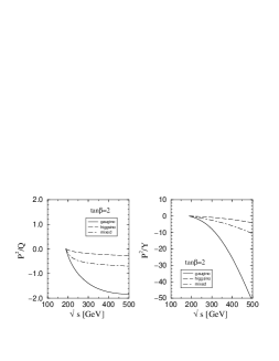
Figure 7: The energy dependence of the ratios ${\cal P}^{2}/{\cal Q}$ and ${\cal P}^{2}/{\cal Y}$ for the same set of parameters as for the cross section (23); solid line for the gaugino case, dashed line for the higgsino case, and dot-dashed line for the mixed case.

The observables ${\cal P}$, $\bar{\cal P}$, ${\cal Q}$ and ${\cal Y}$ enter into the cross section together with the spin analysis-power $\kappa(\bar{\kappa})$. CP–invariance leads to the relation $\bar{\kappa}=-\kappa$. Therefore, taking the ratios ${\cal P}^{2}/{\cal Q}$ and ${\cal P}^{2}/{\cal Y}$, these unknown quantities can be eliminated so that the two ratios reflect unambiguously the properties of the chargino system, being not affected by the neutralinos. It is thus possible to study the chargino sector in isolation by measuring the mass of the lightest chargino, the total production cross section and the spin(–spin) correlations. The energy dependence of the two ratios ${\cal P}^{2}/{\cal Q}$ and ${\cal P}^{2}/{\cal Y}$ is shown in Fig. 7; the same parameters are chosen as in the previous figures. The two ratios are sensitive to the quartic charges at sufficiently large c.m. energies since the charginos are, on the average, unpolarized at the threshold, c.f. eqs. (24). Note that ${\cal Y}$ vanishes for asymptotic energies so that an optimal energy must be chosen not far above threshold to measure this observable.

5. Observables and Extraction of SUSY Parameters

The pair production of the lightest chargino $\chi_{1}^{\pm}$ is characterized by the chargino mass $m_{\tilde{\chi}^{\pm}_{1}}$, the sneutrino mass $m_{\tilde{\nu}}$, and the two mixing angles $\cos 2\phi_{L,R}$. These three quantities can be determined from the production cross section and the spin correlations.

The mass $m_{\tilde{\chi}^{\pm}_{1}}$ can be measured very precisely near the threshold where the production cross section $\sigma(e^{+}e^{-}\rightarrow\tilde{\chi}^{+}_{1}\tilde{\chi}^{-}_{1})$ rises sharply with the velocity $\beta=\sqrt{1-4m_{\chi_{1}^{\pm}}^{2}/s}$. Combining the energy variation of the cross section with the measurement of the spin correlations, the sneutrino mass $m_{\tilde{\nu}}$ and the two mixing angles $\cos 2\phi_{L}$ and $\cos 2\phi_{R}$ can be extracted.

The decay angles $\{\theta^{*},\phi^{*}\}$ and $\{\bar{\theta}^{*},\bar{\phi}^{*}\}$, which are used to measure the $\chi_{1}^{\pm}$ chiralities, are defined in the rest frame of the charginos $\tilde{\chi}^{-}_{1}$ and $\tilde{\chi}^{+}_{1}$, respectively. Since there are two invisible neutralinos in the final state, they can not be reconstructed completely. However, the longitudinal components and the inner product of the transverse components can be reconstructed from the momenta measured in the laboratory frame (see e.g. Ref. [14]),

$$\cos\theta^{*}=\frac{1}{\beta|\vec{p}^{*}|}\left(\frac{E}{\gamma}-E^{*}\right)\ \ ,\ \ \cos\bar{\theta}^{*}=\frac{1}{\beta|\vec{\bar{p}}^{*}|}\left(\frac{\bar{E}}{\gamma}-\bar{E}^{*}\right)$$

$$\sin\theta^{*}\sin\bar{\theta}^{*}\cos(\phi^{*}+\bar{\phi}^{*})=\frac{|\vec{p}||\vec{\bar{p}}|}{|\vec{p}^{*}||\vec{\bar{p}}^{*}|}\cos\vartheta+\frac{\left(E-E^{*}/\gamma\right)\left(\bar{E}-\bar{E}^{*}/\gamma\right)}{\beta^{2}|\vec{p}^{*}||\vec{\bar{p}}^{*}|}$$ (59)

where $\gamma=\sqrt{s}/{2m_{\tilde{\chi}^{\pm}_{1}}}$. $E(\bar{E})$ and $E^{*}(\bar{E}^{*})$ are the energies of the two hadronic systems in the laboratory frame and in the rest frame of the charginos, respectively; $\vec{p}(\vec{\bar{p}})$ and $\vec{p}^{*}(\vec{\bar{p}^{*}})$ are the corresponding momenta. $\vartheta$ is the angle between the momenta of the two hadronic systems; the angle between the vectors in the transverse plane is given by $\Delta\phi^{*}=2\pi-(\phi^{*}+\bar{\phi}^{*})$ for the reference frames defined earlier. The polarization and correlation functions, ${\cal P}$, ${\cal Q}$ and ${\cal Y}$ can therefore be measured directly. Since the polarization ${\cal P}$ is odd under parity and charge–conjugation, it is necessary to identify the chargino electric charges in this case. This can be accomplished by making use of the mixed leptonic and hadronic decays of the chargino pairs. On the other hand, the observables ${\cal Q}$ and ${\cal Y}$ are defined without charge identification so that the dominant hadronic decay modes of the charginos can be exploited.

The measurements of the cross section at an energy $\sqrt{s}$, and either of the ratios ${\cal P}^{2}/{\cal Q}$ or ${\cal P}^{2}/{\cal Y}$ can be interpreted as contour lines in the plane $\{\cos 2\phi_{L},\cos 2\phi_{R}\}$ which intersect with large angles so that a high precision in the resolution can be achieved. A representative example for the determination of $\cos 2\phi_{L}$ and $\cos 2\phi_{R}$ is shown in Fig. 8. The mass of the light chargino is set to $m_{\tilde{\chi}^{\pm}_{1}}=95$ GeV, and the “measured” cross section, ${\cal P}^{2}/{\cal Q}$ and ${\cal P}^{2}/{\cal Y}$ are taken to be

$$\sigma(e^{+}e^{-}\rightarrow\tilde{\chi}^{+}_{1}\tilde{\chi}^{-}_{1})=0.37\ \ {\rm pb},\qquad\frac{{\cal P}^{2}}{\cal Q}=-0.24,\qquad\frac{{\cal P}^{2}}{\cal Y}=-3.66$$ (60)

at $\sqrt{s}=500$ GeV. The three contour lines meet at a single point $\{\cos 2\phi_{L},\cos 2\phi_{R}\}=\{-0.8,-0.5\}$ for $m_{\tilde{\nu}}=250$ GeV; note that the sneutrino mass can be determined together with the mixing angles from the “measured values” in eq. (60).

The solutions can be discussed most transparently by introducing the two triangular quantities

$$p=\cot(\phi_{R}-\phi_{L})\ \ {\rm and}\ \ q=\cot(\phi_{R}+\phi_{L})$$ (61)

They can be derived from the measured values $\cos 2\phi_{L}$ and $\cos 2\phi_{R}$ up to a discrete ambiguity which is due to the sign ambiguity in $\sin 2\phi_{L}$ and $\sin 2\phi_{R}$. Solving the set

$$p^{2}+q^{2} = \frac{2(\sin^{2}2\phi_{L}+\sin^{2}2\phi_{R})}{(\cos 2\phi_{L}-\cos 2\phi_{R})^{2}}$$

$$pq = \frac{\cos 2\phi_{L}+\cos 2\phi_{R}}{\cos 2\phi_{L}-\cos 2\phi_{R}}$$

$$p^{2}-q^{2} = \frac{4\sin 2\phi_{L}\sin 2\phi_{R}}{(\cos 2\phi_{L}-\cos 2\phi_{R})^{2}}$$ (62)

the solutions $(p,q)$ in point (1) and point (2) of Fig. 8 are found for $\sin 2\phi_{L}\sin 2\phi_{R}\stackrel{{\scriptstyle\textstyle>}}{{<}}0$, respectively. A second set is found by reversing the signs of the solutions pairwise. These solutions are shown for positive values of $pq$ in Fig. 8.

From the solutions $(p,q)$ derived above, the SUSY parameters can be determined in the following way.

(i) $\tan\beta$: Depending on the relative magnitude of $\cos 2\phi_{R}$ and $\cos 2\phi_{L}$, the value of $\tan\beta$ is either larger or smaller than unity. The first case is realized for

$$\cos 2\phi_{R}>\cos 2\phi_{L}\ \ :\ \ \tan\beta=\frac{p^{2}-q^{2}\pm 2\sqrt{\chi^{2}(p^{2}+q^{2}+2-\chi^{2})}}{(\sqrt{1+p^{2}}-\sqrt{1+q^{2}})^{2}-2\chi^{2}}\;\Rightarrow\;\tan\beta\geq 1$$ (63)

where $\chi^{2}=m^{2}_{\tilde{\chi}^{\pm}_{1}}/m^{2}_{W}$. If the denominator is positive, there are either up to two solutions for $\tan\beta>1$ in point (1) and none in point (2), or at most one in point (1) and at most one in point (2). The possible solutions can be counted in an analogous way if the denominator is negative; the rôles of point (1) and point (2) are just interchanged. The same counting is also valid in the second case for

$$\cos 2\phi_{R}<\cos 2\phi_{L}\ \ :\ \ \tan\beta=\frac{(\sqrt{1+p^{2}}-\sqrt{1+q^{2}})^{2}-2\chi^{2}}{p^{2}-q^{2}\pm 2\sqrt{\chi^{2}(p^{2}+q^{2}+2-\chi^{2})}}\;\Rightarrow\;\tan\beta\leq 1$$ (64)

Thus, only a two–fold ambiguity is inferred from all the solutions in point (1) and point (2).

(ii) $M_{2},\mu$: The gaugino and higgsino mass parameters are given in terms of $p$ and $q$ by the relations

$$M_{2} = \frac{m_{W}}{\sqrt{2}}\bigg{[}(p+q)\sin\beta-(p-q)\cos\beta\bigg{]}$$

$$\mu = \frac{m_{W}}{\sqrt{2}}\bigg{[}(p-q)\sin\beta-(p+q)\cos\beta\bigg{]}$$ (65)

The parameters $M_{2}$, $\mu$ are uniquely fixed if $\tan\beta$ is chosen properly in point (1) and/or point (2). Since $\tan\beta$ is invariant under pairwise reflection of the signs in $(p,q)$, the definition $M_{2}>0$ can be exploited to remove this additional ambiguity.

As a result, the fundamental SUSY parameters [$\tan\beta;M_{2},\mu$] can be derived from the observables $m_{\tilde{\chi}^{\pm}_{1}}$ and $\cos 2\phi_{R}$, $\cos 2\phi_{L}$ up to at most a two–fold ambiguity.

Returning to the “experimental values” of mass, cross section and spin correlations introduced above, the following SUSY parameters are extracted:

$${\rm Point\ \ (2)}\;:\;[\tan\beta;M_{2},\mu]=\left\{\begin{array}[]{l}[1.06;\;83{\rm GeV},\;-59{\rm GeV}]\\ {}\\ {}[3.33;\;248{\rm GeV},\;123{\rm GeV}]\end{array}\right.$$ (69)

Two solutions are derived from the “experimental values” in this case; point (1) gives negative values for $\tan\beta$. In practice, the errors in the observables $m_{\tilde{\chi}^{\pm}_{1}}$ and $\cos 2\phi_{R,L}$ must be analyzed experimentally and the migration to the fundamental SUSY parameters must be studied properly. This however is beyond the scope of the purely theoretical analysis presented in this paper.

6. Conclusions

We have analyzed how the parameters of the chargino system, the mass of the lightest chargino $m_{\tilde{\chi}^{\pm}_{1}}$ and the size of the wino and higgsino components in the chargino wave–functions, parameterized in terms of the two angles $\phi_{L}$ and $\phi_{R}$, can be extracted from pair production of the lightest chargino state in $e^{+}e^{-}$ annihilation. In addition to the total production cross section, angular correlations among the chargino decay products give rise to two independent observables which can be measured directly despite of the two invisible neutralinos in the final state.

From the chargino mass $m_{\tilde{\chi}^{\pm}_{1}}$ and the two mixing angles $\phi_{L}$ and $\phi_{R}$, the fundamental supersymmetric parameters $\tan\beta$, $M_{2}$ and $\mu$ can be extracted up to at most a two-fold discrete ambiguity. Moreover, from the energy distribution of the final particles in the decay of the chargino, the mass of the lightest neutralino can be measured; this allows to determine the parameter $M_{1}$ so that also the neutralino mass matrix can be reconstructed in a model-independent way.

The analysis has been carried out for scenarios in which the chargino sector is CP–invariant. The generalization to CP non–invariant theories [12, 15] is touched upon in a brief appendix for completeness.

Acknowledgments

This work was supported by the KOSEF-DFG large collaboration project, Project No. 96-0702-01-01-2, and by the Polish State Committee for Scientific Research, Grant No. 2 P 03B 030 14. Thanks go to M. Raidal for comments on the manuscript.

APPENDIX: Complex mass parameters

In CP–noninvariant theories, the gaugino mass $M_{2}$ and the Higgs mass parameter $\mu$ can be complex. However, by reparametrizations of the fields, $M_{2}$ can be assumed real and positive without loss of generality [12] so that the only non–trivial invariant phase is attributed to $\mu$:

$$\mu=|\mu|{\rm e}^{i\theta}$$ (70)

In these theories the complex chargino mass matrix (3) is diagonalized by two unitary matrices $U_{L}$ and $U_{R}$:

$$U_{L,R}\left(\begin{array}[]{c}\tilde{W}^{-}\\ \tilde{H}^{-}\end{array}\right)_{L,R}=\left(\begin{array}[]{c}\tilde{\chi}^{-}_{1}\\ \tilde{\chi}^{-}_{2}\end{array}\right)_{L,R}$$ (75)

They can be parameterized in the following way:

$$U_{L}=\left(\begin{array}[]{cc}\cos\phi_{L}&{\rm e}^{-i\beta_{L}}\sin\phi_{L}\\ -{\rm e}^{i\beta_{L}}\sin\phi_{L}&\cos\phi_{L}\end{array}\right)$$ (78)

$$U_{R}=\left(\begin{array}[]{cc}{\rm e}^{i\gamma_{1}}&0\\ 0&{\rm e}^{i\gamma_{2}}\end{array}\right)\left(\begin{array}[]{cc}\cos\phi_{R}&{\rm e}^{-i\beta_{R}}\sin\phi_{R}\\ -{\rm e}^{i\beta_{R}}\sin\phi_{R}&\cos\phi_{R}\end{array}\right)$$ (83)

The eigenvalues $m^{2}_{\tilde{\chi}^{\pm}_{1}}$ involve the angle $\theta$:

$$m^{2}_{\tilde{\chi}^{\pm}_{1,2}}=\frac{1}{2}\bigg{[}M_{2}^{2}+|\mu|^{2}+2m^{2}_{W}\mp\Delta_{C}\bigg{]}$$ (84)

with

$$\Delta_{C}=\sqrt{(M_{2}^{2}+|\mu|^{2}+2m^{2}_{W})^{2}-4(M_{2}^{2}|\mu|^{2}-2m^{2}_{W}M_{2}|\mu|\sin 2\beta\cos\theta+m^{4}_{W}\sin^{2}2\beta)}$$ (85)

The four nontrivial phase angles $\{\beta_{L},\beta_{R},\gamma_{1},\gamma_{2}\}$ also depend on the invariant angle $\theta$:

$$\tan\beta_{L}=-\frac{\sin\theta}{\cos\theta+\frac{M_{2}}{|\mu|}\cot\beta} \tan\beta_{R}=+\frac{\sin\theta}{\cos\theta+\frac{M_{2}}{|\mu|}\tan\beta}$$ ,

$$\tan\gamma_{1}=+\frac{\sin\theta}{\cos\theta+\frac{M_{2}}{|\mu|}\frac{m^{2}_{\tilde{\chi}^{\pm}_{1}}-|\mu|^{2}}{m^{2}_{W}\sin 2\beta}} \tan\gamma_{2}=-\frac{\sin\theta}{\cos\theta+\frac{M_{2}}{|\mu|}\frac{m^{2}_{W}\sin 2\beta}{m^{2}_{\tilde{\chi}^{\pm}_{2}}-M_{2}^{2}}}$$ , (86)

The mixing angles $\phi_{LR}$ are given by the relations

$$\cos 2\phi_{L}=-\frac{M_{2}^{2}-|\mu|^{2}-2m^{2}_{W}\cos 2\beta}{\Delta_{C}}$$

$$\sin 2\phi_{L}=-\frac{2m_{W}\sqrt{M_{2}^{2}+|\mu|^{2}+(M_{2}^{2}-|\mu|^{2})\cos 2\beta+2M_{2}|\mu|\sin 2\beta\cos\theta}}{\Delta_{C}}$$

and

$$\cos 2\phi_{R}=-\frac{M_{2}^{2}-|\mu|^{2}+2m^{2}_{W}\cos 2\beta}{\Delta_{C}}$$

$$\sin 2\phi_{R}=-\frac{2m_{W}\sqrt{M_{2}^{2}+|\mu|^{2}-(M_{2}^{2}-|\mu|^{2})\cos 2\beta+2M_{2}|\mu|\sin 2\beta\cos\theta}}{\Delta_{C}}$$ (87)

The $\tilde{\chi}_{1}\tilde{\chi}_{1}\gamma$ and $\tilde{\chi}_{1}\tilde{\chi}_{1}Z$ vertices are real and they can be expressed by the mixing angles $\phi_{L,R}$ in the same way as in CP–invariant theories. Even though the new phases enter the $e\tilde{\nu}\tilde{\chi}_{1}$ vertex, they do not affect the $\tilde{\nu}$–exchange amplitude. As a result, the analytical expressions of all observables in the diagonal process $e^{+}e^{-}\rightarrow\tilde{\chi}^{+}_{1}\tilde{\chi}^{-}_{1}$ remain the same when described in terms of the mixing angles $\phi_{L}$ and $\phi_{R}$. Since the density matrix (31) is factored out completely and the form of the sixteen coefficients in eqs. (41), (42) and (43) does not change by CP-noninvariance, the analysis described in this paper is not changed.

If the phase $\theta$ is introduced, the observables $m_{\tilde{\chi}^{\pm}_{1}},\phi_{L}$ and $\phi_{R}$ are insufficient to reconstruct the fundamental SUSY parameters $\tan\beta$, $M_{2}$, $|\mu|$ and $\theta$ in toto. In this complex situation, one more observable is needed. The additional information may be extracted, for example, from the $\tilde{\chi}^{\pm}_{2}$ mass. [Else the neutralino system may be exploited to provide the additional observable [15]]. The CP–odd phase $\theta$ can be determined directly in the non–diagonal process $e^{+}e^{-}\rightarrow\tilde{\chi}^{+}_{1}\tilde{\chi}^{-}_{2}$, see Ref. [12].

Figure 2: The cross section for the production of charginos, (a) as a function of the c.m. energy with $m_{\tilde{\nu}}=200$ GeV, and (b) as a function of the sneutrino mass with $\sqrt{s}=200$ GeV for the representative set of SUSY parameters in eq. (23): solid line for the gaugino case, dashed line for the higgsino case, and dot-dashed line for the mixed case.

Figure 3: The angular distribution as a function of the scattering angle at c.m. energies (a) 200 and (b) 500 GeV for the set of SUSY parameters in eq. (23) and $m_{\tilde{\nu}}=200$ GeV.

Figure 4: The angular dependence of the longitudinal polarization ${\cal P}_{L}$ and the transverse polarization ${\cal P}_{T}$ for the same parameters as for the cross section (23) at c.m. energies (a) 200 and (b) 500 GeV; solid line for the gaugino case, dashed line for the higgsino case, and dot-dashed line for the mixed case.

Figure 6: The polarization analysis–power $\kappa$ as a function of the hadron invariant mass $\sqrt{s^{\prime}}$ for the same set of parameters as for the cross section (23).

Figure 8: Determination of $(p,q)$ from $p^{2}+q^{2}$, $pq$ and $p^{2}-q^{2}$. The solutions are illustrated for positive values of $pq$.

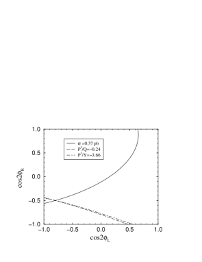
Figure 9: Contours for the “measured values” (60) of the total cross section (solid line), ${\cal P}^{2}/{\cal Q}$ (dashed line), and ${\cal P}^{2}/{\cal Y}$ (dot-dashed line) for $m_{{\chi}^{\pm}_{1}}=95$ GeV [$m_{\tilde{\nu}}=250$ GeV].

References

- [1] For reviews of supersymmetry and the Minimal Supersymmetric Standard Model, see H. Nilles, Phys. Rep. 110 (1984) 1; H.E. Haber and G.L. Kane, Phys. Rep. 117 (1985) 75.
- [2] J. Ellis, J. Hagelin, D. Nanopoulos and M. Srednicki, Phys. Lett. 127B (1983) 233; V. Barger, R.W. Robinett, W.Y. Keung and R.J.N. Phillips, Phys. Lett. B131 (1983) 372; D. Dicuss, S. Nandi, W. Repko and X. Tata, Phys. Rev. Lett. 51 (1983) 1030; S. Dawson, E. Eichten and C. Quigg, Phys. Rev. D31 (1985) 1581; A. Bartl and H. Fraas and W. Majerotto, Z. Phys. C30 (1986) 441.
- [3] Proceedings of the Workshop on Physics at LEP II, Report No. CERN-96-01, eds. G. Altarelli, T. Sjöstrand, and F. Zwirner.
- [4] E. Accomando et al., LC CDR Report DESY 97-100 (hep-ph/9705442), and Physics Reports 299 (1998) 1.
- [5] S.Y. Choi, YUMS 98-3 (hep-ph/9801323); Talk at The First Workshop: Pacific Particles Physics Phenomenology, Seoul 1997.
- [6] A. Leike, Int. J. Mod. Phys. A3 (1988) 2895; M.A. Diaz and S.F. King, Phys. Lett. B349 (1995) 105; B373 (1996) 100; J.L. Feng and M.J. Strassler, Phys. Rev. D51 (1995) 4461 and D55 (1997) 1326; G. Moortgat-Pick and H. Fraas, Report WUE-ITP-97-026 (hep-ph/9708481).
- [7] G. Moortgat-Pick, H. Fraas, A. Bartl and, and W. Majerotto, WUE-ITP-98-012 (hep-ph/9804306).
- [8] L.M. Sehgal and P.M. Zerwas, Nucl. Phys. B183 (1981) 417.
- [9] K. Hagiwara and D. Zeppenfeld, Nucl. Phys. B274 (1986) 1.
- [10] L. Michel and A.S. Wightman, Phys. Rev. 98 (1955) 1190; C. Bouchiat and L. Michel, Nucl. Phys. 5 (1958) 416; S.Y. Choi, Taeyeon Lee and H.S. Song, Phys. Rev. D40 (1989) 2477.
- [11] J.H. Kühn, A. Reiter and P.M. Zerwas, Nucl. Phys. B272 (1986) 560.
- [12] Y. Kizukuri and N. Oshimo, Proceedings of the Workshop on Collisions at 500 GeV: The Physics Potential, Munich-Annecy-Hamburg 1991/93, DES 92-123A+B, 93-123C, ed. P. Zerwas; T. Ibrahim and P. Nath, Phys. Rev. D57 (1998) 478; S.Y. Choi and M. Drees, in preparation.
- [13] A. Datta, M. Guchait and M. Drees, Z. Phys. C69 (1996) 347.
- [14] J.H. Kühn and F. Wagner, Nucl. Phys. B236 (1994) 16.
- [15] M. Brhlik and G.L. Kane, hep-ph/9803391.