Study of Nondiagonal Parton Distribution Models
Abstract
In this paper we examine predictions from different models of nondiagonal
parton distributions. This will be achieved by examining whether certain
predictions of relationships between diagonal and nondiagonal parton
distributions also hold after having evolved the different distributions.
PACS: 12.38.Bx, 13.85.Fb, 13.85.Ni
Keywords: Deeply Virtual Compton Scattering, Nondiagonal distributions,
Evolution
I Introduction
In recent years deeply virtual Compton scattering (DVCS), hard exclusive electroproduction processes and the distributions which contain the nonperturbative information for those processes, namely the nondiagonal or nonforward parton distributions, together with their evolution have been a target of intense studies [1, 2, 3, 4, 5, 6, 7, 8, 9, 10, 11, 12, 13, 14, 15, 16, 17, 18, 19, 20, 21].
Nondiagonal parton distributions, in particular, have attracted a lot of attention and numerical studies as to their behavior under their leading order (LO) evolution were conducted recently [5, 6, 7]. Also recently, the next-to-leading order (NLO) generalized Efremov-Radyushkin-Brodsky-Lepage anomalous dimensions were computed employing conformal symmetry arguments [13] making NLO studies in the near future possible. The NLO kernels for the DGLAP region () of the nondiagonal parton distributions can be reconstructed via the method described in Ref. [22].
In the above mentioned numerical studies, a particular ansatz for the initial distribution for nondiagonal evolution was made, namely that the nondiagonal and diagonal initial distributions were taken to be equal in the normalization point. As was pointed out in [23] this ansatz cannot be justified except at very low normalization point where the parton distributions are essentially flat. In the following, we will explore a different ansatz and investigate whether predictions based on this ansatz hold after evolution. It is crucial for the predictive power of theoretical calculations of exclusive, hard diffractive processes to have sensible nonperturbative models of nondiagonal parton distributions as long as they have not been extracted from experiment.
The paper is structured the following way. In Sec. II we recap a few basic definitions about nondiagonal parton distributions and the involved kinematics, in Sec. III we will briefly explain the model under consideration as derived by Radyushkin [23] and the predictions about the relationship between nondiagonal and diagonal parton distributions, in Sec. IV we will give the results of our study, making some remarks about the behavior of nondiagonal parton distributions in NLO and, finally, in Sec. V we give concluding remarks.
II Basics
The kinematics as encountered in the appearance of nondiagonal parton distributions can be most easily described by the DVCS process . The fact that the initial and final state protons have different momenta leads to the introduction of nondiagonal parton distributions. The nondiagonal character of these distributions can be seen in the definitions of nondiagonal parton distributions as Fourier transforms of matrix elements of bilocal, renormalized light-cone operators (see Ref. [2, 3, 4] and below) , the light-cone operators being sandwiched between states of different momenta as compared to the diagonal case where the states have the same momentum.

The important kinematical parameters are the following: is the virtuality of the probing photon, is the momentum transfer to the final state proton, is the usual Bjorken scaling variable, is the asymmetry parameter of the process and and are the longitudinal light-cone momentum fractions of the partons connecting the intermediate state to the hard scattering part (see Fig. 1). Note that in the case of DVCS .
For our study we need the definitions of nondiagonal parton distributions in terms of light-cone operators, their evolution equations and LO evolution kernels which we will review next.
III Radyushkin’s model
In the following we will briefly review the simplest model for an initial nondiagonal parton distribution as proposed by Radyushkin in Ref. [23]. The starting point are double distributions which behave like a distribution amplitude in the variable and like a parton distribution in the variable . They are expressed through multivariable Fourier transforms of matrix elements of bilocal, renormalized, light-cone operators [2, 23]. Symmetry and spectral conditions suggest the following ansatz for the double distribution [23]
| (11) |
such that with the normalization condition
| (12) |
one obtains the diagonal distribution
| (13) |
The simplest realization of the ansatz Eq. (11) is [23]
| (14) |
The -function in prevents any spread of the double distribution in the direction and is a number smaller than and is determined by the powerlaw behavior of parton densities at small .
In order to obtain the nondiagonal parton distribution in the DGLAP region () from the double distribution, one has to integrate over with an explicit dependence
| (15) |
Using Eq. (14) one finds the following initial distribution which will be our input for the evolution
| (16) |
with and we chose which is in line with the arguments in [23] that the crest of the double distribution is shifted towards the line . Note that the ansatz of the previous numerical studies [5, 8] was that the diagonal and nondiagonal distributions were equal in the normalization point which corresponds to a double distribution similar to Eq. (14) with .
The above made ansatz leads to the following predictions (see Ref. [23] for more details) for nondiagonal parton distributions:
| (17) |
and
| (18) |
The first equation is of importance in the case of DVCS since there one has . The second equation supposedly holds for any . If the above predictions hold true even after evolution it would give a very useful approximation of nondiagonal parton densities.
IV Results of Evolution
Our input distributions for the diagonal parton densities in Eq. (14) will be CTEQ4M and CTEQ4LQ [24]. The reason why we chose these distributions is simple. Both CTEQ4M at a fairly high normalization point of and CTEQ4LQ at a very low normalization point of are discernably different in the initial shape. This will help us discriminate fairly easily how robust to the initial shape the predictions of the previous section are.
Our input distributions for the nondiagonal evolution are those satisfying relation (16). Since the nondiagonal evolution kernels are known explicitly to leading order (LO) only, we only use LO kernels for the diagonal evolution also, in order to have a consistent comparison between the nondiagonal and diagonal case.
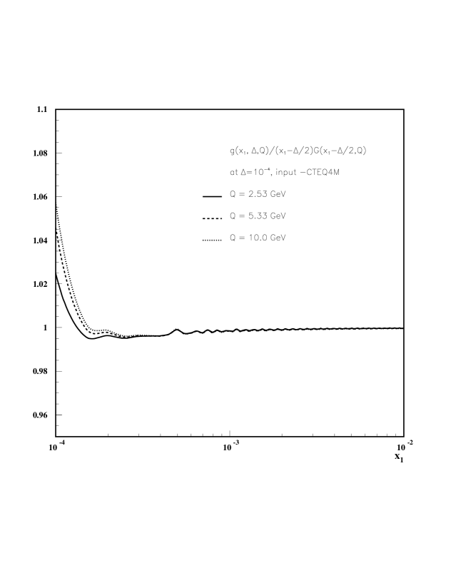
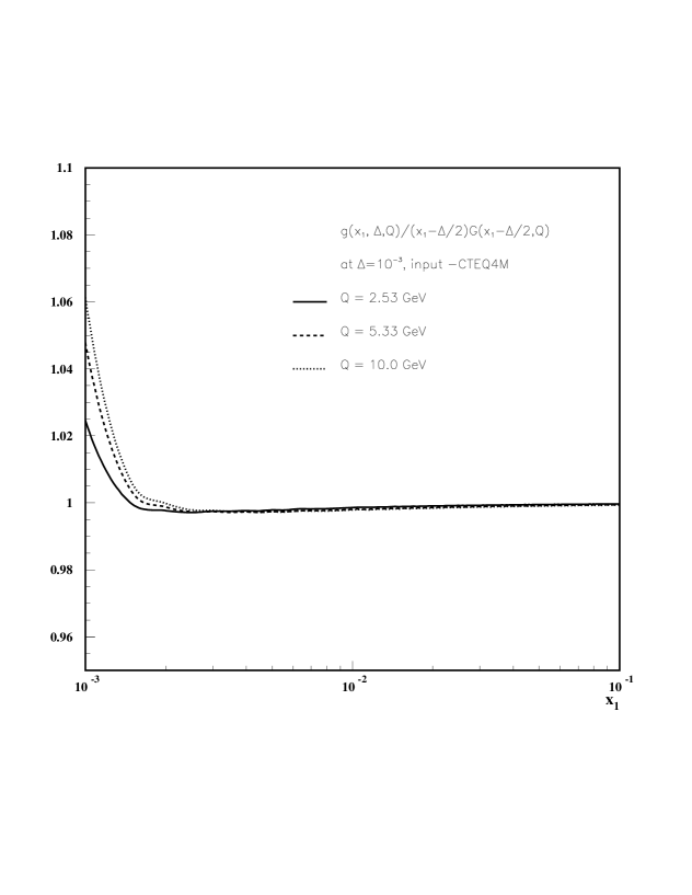
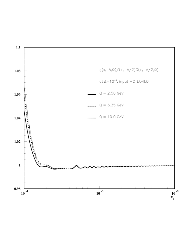
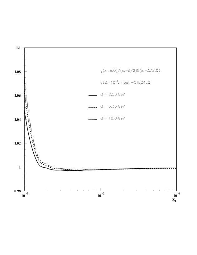
Let us first discuss how well Eq. (18) is satisfied. The results of our numerical study are given in Figs. (3,4,5,6). Although the input distribution for the nondiagonal evolution was chosen according to Eq. (18) at , the evolution hardly violates this relationship at . One can see from Figs. (3,4) that as the nondiagonal density evolves with the ratio of the nondiagonal to diagonal gluon parton density stays within for all and , for both CTEQ4M and CTEQ4LQ. Note that in these figures . As increases the difference between the nondiagonal and diagonal densities becomes small. This is a natural behaviour of the nondiagonal densities since for all the asymmetry related effects are unimportant.
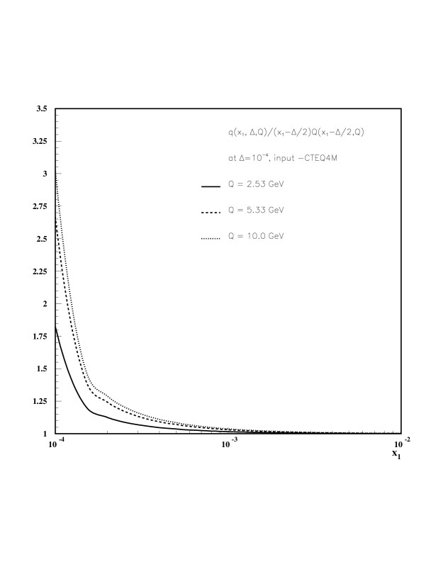
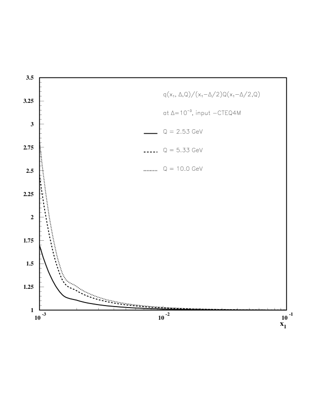
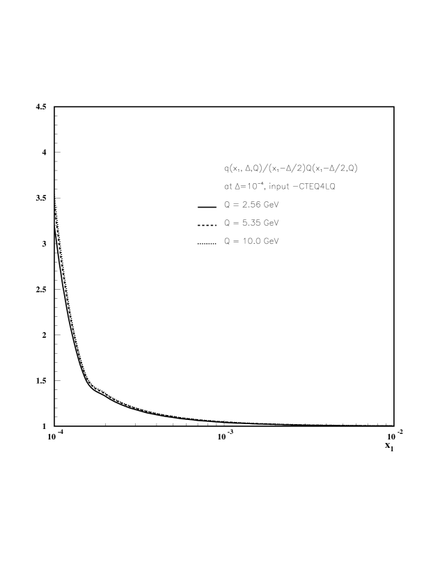
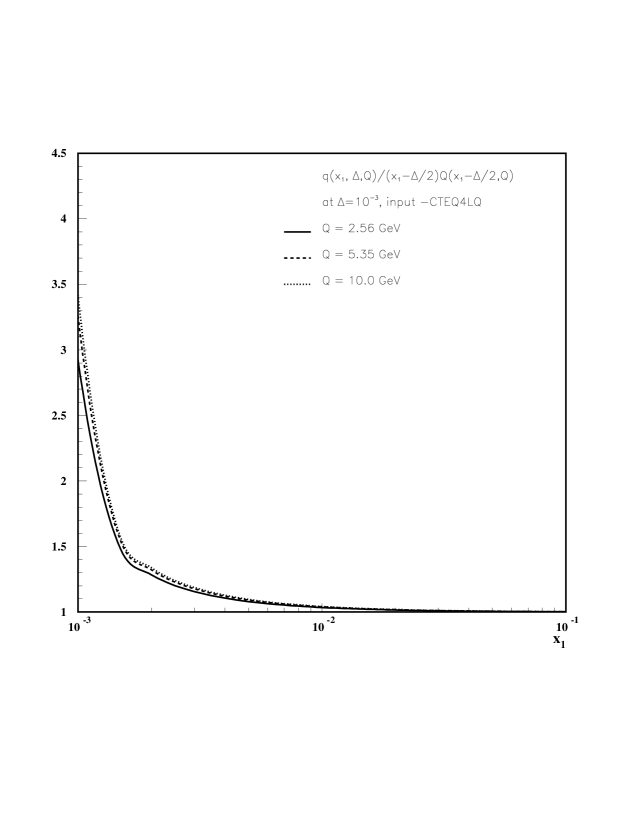
Next, we present the ratio of the nondiagonal to diagonal quark parton
densities
in Figs. (5,6). The quark parton density is defined
| (19) |
Here we observe a similar tendency as in the case of gluons – at close to – the difference between the nondiagonal and diagonal densities is different from . However, in the case of quarks the ratio is significantly larger than . In fact, the nondiagonal quark is about times larger than the diagonal one at (here ) ***The same behaviour was observed by Golec-Biernat [25]. This result is not too surprising, in light of the findings of Ref. [7], which showed a large deviation of the nondiagonal quark distribution from the diagonal one for with a strong enhancement in the deviation for a low normalization point. As becomes significantly large than the ratio quickly and smoothly approaches , as expected.
To summarize this set of figures, we conclude that the prescription of Eq. (18), where one shifts the argument of the diagonal parton density by , decreases the percentage deviation of the nondiagonal to diagonal parton density by approximately a factor of for gluons (compare to the relevant figures from Ref. [7]), giving a very good agreement for all and . For quarks the approximation of Eq. (18) is much worse as compared to the gluon case, however it becomes relatively good for to .
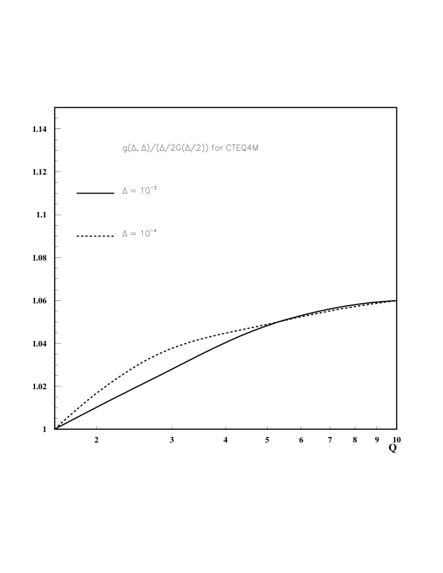
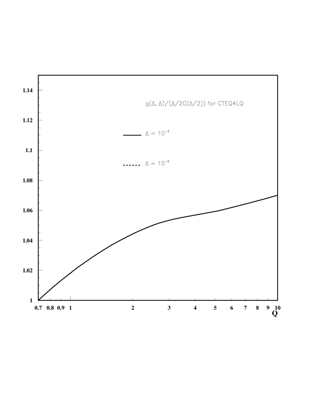
Next we find that Eq. (17) is fulfilled with an accuracy better than in the and range studied for both CTEQ4M and CTEQ4LQ (see Fig. 2). This is very good as far as DVCS studies are concerned since Eq. (17) is an all order statement and thus one can use the NLO evolution of diagonal gluon densities to make NLO predictions for DVCS! As mentioned before, we have chosen for and for . As one can see there is no big difference in the ratio of the densities for the two values studied which is in agreement with Radyushkin’s statement that Eq. (17) should hold as long as is much smaller than .
Finally, we would like, in light of the previous findings, comment on the NLO evolution in the DGLAP region. Given the fact that Eq. (17,18) was based on general arguments in [23] and that it holds in LO evolution with a certain degree of accuracy, we predict that the NLO evolution will not change the above relations, in other words, that the NLO evolution of the nondiagonal gluon distribution can be predicted to a similar accuracy by the NLO evolution of the diagonal gluon distribution. We base this statement on the results of the above analysis and the observations of [7] that the NLO corrections of the nondiagonal evolution should be in the same direction as in the diagonal case, which reduces the LO results, and of the same magnitude. The former statement is due to the observations made in [7] that if, in the nondiagonal case, the NLO corrections were in the opposite direction, which would lead to a marked deviation from the LO results, compared to the diagonal case, the overall sign of the NLO nondiagonal kernels would have to change for some since in the limit we have to recover the diagonal case. This occurance is not likely for the following reason: First, the Feynaman diagrams involved in the calculation of the NLO nondiagonal kernels are the same as in the diagonal case, except for the different kinematics, therefore, we have a very good idea about the type of terms appearing in the kernels, namely polynomials, logs and terms in need of regularization such as . Secondly, the kernels, as stated before, have to reduce to the diagonal case in the limit of vanishing which fixes the sign of most terms in the kernel, thus the only type of terms which are allowed and could change the overall sign of the kernel are of the form
| (20) |
which will be numerically small unless in the convolution integral of the evolution equations. Moreover, we know that in this limit the contribution of the regularized terms in the kernel gives the largest contributions in the convolution integral and therefore sign changing contributions in the nondiagonal case would have to originate from regularized terms. This in turn disallows a term like Eq. 20 due to the fact that regularized terms are not allowed to vanish in the diagonal limit, since the regularized terms arise from the same Feynman diagrams in the both diagonal and nondiagonal case. Therefore, the overall sign of the contribution of the NLO nondiagonal kernels will be of the same as in the diagonal case . In addition, the magnitude of the correction should be of the same magnitude as in the diagonal case since one has the conditions [6, 20, 23], [23] for the gluon distribution and the fact that the LO results at high are already fairly close to the upper bound. This forces the NLO corrections in the nondiagonal case not to exceed the diagonal corrections by a factor of or so, lest it violates the boundary conditions for .
V Conclusions
In the above, we examined predictions made in Ref. [23] about relationships between nondiagonal and diagonal parton distributions in the DGLAP region based on certain models for nondiagonal parton distributions in the normalization point. We found that the evolution does not destroy the validity of Eqs. (17,18) for all and for both CTEQ4M and CTEQ4LQ in the case of gluons and for for quarks. Therefore, we conclude that Eqs. (17,18) do supply a reliable approximation of nondiagonal parton densities for . We also conclude that we can hardly see a variance of the accuracy of predictions (17,18) for different initial distributions. The accuracy is slightly better for the one which supplies a less steep gluon density at small .
Based on these results and the results from Ref. [7], we predicted the NLO evolution of the nondiagonal gluon distribution to be within of the diagonal gluon distribution for the above made ansatz and for a large range of .
Acknowledgments
This work was supported in part by the U.S. Department of Energy under grant number DE-FG02-90ER-40577. We would like to thank John Collins, Mark Strikman and Anatoly Radyushkin for helpful conversations and once more Anatoly Radyushkin for pointing out an inconsistency in an earlier draft version due to a minor error in our evolution code.
We also would like to thank Martin McDermott who has drawn our attention to an error in the input of the initial quark parton densities in our evolution code. This forced us to review the numerical results and figures of this paper and our previous one [7].
After this work was complete, we learned that Müller et al. [26] had performed a numerical study of the NLO effects for the non-singlet and singlet distributions and found that the corrections were within percent of the LO result confirming our statements on the NLO corrections.
REFERENCES
- [1] S.J. Brodsky, L.L. Frankfurt, J.F. Gunion, A.H. Mueller, and M. Strikman, Phys. Rev. D50 (1994) 3134; ibid. Erratum in print
- [2] A. Radyushkin Phys. Letters B385 (1996) 333, Phys.Lett B380 (1996) 417, Phys. Rev. D56, 5524 (1997).
- [3] J.C. Collins, L. Frankfurt, and M. Strikman, Phys. Rev. D56 (1997) 2982.
- [4] X.-D. Ji, Phys. Rev. D55 (1997) 7114, Phys. Rev. Lett. 78, 610 (1997).
- [5] L.L. Frankfurt, A. Freund, V. Guzey and M. Strikman, Phys. Lett. B 418, 345 (1998).
- [6] A.Martin and M.Ryskin, Phys. Rev. D57, 6692 (1998).
- [7] A. Freund and V. Guzey, hep-ph/9801388.
- [8] L. Mankiewicz, G. Piller and T. Weigel, hep-ph/9711227.
- [9] J.C. Collins and A. Freund, hep-ph/9801262.
- [10] X.-D. Ji and J. Osborne, hep-ph/9801260.
- [11] D. Müller, “Restricted conformal invariance in QCD and its predictive power for virtual photon processes”, hep-ph/9704406.
- [12] X. Ji and J. Osborne, Phys. Rev. D57, 1337 (1998).
- [13] A.V. Belitsky and D. Müller, Phys. Lett. B417, 129 (1998), hep-ph/9802411, hep-ph/9804379.
- [14] A.V. Belitsky, B. Geyer, D. Müller, A. Schäfer Phys. Lett. bf B421, 312 (1998).
- [15] M. Diehl, T. Gousset, B. Pire, and J.P. Ralston, Phys. Lett. B411, 193 (1997),
- [16] Z. Chen, “Non-Forward and Unequal Mass Virtual Compton Scattering” , hep-ph/9705279.
- [17] L. Frankfurt, A. Freund and M. Strikman, hep-ph/9710356 to appear in Phys. Rev. D.
- [18] L. Mankiewicz, G. Piller, E. Stein, M. Vättinen and T. Weigl, “NLO Corrections to Deeply-Virtual Compton Scattering”, hep-ph/9712251.
- [19] J. Blümlein, B. Geyer, and D. Robaschik, Phys. Lett. B406, 161 (1997), hep-ph/9711405.
- [20] B. Pire, J. Soffer and O. V. Teryaev, hep-ph/9804284.
- [21] L. Frankfurt, A. Freund and M. Strikman preprint in preparation.
- [22] F. M. Dittes, J. Horejsi, B. Geyer, D. Müller and D. Robaschick, Phys. Lett. B209, 325 (1988).
- [23] A. Radyushkin, hep-ph/9805342.
- [24] H. Lai et al., Phys. Rev. D55, 1280 (1997).
- [25] K. Golec-Biernat, private communications.
- [26] A. V. Belitsky, D. Müller, L. Niedermeier and A. Schäfer, hep-ph/9806232 and hep-ph/9810275.