Abstract

We present ${\cal O}(\alpha_{s}^{2})$ corrections to the decay $t\to bW$ in the limit of a very large top quark mass, $m_{t}\gg m_{W}$. We find that the ${\cal O}(\alpha_{s}^{2})$ effects decrease the top quark decay width $\Gamma_{t}$ by about 2%: $\Gamma_{t}=\Gamma_{0}(1-0.8\alpha_{s}(m_{t})-1.7\alpha_{s}^{2})$. The complete corrections are smaller by about 24% than their estimate based on the BLM effects ${\cal O}(\beta_{0}\alpha_{s}^{2})$. We explain how to compute a new type of diagrams which contribute to $\Gamma(t\to bW)$ at the ${\cal O}(\alpha_{s}^{2})$ level.

1 Introduction

Because of its very large mass, the top quark is an interesting object for precise studies and searches for possible “new physics.” In consequence of the large $m_{t}$, top lifetime is very short. With good accuracy the top decay rate $\Gamma_{t}$ is proportional to the third power of the top mass and equals approximately $1.5$ GeV for $m_{t}=175$ GeV. This large width makes the top quark behave almost like a free quark, a unique situation in QCD [1]. The reason for this is that the time scale $\tau_{W}$ of the weak top quark decay

$$\tau_{W}\approx\left[\frac{G_{F}m_{t}^{3}}{8\sqrt{2}\pi}\right]^{-1},$$

is much shorter than the time scale of the non-perturbative QCD effects, $1/\Lambda_{\rm QCD}$.

Within the Standard Model (SM) the reaction $t\to bW$ is the dominant top quark decay channel. However, in most extensions of the standard model (SM) there are additional decay channels (e.g. $t\to bH^{+}$ or decays into final states including supersymmetric particles). Since the SM prediction for the top quark lifetime can be given with high precision, its measurements can in principle shed light on the new physics contributions to top decay.

The fact that the life time of the top quark is so small has rather interesting consequences for the top production in $e^{+}e^{-}$ annihilation. Because the nonperturbative effects are suppressed by the large $\Gamma_{t}$, threshold production cross section of $t\bar{t}$ in $e^{+}e^{-}$ collisions can be predicted rather reliably. Clean signature and a rich physics potential [2] make the investigation of this process in the threshold region one of the priorities at the Next Linear Collider (NLC). Many studies have recently been performed in order to describe this reaction with high precision (see e.g. [3, 4, 5]).

The total cross section for $e^{+}e^{-}\to t\bar{t}$ in the threshold region is determined by the equation:

$$\sigma_{t}(s)\sim{\rm Im}\;G(E+i\Gamma_{t};0,0),$$ (1)

where $s$ is the center of mass energy squared, $E\equiv\sqrt{s}-2m_{t}$, and $G(E;0,0)$ is the value at the origin of the Schrödinger equation Green function describing the non–relativistic $t\bar{t}$ system. Because of the $\sigma_{t}(s)$ dependence on $\Gamma_{t}$, a precise prediction for the cross section requires a matching accuracy in $\Gamma_{t}$. This is true not only for the total cross section but also for other top threshold observables, for example top momentum distribution.

The analysis of $\sigma_{t}(s)$ has been recently extended to the next-to-next-to-leading order accuracy [4, 5]. That analysis was made possible in part by the recently calculated two-loop corrections to the QCD potential [6], whose influence on the threshold cross section was investigated in [7]. On the other hand, the ${\cal O}(\alpha_{s}^{2})$ corrections to the width were not known at that time and were not included into those studies. The purpose of the present paper is to provide $\Gamma_{t}$ including ${\cal O}(\alpha_{s}^{2})$ effects.

The direct measurement of the top quark decay width at NLC is difficult. At the moment a determination of the top quark width based on the measurement of the forward-backward asymmetry of $t$ quarks in the threshold region in $e^{+}e^{-}$ collisions is considered to be the most promising option. It is believed that the accuracy of $10-20\%$ can be obtained in such a measurement [2]. More optimistic estimates of 5% accuracy have also been published [8]. Still better accuracy might be obtained at a future muon collider.

Because of the importance of the top quark width, much effort has been invested into studies of radiative corrections to its decays. Here we briefly summarize the results obtained in the SM. For a more extensive discussion and a summary of calculations in some extensions of the SM we refer the reader to ref. [9, 10], where also corrections to various differential decay distributions are presented.

QCD corrections to heavy quark decays were first studied in an effective Fermi-like theory, valid for quarks much lighter than the $W$ [11]. For the semileptonic decays such calculations were technically similar to the muon decay case [12]. After it had become clear that the top quark is heavy, QCD corrections were calculated in [13] with full $W$ propagator taken into account. These results are also applicable to the process $t\to bW$ which is now considered the dominant decay channel of the top quark, and in this context were confirmed in [14]. The one-loop QCD corrections decrease the rate of this decay by about $-8.4\%$ (for $m_{t}\approx 175$ GeV).

At the ${\cal O}(\alpha_{s}^{2})$ level only the so-called BLM [15] corrections have been known [16, 17]. Their numerical value will be illustrated below. Summation of these effects to all orders has been discussed in [18, 19].

The electroweak corrections to $t\to bW$ were evaluated in [20] and were found to increase the decay rate by about 1.7%. This effect is almost canceled by accounting for the finite width of the $W$, which decreases the rate by about $-1.5\%$ [10]. In the present paper these both effects will be neglected.

Present uncertainty in the theoretical prediction of the top quark width is to a large extent connected with the unknown two-loop QCD corrections [9] and the need for their complete evaluation has been repeatedly emphasized. This paper is devoted to this calculation. An exact computation of this effect would be very difficult, but since the size of those corrections is expected to be small, it is justified to make some approximations. In the present calculation we neglect the mass of the $W$; the error is expected to be of the order $m_{W}^{2}/m_{t}^{2}\approx 0.2$. Another, smaller source of error is inherent in the method we employ in this calculation. As described below, we use the difference of the $t$ and $b$ masses as an expansion parameter and calculate many (about 20) terms of the series in this parameter. An error of up to $6\%$ is caused by the truncation of this series. In any case, the accuracy of our final result is completely sufficient for all applications which can presently be contemplated.

In this paper we consider $W$ as stable. Part of the effects of its instability can be accounted for using the known results for the ${\cal O}(\alpha_{s}^{2})$ corrections to its hadronic width. There are also “non–factorizable” corrections due to an exchange of gluons between the top, or the $b$ quark resulting from its decay, and the quarks produced in the $W$ decay. We expect these effects to be additionally suppressed by $\Gamma_{W}/m_{W}$.

There is also another application of the calculations reported in this paper, related to the $b$ quark physics. The inclusive decay width $b\to ul\nu_{l}$ is of interest for the extraction of the CKM matrix parameter $|V_{ub}|$. The ${\cal O}(\alpha_{s}^{2})$ corrections to $t\to bW$ presented below, after simple modifications can be used to obtain the corrections to the differential inclusive decay width $\Gamma(b\to ul\nu_{l})$ at the point where the invariant mass of leptons vanishes. Thus, the results reported here can be used in the future to estimate the second order QCD corrections to $b\to ul\nu_{l}$.

Most of the results presented here have been derived using methods described in [21] in the context of $b\to c$ decays. In addition, since the $t$ quark is much heavier than $b$, we have to include three diagrams which result from “non-planar” interference of $t\to Wbb\bar{b}$ amplitudes. Their calculation is described in some detail in the following section 2. In section 3 we present the numerical results for various values of the quark masses in the final state. Our conclusions are given in section 4.

2 Non-planar diagrams $t\to bb\bar{b}W$

Since the top quark is significantly heavier than $m_{W}+3m_{b}$, the decay $t\to bb\bar{b}W$ contributes to the width of the top at ${\cal O}(\alpha_{s}^{2})$. The treatment of this decay channel is complicated by the presence of non-planar interference diagrams shown in fig. 1.

                   

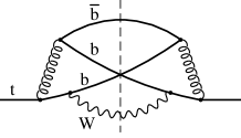
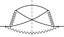
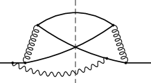
Figure 1: Non-planar diagrams contributing to the decay channel $t\to Wbb\bar{b}$.

In order to compute them, we expand around the point $m_{b}=m_{t}/3$. The expansion variable is $\tilde{\delta}$ such that

$$m_{b}=\frac{m_{t}}{3}\;(1-\tilde{\delta}).$$ (2)

We introduce the following notations: $p_{1,2}$ the momenta of the virtual gluons which later split into $b\bar{b}$ pairs, namely: $p_{1}=p_{4}+p_{5}$ and $p_{2}=p_{3}+p_{4}$. $p_{3},p_{5}$ are the $b$ quark momenta and $p_{4}$ is the antiquark momentum in the final state. $W$ denotes the $W$-boson momentum, $t$ is the top quark momentum. $p_{7}$ and $p_{6}$ are the momenta of the virtual top propagators: $p_{6}=t-p_{1}$ and $p_{7}=t-p_{2}$. $b$ is the momentum of the virtual $b$–quark, $b=t-W$.

All propagators can be expanded around the static limit, because the configuration around which we expand is the top quark decaying into three $b$–quarks at rest. For instance, the leading term in the expansion of the gluon propagator $1/p_{1}^{2}$ is $1/(4m_{b}^{2})$. The virtual top propagators give:

$$\frac{1}{(t-p_{1})^{2}-m_{t}^{2}}\to-\frac{1}{4m_{b}(m_{t}-m_{b})},$$ (3)

etc. Therefore, no dependence on phase space variables remains in the expanded denominators and the integration over the phase space can be performed by successive factorization into two-particle phase spaces.

First we introduce the vector $H$ which combines $p_{4}$ and $p_{5}$: $H=p_{4}+p_{5}$. We decompose $p_{4,5}$ into components parallel and perpendicular (in four-dimensional sense) to the $H$ direction. After averaging over directions of the perpendicular components this phase space integration gives the volume factor

$$R_{2}(H;p_{4},p_{5})={\pi\over 2}\sqrt{1-{4m_{b}^{2}\over H^{2}}}.$$ (4)

Next, we combine $H$ and $W$ into $Q=H+W$. Since $W$ is masseless, this phase space gives no square root function

$$R_{2}(Q;H,W)={\pi\over 2}{Q^{2}-H^{2}\over Q^{2}}.$$ (5)

We are then left with $t=Q+p_{3}$ phase space and two integrations over $H^{2}$ and $Q^{2}$. The integration limits are $4m^{2}<Q^{2}<(M-m)^{2}$ and $4m^{2}<H^{2}<Q^{2}$. Also, the $Q,p_{3}$ phase-space is given by Källén function, the momentum of the $Q$ in the rest frame of $t$:

$$R_{2}(t;Q,p_{3})={\pi\over 2m_{t}^{2}}\sqrt{[(m_{t}-m_{b})^{2}-Q^{2}][(m_{t}+m_{b})^{2}-Q^{2}]}.$$ (6)

Finally, for $H^{2}$ and $Q^{2}$ we introduce variables $x_{1,2}\in(0,1)$, defined by $H^{2}=4m^{2}(1+\omega x_{1}x_{2})$ and $Q^{2}=4m^{2}(1+\omega x_{1})$. From the limits on $H^{2}$ and $Q^{2}$ we find

$$\omega={(m_{t}-m_{b})^{2}\over 4m_{b}^{2}}-1\sim\tilde{\delta}$$ (7)

and the volume of the phase space $R_{2}(t;Q,p_{3})$ is given by

$$R_{2}(t;Q,p_{3})={4m_{b}\over\sqrt{3}m_{t}}\sqrt{\omega}\sqrt{1-x_{1}}\sqrt{1-{{\tilde{\delta}}^{2}\over 4}-{x_{1}\tilde{\delta}\over 4}(4-\tilde{\delta})},$$ (8)

where the last square root can be expanded in $\tilde{\delta}$. Also the $\sqrt{1-4m^{2}/H^{2}}$ expressed in terms of $x_{1,2}$ becomes proportional to $\sqrt{x_{1}x_{2}}$. As a result we obtain an expression containing only half-integer or integer powers of $x_{1,2}$ which can be easily integrated.

3 Two-loop corrections to top decay rate

In the limit of vanishing $W$ mass, the width of the decay $t\to bW$ is given by the formula (we neglect terms ${\cal O}(\alpha_{s}^{3})$)

$$\Gamma(t\to bW)=\Gamma_{0}\left[a_{0}+\frac{\alpha_{s}(m_{t})}{\pi}C_{F}a_{1}+\left(\frac{\alpha_{s}}{\pi}\right)^{2}C_{F}a_{2}\right],$$ (9)

where $\Gamma_{0}=\frac{G_{F}m_{t}^{3}}{8\sqrt{2}\pi}|V_{tb}|^{2}$. In this paper we use $\alpha_{s}(m_{t})$ determined in the $\overline{\rm MS}$ scheme and $m_{t,b}$ are the pole masses. $a_{0}=(1-m_{b}^{2}/m_{t}^{2})^{3}$ and $a_{1}$ is also known in a closed analytical form [13, 22]. In the limit of the vanishing $b$ quark mass we have

$$a_{0}=1,\qquad a_{1}={5\over 4}-{\pi^{2}\over 3}.$$ (10)

$a_{2}$ is the main new result of the present paper. It can be divided up into 4 gauge invariant parts

$$a_{2}=\left(C_{F}-{C_{A}\over 2}\right)a_{F}+C_{A}a_{A}+T_{R}N_{L}a_{L}+T_{R}a_{H},$$ (11)

where $C_{F}=4/3$, $C_{A}=3$, $T_{R}=1/2$, and $N_{L}$ is the number of quark flavors whose masses can be neglected. For the top quark decay we take $N_{L}=5$. $a_{F,A,L,H}$ are functions of the mass ratio of the $b$ and $t$ quarks. We have calculated them using an expansion around the equal mass case. The expansion parameter, $\delta\equiv 1-m_{b}/m_{t}$ is close to one, so that many terms of the series must be calculated in order to obtain good accuracy. Such expansion has already been considered in our previous work [23, 21]. In those papers we have defined the quantities $\Delta_{F,A,L,H}$. Two coefficient functions in eq. (11), $a_{A,L}$, coincide with $\delta^{3}\Delta_{A,L}$. For the purpose of the present application we have more than doubled the number of terms in the expansion. $a_{H}$ is analogous to $\delta^{3}\Delta_{H}$, except that it now contains contributions of the top quark loop only. The $b$ quark loop and part of real $b\bar{b}$ pair radiation is accounted for by adjusting $N_{L}$. There is, however, part of real $b\bar{b}$ pair production which cannot be described in this way. It corresponds to the non-planar interference diagrams shown in fig. 1 and is included in $a_{F}$, which without these diagrams would have coincided with $\delta^{3}\Delta_{F}$. These diagrams, contributing to the decay $t\to Wbb\bar{b}$, have no analogs in the $b-c$ transitions considered in [23, 21].

For $m_{b}\to 0$, $a_{L}$ was obtained numerically in [16], and is now known analytically in this limit [17]:

$$a_{L}(m_{b}=0)=-{4\over 9}+{23\over 108}\pi^{2}+\zeta_{3},\qquad\zeta_{3}\simeq 1.2020569.$$ (12)

The dependence of the coefficient functions $a_{i}$ on $m_{b}/m_{t}$ is shown in fig. 2. For $m_{b}/m_{t}\approx 4.8/175$ we find the following numerical values:

$$\mbox{For }m_{b}/m_{t} = 4.8/175:$$

$$a_{F} = 3.4(2),\qquad a_{A}=-6.28(2),\qquad$$

$$a_{L} = 2.83(4),\qquad a_{H}=-0.06349(1).$$ (13)

We note that $a_{F}$ has the largest error bar. This is because there are two separate series contributing to it: in addition to the series in $\delta=1-m_{b}/m_{t}$ there is also the non-planar contribution expanded in $\tilde{\delta}=1-3m_{b}/m_{t}$. Both these series are separately divergent in the limit $m_{b}\to 0$ like $\ln^{3}(m_{b})$. For this reason their reliable estimate near this limit is difficult and we have assigned a conservative error bar to the result. On the other hand, because of the color factors in eq.(11), the final result for $a_{2}$ is not very sensitive to the relatively large error in $a_{F}$.

The expressions we have obtained for $a_{F,A,L}$ contain the first and second powers of $\ln(2\delta)$. It turns out that the convergence of these series is improved if we rewrite these terms as $\ln(2\delta)=\ln\beta-\ln(1-\delta/2)$, with $\beta=\delta(2-\delta)$ and expand $\ln(1-\delta/2)$ in $\delta$. Since $\beta$ approaches 1 much faster than $\delta$, the remaining logs are smaller. Because of the many terms which had to be evaluated for the coefficient functions $a_{i}$, the results are rather lengthy and not suitable for publication in a journal. However, they can be obtained from the authors upon request.

In the future, it is likely that the corrections to $t\to bW$ will be calculated analytically in the point $m_{b}=0$. We therefore list here our estimates for the numerical values of $a_{i}$ in this point:

$$\mbox{For }m_{b}/m_{t} = 0:$$

$$a_{F} = 3.5(2),\qquad a_{A}=-6.35(7),\qquad$$

$$a_{L} = 2.85(7),\qquad a_{H}=-0.06360(1).$$ (14)

The value of $a_{L}$ found from our expansion is in agreement with the exact value obtained from eq. (12), $a_{L}(m_{b}=0)=2.859473\ldots$.

       (a)        (b)        (c)        (d)

Figure 2: Plots of the coefficient functions defined in eq. (11): (a) $a_{F}$, (b) $a_{A}$, (c) $a_{L}$, (d) $a_{H}$. The variable on the horizontal axis is $m_{b}/m_{t}$.

Let us now discuss the numerical value of the correction in the case of the massless $b$ quark. For the purpose of discussion it is convenient to separate the BLM [15] and the non-BLM corrections to the decay rate. The BLM corrections follow immediately from the results of [16, 17] and in present notations are given by:

$$a_{2}^{\rm BLM}=-T_{R}\left(\frac{33}{2}-N_{L}\right)a_{L}.$$ (15)

Using $N_{L}=5$, we obtain:

$$a_{2}^{\rm BLM}(m_{b}=0)=-16.442\ldots.$$ (16)

This is to be compared with the complete result for $a_{2}$,

$$a_{2}(m_{b}=0)=-12.5(4).$$ (17)

The complete ${\cal O}(\alpha_{s}^{2})$ corrections are smaller by 24% than the BLM estimate. This difference is somewhat larger than in $b\to c$ decays [23, 21].

In any case, numerically the second order corrections appear to be very moderate:

$$\Gamma_{t}(m_{b}/m_{t}=0)=\Gamma_{0}\left(1-0.866\;\alpha_{s}(m_{t})-1.69(5)\;\alpha_{s}^{2}\right).$$ (18)

For $m_{b}/m_{t}=4.8/175$ we find

$$a_{2}(m_{b}/m_{t}=4.8/175) = -12.4(3),\qquad a_{2}^{\rm BLM}(m_{b}/m_{t}=4.8/175)=-16.3(2);$$

$$\Gamma_{t}(m_{b}/m_{t}=4.8/175) = 0.998\times\Gamma_{0}\left(1-0.857\alpha_{s}(m_{t})-1.68(4)\alpha_{s}^{2}\right).$$ (19)

Using $\alpha_{s}(m_{t})=0.11$, we find that the ${\cal O}(\alpha_{s}^{2})$ corrections to the top decay width are very close to 2%.

Finally, we list here also the values obtained for $\delta=0.7$, or $m_{b}/m_{t}=0.3$, which after replacement $t,b\to b,c$ are relevant for the differential width of $b\to c+\mbox{leptons}$, when the leptons are emitted parallel to each other, i.e. with a zero invariant mass:

$$\mbox{For }m_{b}/m_{t} = 0.3:$$

$$a_{F} = 1.37261(2),\qquad a_{A}=-3.09498(4),\qquad$$

$$a_{L} = 1.31091(5),\qquad a_{H}=-0.05061395(1).$$ (20)

At $m_{b}/m_{t}=0.3$ one has to account for the finite $b$ mass in the virtual loop. This amounts to replacing $a_{H}$ by $\tilde{a}_{H}$, which corresponds to $\delta^{3}\Delta_{H}$ in [23, 21]. At $\delta=1-m_{b}/m_{t}=0.7$ we find

$$\tilde{a}_{H}=a_{H}+(b\mbox{-loop})\simeq-0.0506+0.6333=0.5827.$$ (21)

4 Conclusion

We have presented a calculation of the ${\cal O}(\alpha_{s}^{2})$ corrections to the decay width of the top quark $\Gamma(t\to bW)$ in the limit $m_{t}\gg m_{W}$. For $\alpha_{s}(m_{t})=0.11$, we found (see eqs. (18, 19)) that the second order QCD corrections decrease the value of the top width by 2%.

To perform this calculation, we used the methods described in detail in [21]. Also, since the process $t\to b\bar{b}bW$ contributes to the top decay width at order ${\cal O}(\alpha_{s}^{2})$, we had to develop a new technique to deal with the “non-planar” interference diagrams.

The decay rate of the top quark is proportional to the third power of its mass. In our calculations we used the pole mass of the top quark. It has been demonstrated [18] that the convergence of the perturbation series is improved if one parametrizes the width formula in terms of the $\overline{\rm MS}$ mass. We have not performed this reparametrization here, since the second order corrections are small even if the pole mass is used. We note, however, that employing the $\overline{\rm MS}$ mass is likely to decrease them even further.

With the electroweak corrections and effects of the $W$ width on $\Gamma_{t}$ known, our result provides the last missing ingredient in predicting the top decay width in the SM with accuracy $\sim 1\%$. The remaining uncertainty is presently dominated by the top quark mass. It is difficult to say at the moment whether or not the experimental determination of the top quark width can be performed with a comparable precision. A future muon collider might be the best place for such measurements.

References

- [1] J. H. Kühn, Acta Phys. Pol. B12, 347 (1981).
- [2] E. Accomando et al. (ECFA/DESY LC Physics Working Group), Phys. Rep. 299, 1 (1998).
- [3] M. Jeżabek, Nucl. Phys. Proc. Suppl. 37B, 197 (1994).
- [4] A. H. Hoang and T. Teubner, hep-ph/9801397.
- [5] K. Melnikov and A. Yelkhovsky, hep-ph/9802379, in press in Nucl. Phys. B.
- [6] M. Peter, Phys. Rev. Lett. 78, 602 (1997); Nucl. Phys. B501, 471 (1997).
- [7] M. Jeżabek et al., hep-ph/9802373, in press in Phys. Rev. D.
- [8] K. Fujii, cited in [10].
- [9] J. H. Kühn, in The top quark and the electroweak interaction, edited by J. Chan and L. DePorcel (SLAC, Stanford, 1997), p. 1, Proc. of the 23rd SLAC Summer Institute.
- [10] M. Jeżabek and J. H. Kühn, Phys. Rev. D48, 1910 (1993), e: ibid. D49, 4970 (1994).
-
[11]
N. Cabibbo and L. Maiani, Phys. Lett. B79, 109 (1978).
A. Ali and E. Pietarinen, Nucl. Phys. B154, 519 (1979).
N. Cabibbo, C. Corbò, and L. Maiani, Nucl. Phys. B155, 93 (1979).
G. Altarelli et al., Nucl. Phys. B208, 365 (1982).
Q. Hokim and X.-Y. Pham, Ann. Phys. (N.Y.) 155, 202 (1984). -
[12]
R. E. Behrends, R. J. Finkelstein, and A. Sirlin, Phys. Rev. 101, 866
(1956).
S. Berman, Phys. Rev. 112, 267 (1958).
T. Kinoshita and A. Sirlin, Phys. Rev. 113, 1652 (1959). - [13] M. Jeżabek and J. H. Kühn, Nucl. Phys. B314, 1 (1989).
-
[14]
A. Czarnecki, Phys. Lett. B252, 467 (1990).
C. S. Li, R. J. Oakes, and T. C. Yuan, Phys. Rev. D43, 3759 (1991). - [15] S. J. Brodsky, G. P. Lepage, and P. B. Mackenzie, Phys. Rev. D28, 228 (1983).
- [16] B. H. Smith and M. B. Voloshin, Phys. Lett. B340, 176 (1994).
- [17] A. Czarnecki, Acta Phys. Pol. B26, 845 (1995).
- [18] M. Beneke and V. M. Braun, Phys. Lett. B348, 0513 (1995).
- [19] T. Mehen, Phys. Lett. B417, 353 (1998); B382, 267 (1996).
-
[20]
A. Denner and T. Sack, Nucl. Phys. 358, 46 (1991).
G. Eilam, R. Mendel, R. Migneron, and A. Soni, Phys. Rev. Lett. 66, 3105 (1991). - [21] A. Czarnecki and K. Melnikov, Phys. Rev. D 56, 7216 (1997).
- [22] A. Czarnecki and S. Davidson, Phys. Rev. D 48, 4183 (1993).
- [23] A. Czarnecki and K. Melnikov, Phys. Rev. Lett. 78, 3630 (1997).