Factorization is not violated

Abstract

We show that existing proofs of factorization imply the cancellation of certain multiladder contributions that Gotsman, Levin, and Maor had suggested would invalidate the basic factorization theorem in QCD. No modifications of the original argument are necessary, although the details of the example offer useful insight into the mechanisms of factorization.

1 Introduction

Factorization theorems are at the heart of the theory of high-energy inclusive processes involving a large momentum transfer. Examples include the inclusive production in hadron-hadron collisions of new, heavy particles, such as the Higgs boson or the supersymmetric partners of the currently known particles. These theorems apply to inclusive cross sections for the production of a set $F$ of heavy particles or of a system of jets with a total mass $Q$,

$$A+B\rightarrow F(Q)+X\,.$$ (1)

The theorem assumes that $F$ is defined in such a way that all final states that differ by the emission of soft hadrons and by the collinear rearrangement of momenta between outgoing light hadrons are summed over. It is important here that $Q$ be large. One usually assumes that $Q$ is of the order of the $AB$ invariant mass $\sqrt{s}$. For $1\ {\rm GeV}\ll Q\ll\sqrt{s}$, one should sum logarithms of $\sqrt{s}/Q$ to improve the usefulness of the perturbative expansion used in the calculations.

According to the factorization theorem, the cross section for (1) may be written as a convolution of parton distributions and perturbative hard scattering functions,

$$\sigma_{AB}=\sum_{ab}\int dx_{a}dx_{b}\,\phi_{a/A}(x_{a},\mu^{2})\,\phi_{b/B}(x_{b},\mu^{2})\,\hat{\sigma}_{ab}\!\left({Q^{2}\over x_{a}x_{b}s},{Q\over\mu},\alpha_{s}(\mu)\right)\,\left(1+{\cal O}\left({1\over Q^{P}}\right)\right)\,.$$ (2)

Here, the nonperturbative functions $\phi_{c/C}(x_{c},\mu^{2})$ give the distribution of parton $c$ in hadron $C$ as a function of the longitudinal momentum fraction $x_{c}$, evolved to factorization scale $\mu$. The hard-scattering function $\hat{\sigma}_{ab}$ is computed in perturbation theory up to some order, $\alpha_{s}^{N}$, leaving corrections of order $\alpha_{s}^{N+1}$. As indicated, corrections to the factorization formula are suppressed by a positive power, $P$, of the large mass.

Despite their central role, the foundations of the factorization theorems have received rather little theoretical attention in recent years beyond the arguments given in Ref. [1, 2] and reviewed in Ref. [3]. An exception is a recent paper by Gotsman, Levin, and Maor [4], which discusses the possibility of corrections to the right-hand side of Eq. (2) that are not power-suppressed at all. These conjectured corrections are associated with the exchange of ladders of the reggeon type. It is our aim in this paper to show that such exchanges do not require a revision of Eq. (2), and that, indeed, in an inclusive cross section of the type described above, contributions from the regions of momentum space identified in [4] cancel. We shall rely heavily on the discussion of Ref. [2], and will not find it necessary to modify the reasoning presented there. Indeed, the discussion of that paper already includes the treatment of the effect identified in Ref. [4], to all orders in perturbation theory. Nevertheless, since Ref. [2] does not include low-order examples, the treatment of a rapidity-ordered ladder will, we hope, illustrate and perhaps clarify the proof.

2 Ladder Diagrams in Inclusive Cross Sections

We consider the cross section $d\sigma/dy$ for the production of a Higgs boson with rapidity $y$ in the collision of two hadrons with c.m. energy $\sqrt{s}$. Our hadrons each consist of a simple quark-antiquark pair with a pointlike coupling to the hadron field. The hard scale in the problem is the Higgs boson mass, which we denote by $Q$. We may have $s\sim Q^{2}$ or $s\gg Q^{2}$. Our analysis works in either case.

We analyze cut Feynman diagrams for Higgs boson production that arise from the uncut graph shown in Fig. 1. This choice of graph is motivated by the suggestion of Gotsman et al. [4], who examine graphs similar to this. This graph contains enough of the physics to be instructive, while it is of low enough order to be treated in detail. We hope that it will be evident that the argument given below for the graph of Fig. 1 could be applied to more complicated graphs.

In Fig. 1, the star represents the hard scattering matrix element for ${\rm gluon}+{\rm gluon}\to{\rm Higgs\ boson}$. The lowest order diagram for this, containing a top quark loop, is shown in Fig. 2. We shall treat only the case where Higgs production appears on the “outer” sides of the ladders, as in Fig. 1. Moving the starred vertex to the other side of either or both ladders [4] leads to diagrams that can be treated by exactly the same methods as Fig. 1.

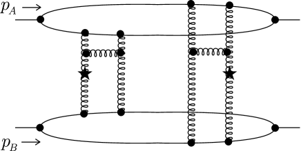
Figure 1: The uncut version of the graph analyzed in this paper.

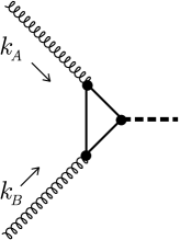
Figure 2: The hard subgraph, represented by a star in our graphs.

We take $p^{\mu}_{A}=\left(p^{+}_{A},0,{\bf 0}\right)$ and $p^{\mu}_{B}=\left(0,p^{-}_{B},{\bf 0}\right)$, where $p^{\pm}=(p^{0}\pm p^{3})/\sqrt{2}$. Then $2p_{A}^{+}p_{B}^{-}=s$. Let the Higgs boson momentum be $q^{\mu}$, so $q_{\mu}q^{\mu}=Q^{2}$. It is helpful to have a specific reference frame in mind. Let us choose the reference frame in which $q^{+}=q^{-}$.

There are various integration regions that make leading contributions to the cross section. We consider the region in which all transverse momenta are of order $m$ ($m\sim 1\ {\rm GeV}\ll Q$) and in which all lines outside the hard scattering have virtuality at most of order $m^{2}$. We take quark masses to be of order $m$. The gluons entering the hard interaction have momenta $k^{\mu}_{A}=\left(k^{+}_{A},k^{-}_{A},{\bf k}_{A}\right)$, $k^{\mu}_{B}=\left(k^{+}_{B},k^{-}_{B},{\bf k}_{B}\right)$ where $k_{A}^{+}$ and $k_{B}^{-}$ are of order $Q$. The transverse components ${\bf k}_{A}^{\mu}$ and ${\bf k}_{B}^{\mu}$ are of order $m$. Then $k_{A}^{-}$ and $k_{B}^{+}$ are much smaller than $m$, of order $m^{2}/Q$ in order that $k_{A}^{2}\sim k_{B}^{2}\sim m^{2}$. In the integration region of interest, all of the lines in the upper part of the graph carry large $+$ momenta, with positive $+$ momentum carried from left to right through the graph. The transverse momentum components are all of order $m$ and the $-$ components are all small. Now consider the bottom part of the graph, not including the two gluons exchanged between top and bottom. All of the of the lines here carry large $-$ momenta, with positive $-$ momentum carried from left to right through the graph. The transverse momentum components are all of order $m$ and the $+$ components are all small. We shall refer to this as the “ladder region” of momentum space.

There are two one-rung ladders in the diagram. For the left hand ladder, for instance, we choose the labeling shown in Fig. 3. As mentioned above, we work in the integration region with $\ell_{A}^{T}\sim k_{A}^{T}\sim q_{1}^{T}\sim m$. We take $k^{+}_{A}=x\,p^{+}_{A}$ and $\ell^{+}_{A}=z\,p^{+}_{A}$ with $x_{A}<z<1$. If $x_{A}\ll 1$ then $z$-integration over this range can give a large logarithm $\ln(1/x_{A})$, where the logarithm comes from the strongly ordered region $x_{A}\ll z\ll 1$. However, we do not need strong ordering. What is important for us is that $\ell_{A}^{+}$, $k_{A}^{+}$ and $\ell_{A}^{+}-k_{A}^{+}$ are large and positive, at least of order $Q$.

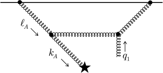
Figure 3: Labeling of momenta for one of the ladder subdiagrams.

By assumption, we are in a region of momentum where the exchanged gluon with momentum $q_{1}^{\mu}$ has $q_{1}^{T}\sim m$ and all the lines outside the hard scattering have virtuality at most of order $m^{2}$. Then the important integration region for $q_{1}^{+}$ is $|q_{1}^{+}|\,\lower 3.0pt\hbox{\vbox{\hbox{$<$} \kern-9.0pt\hbox{$\sim$}}}\,m^{2}/Q$ so that propagators in the $B$ system are not far off shell. Similarly, the important integration region for $q_{1}^{-}$ is $|q_{1}^{-}|\,\lower 3.0pt\hbox{\vbox{\hbox{$<$} \kern-9.0pt\hbox{$\sim$}}}\,m^{2}/Q$. Then $\left|q_{1}^{+}q_{1}^{-}\right|\,\lower 3.0pt\hbox{\vbox{\hbox{$<$} \kern-9.0pt\hbox{$\sim$}}}\,m^{4}/Q^{2}\ll m^{2}\sim q^{2}_{T}$, so we can simplify our problem by replacing

$$q_{1\mu}q_{1}^{\mu}=2q_{1}^{+}q_{1}^{-}-q_{1T}^{2}\rightarrow-q^{2}_{1T}$$ (3)

in the gluon propagator. With this replacement for $q_{1}$, the soft gluon line has $q_{1}^{\mu}q_{1\mu}<0$, so that it can never cross the final state cut. (This is just to reduce the number of cuts considered. Our standard analysis [2] does not use this assumption, which allows us to consider also $|q_{1T}^{2}|\ll m^{2}$.) Exactly similar remarks apply to the soft gluon, of momentum $q_{2}$, in the other ladder.

Now, following the argument in Ref. [2], we break up our graph into $J_{A}$ and $R$, as shown in Fig. 4. The jet subgraph $J_{A}$ contains all of the lines near the mass shell with large plus momenta, $k^{+}\,\lower 3.0pt\hbox{\vbox{\hbox{$>$} \kern-9.0pt\hbox{$\sim$}}}\,Q$. The remaining subdiagram contains all of the other lines, including another jet subgraph with lines with large minus momenta, the two soft lines carrying momenta $q_{1}^{\mu}$ and $q_{2}^{\mu}$, and the hard subgraph.

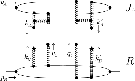
Figure 4: The basic diagram split into subdiagrams $J_{A}$ and $R$ corresponding to our chosen region of the loop momenta.

3 Cancellation of the Ladder Region

We now show the cancellation of the ladder region in the sum over cuts of Fig. 1. We proceed in a number of steps that follow the arguments of Ref. [2]. These start with some approximations that give power-suppressed errors.

Step 1. Neglect $k^{+}_{B}$ and $k_{B}^{\prime+}$ in $J_{A}$ so that subgraph $R$ includes $\int dk_{B}^{+}dk_{B}^{\prime+}$. Similarly, neglect $k_{A}^{-}$ and $k_{A}^{\prime-}$in $R$ so that subgraph $J_{A}$ includes $\int dk_{A}^{-}dk_{A}^{\prime-}$.

Step 2. Neglect $q_{1}^{+}$ and $q_{2}^{+}$ in $J_{A}$. This gives $\bar{R}=\int dq_{1}^{+}dq_{2}^{+}\ R\ \delta(k_{A}^{+}+{k^{\prime}_{A}}^{+}+q_{1}^{+}+q_{2}^{+})$. Also take $J_{A}^{\mu_{1}\mu_{2}}\ R_{\mu_{1}\mu_{2}}\rightarrow J_{A}^{++}R_{++}$.

Step 3. Show that $\bar{R}$ is independent of which side of the final state cut the upper ends of the two soft gluons are on.

Steps 4 and 5 will be explained later and illustrated by explicit calculation. Before proceeding to them, we need to discuss Step 3 in detail, since it is not obviously correct. We need to show that the four cuts of $R$ shown in Fig. 5 give equal contributions to $R$.

 

 

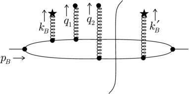
Figure 5: The four cuts of subgraph $R$.

In Ref. [2], we show this by writing the diagrams in $x^{-}$ ordered perturbation theory. Here we have an especially simple situation, so we can simplify the argument. Consider, for example, the first graph in Fig. 5.

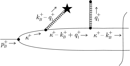
Figure 6: Routing of plus momentum for first cut of $R$

We can route $q_{1}^{+}$ and $q_{2}^{+}$ differently in different graphs because we are integrating over $k^{+}_{B}$ and we can shift the origin of the $k^{+}_{B}$ integration. In this particular graph, we choose to route $q_{1}^{+}$ directly to the left hand hard interaction, as illustrated in Fig. 6.

With this momentum routing, we perform the $q_{1}^{+}$ integration first. After accounting for the replacement (3), we see that there are two poles in the complex $q_{1}^{+}$ plane, one from the quark line carrying momentum $\kappa^{+}-k_{B}^{+}+q_{1}^{+}$ and one from the gluon line carrying momentum $k_{B}^{+}-q_{1}^{+}$. In the ladder region of integration, the quark lines in the figure all carry positive momentum fractions $\ell^{-}/p_{B}^{-}$ from left to right. Then the two poles in the $q_{1}^{+}$ plane are on opposite sides of the real $q_{1}^{+}$ axis. We close the $q_{1}^{+}$ integration contour in the lower half plane to put the quark line on shell. The result is the same as that obtained by replacing

$${i\over k^{2}-m^{2}+i\epsilon}\to 2\pi\,\delta(k^{2}-m^{2}),$$ (4)

just as if the quark were crossing a final state cut.

We make a similar choice for the $q_{2}^{+}$ integration. The result is shown in the first graph in Fig. 7, where we indicate the factors $\delta(k^{2}-m^{2})$ with “cut” symbols.

 

 

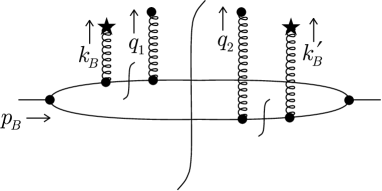
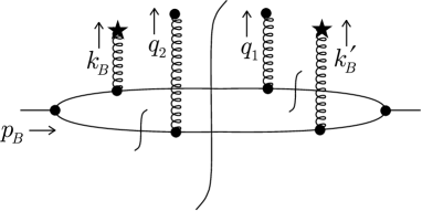
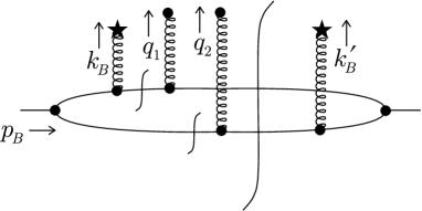
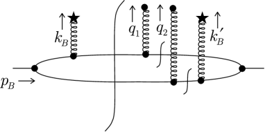
Figure 7: The four cuts of subgraph $R$ after performing the $q_{1}^{+}$ and $q_{2}^{+}$ integrations.

Now we do this for each of the four graphs. We get the results shown in Fig. 7. Evidently, all four of these cut graphs are equal, except for the factors of $i$ associated with the vertices and the uncut propagators. But to go from one graph to another we transfer one or more uncut propagators and the same number of vertices from one side of the final-state cut to the other. Hence the different cuts are in fact equal. QED.

Step 4. Now we look at $J_{A}$. In Ref. [2] we argue that, after summing over cuts, we can replace $q_{1}^{T}\to 0$ and $q_{2}^{T}\to 0$ in $J_{A}$. This involves showing (by writing the diagrams in $x^{-}$ ordered perturbation theory) that

a) after summing over cuts, poles in $q_{1}^{-}$ and $q_{2}^{-}$ near the origin are in the lower half planes;

b) we can deform the $q_{i}^{-}$ integration contours far into the upper half planes;

c) on the deformed contours, if $\ell^{\mu}$ is the momentum of a propagator through which $q_{i}^{\mu}$ flows, then $\ell^{-}$ becomes large: $\ell^{+}\ell^{-}\gg\ell_{T}^{2}$; thus we can set $q_{i}^{T}\to 0$;

d) finally, we can return the contours to the real axes.

Step 5. The argument in Ref. [2] proceeds to combine the results from different Feynman graphs, using gauge invariance, to finally write the result in a factored form.

In the present case we have an especially simple situation, so we can simplify the argument. In fact, the contribution from the ladder region to the graph we are considering vanishes at leading order in $1/Q$ by itself. Thus we do not need Step 5. We will therefore make a straightforward analysis of the graphs to show that

Step 4${\,}^{\prime}$. After summing over cuts, $J_{A}={\cal O}(1/Q)$ in the ladder region.

Since subgraph $R$ is the same no matter where we draw the cut, this implies that the sum over cuts of the original graph vanishes at the leading power of $1/Q$.

We now show explicitly that the sum over cuts of the jet subgraph $J_{A}$ gives zero. There are nine cuts of $J_{A}$ to consider. We look first at the three cuts shown in Fig. 8. Call these cut graphs $A$, $B$, and $C$. We have oriented the lines to indicate the direction of flow of the $+$ component of momentum; recall that the $+$ components of $q_{1}$ and $q_{2}$ have been set to zero in $J_{A}$.

 

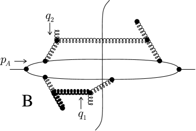
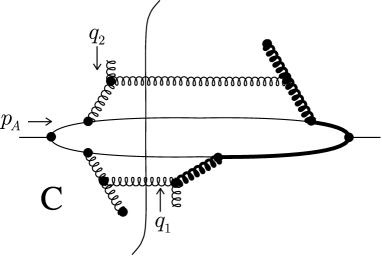
Figure 8: Three cuts of subgraph $J_{A}$.

We consider first cut graph $A$. This cut graph has a virtual loop, shown in more detail in Fig. 9. Let loop momentum $\ell^{-}$ circulate around this loop as shown in the first part of Fig. 9. Since, in the ladder integration region, positive $+$ momentum flows from left to right through the propagators in the figure, there are three poles in the upper half $\ell^{-}$ plane and one in the lower half $\ell^{-}$ plane. We close the contour in the lower half $\ell^{-}$ plane. This amounts to putting the quark line on shell, as indicated by the cut symbol in second part of Fig. 9. Next, we route $q_{1}^{-}$ to the hard vertex through the two gluon propagators, as depicted in the second part of Fig. 9. There are two poles in the $q_{1}^{-}$ plane. We perform the $q_{1}^{-}$ integral by closing the contour in the upper half plane, which amounts to putting the first gluon through which $q_{1}^{-}$ flows on shell. The result is indicated in the first graph, $A$, of Fig. 10.

    

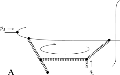
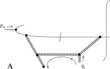
Figure 9: Treatment of cut A of $J_{A}$.

In cut graph $B$, we route $q_{1}^{-}$ to the hard vertex through the two gluon propagators, indicated by heavy lines in Fig. 8. Then closing the $q_{1}^{-}$ contour in the upper half plane gives the result indicated in the second graph, $B$, of Fig. 10

In cut graph $C$, we route $q_{1}^{-}$ to the hard vertex to the right, through a gluon propagator, two quark propagators, and two more gluon propagators, indicated with heavy lines. There are five poles in the $q_{1}^{-}$ plane, two in the upper half plane and three in the lower half plane. We perform the $q_{1}^{-}$ integral by closing the contour in the upper half plane. Then there are two terms. The two terms are indicated in the third and fourth graphs, $C1$ and $C2$, of Fig. 10.

Now we note that $C1$ cancels $A$, while $C2$ cancels $B$: in each of the canceling pairs of graphs, the propagators and vertices are the same up to sign and there are an odd number of sign changes resulting from moving uncut propagators and vertices from one side of the final state cut to the other.

 

 

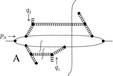
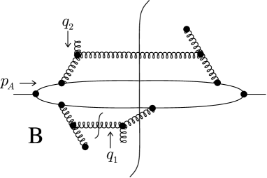
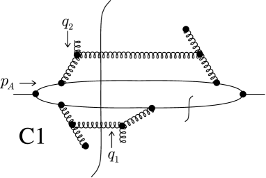
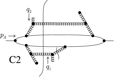
Figure 10: Three cuts of subgraph $J_{A}$ after performing minus integrations.

There are more cut graphs. For each way that we cut the right hand ladder, there are three ways to cut the left hand ladder. Thus we could label the graphs $G(n,m)$ with $n=A,B,C$ denoting the cut for the left hand ladder and $m=A,B,C$ denoting the cut for the right hand ladder. In this notation, what we have seen is that $G(A,C)+G(B,C)+G(C,C)={\cal O}(1/Q)$. The same argument shows that

$$\sum_{n=A,B,C}G(n,m)={\cal O}(1/Q)\quad m=A,B,C.$$ (5)

A similar argument also shows that

$$\sum_{m=A,B,C}G(n,m)={\cal O}(1/Q)\quad n=A,B,C.$$ (6)

Thus there is a double cancellation.

We conclude that the sum over all cuts of Fig. 1 is ${\cal O}(1/Q)$ and we do not have a violation of factorization.

4 Extensions of the argument

Gotsman et al. consider more elaborate diagrams than the diagram of Fig. 1 that we have analyzed here. For instance, they consider exchanges of gluon ladders with arbitrary numbers of rungs. In addition, they concentrate on the region of integration space in which the rapidities of the rungs are strongly ordered. It should be evident that the calculation given above could be applied to more complicated diagrams. There would be little to change in the pattern of cancellation found here, which illustrates the general argument of Ref. [1, 2], although the notation would have to be more complicated. We draw attention to the fact that although factorization applies in the strongly ordered region that gives the leading small $x$ logarithms, factorization also applies in other regions: strong ordering of rapidities is not essential to the argument.

The argument presented here applies when the exchanged gluons have transverse momentum of order $m$, and when none of the lines outside of the hard scattering has virtuality much larger than $m^{2}$. This is also the region discussed in Ref. [4]. Other regions than the one we considered here are correctly treated by other parts of the factorization proof in [1, 2].

Let us close with a few additional comments relating our work to that of Ref. [4]. Gotsman et al. use modified AGK cutting rules to perform their calculation, finding a remainder after summing over final states. Such an analysis, however, assumes that the incoming particles to which the ladders attach are on-shell. In addition, we believe that this analysis is exact only at the level of leading logarithms. However, their noncancelling result (Eq. (8) in Ref. [4]), which is proportional to the square of the real part of their single-ladder exchange amplitude, is suppressed by two logarithms compared to leading logarithms.

We may note two specific differences between our analysis and that of Gotsman et al., both of which are important beyond the leading logarithmic approximation. First, they ignore certain final-state cuts, for example cut B in Fig. 8. This cut crosses the side of a ladder. Such a cut is not allowed in the leading logarithm approximation, but it is present when one goes beyond leading logarithms. Observe that the cut in question would not be kinematically allowed if the gluon ladder coupled to on-shell quark lines instead of internal off-shell lines. Second, Gotsman et al. appear to have ignored the loop integral that we label $k_{B}^{+}$, which we use to prove that the subgraph $R$ is independent of the final state cut of $J_{A}$ (Step 3). Both the extra cuts and the integral over $k_{B}^{+}$ are necessary to evaluate the ladder region fully. The proof of factorization that we gave in Ref. [1, 2] applies to the full leading-power contribution and not just to leading logarithms. It is this more general method that we have explained in the context of particular Feynman graphs.

Although we believe that factorization works, we should emphasize our concern that improvements are needed in the rigor of existing proofs of factorization [2, 3]. Conspicuously lacking are iterative algorithms for demonstrating (2) along the lines of those available for proofs of renormalization. Our presentation here is not a step in this direction, rather it is an illustration of already-existing arguments. We believe, however, that it is possible to construct such an algorithm (Cf. Ref. [5]). Improvements in the proof would help both to increase confidence in factorization and to clarify its variant applications, for instance to transverse momentum distributions [6] in the range of $Q_{T}\ll M$. We therefore welcome the motivation provided by [4] to reopen the discussion of these important issues.

References

- [1] J.C. Collins, D.E. Soper and G. Sterman, Nucl. Phys. B 261 (1985) 104; G.T. Bodwin, Phys. Rev. D 31 (1985) 2616, E. D 34 (1986) 3932.
- [2] J.C. Collins, D.E. Soper and G. Sterman, Nucl. Phys. B 308 (1988) 833.
- [3] J.C. Collins, D.E. Soper and G. Sterman, in Perturbative QCD, edited by A. H. Mueller (World Scientific, Singapore, 1989).
- [4] E. Gotsman, E. Levin, and U. Maor, Phys. Lett. B 406 (1997) 89, e-Print Archive: hep-ph/9705205; E. Levin, in DIS 97, Proceedings of the 5th International Workshop on Deep Inelastic Scattering and QCD, edited by J. Repond and D. Krakauer, AIP Conf. Proc. 407, (AIP, New York, 1997), p. 970, e-Print Archive: hep-ph/9705375.
- [5] J.C. Collins and D.E. Soper, Nucl. Phys. B 193 (1981) 381; F.V. Tkachov, e-Print Archive: hep-ph/9703432
- [6] J.C. Collins, D.E. Soper and G. Sterman, Nucl. Phys. B 250 (1985) 199; G. Altarelli, R.K. Ellis, M. Greco and G. Martinelli, Nucl. Phys. B 246 (1984) 12; C.T.H. Davies and W.J. Stirling, Nucl. Phys. B 244 (1984) 337 ; C.T.H. Davies, B.R. Webber and W.J. Stirling, Nucl. Phys. B 256 (1985) 413; P.B. Arnold and R.P. Kauffman, Nucl. Phys. B 349 (1991) 381; G.A. Ladinsky and C.P. Yuan, Phys. Rev. D 50 (1994) R4239, e-Print Archive: hep-ph/9311341.