IR-Renormalon Contributions to the
Structure Functions $g_{3}$ and $g_{5}$

Abstract

We calculate the leading $1/N_{f}$ perturbative contributions to the polarized nonsinglet structure functions $g_{3}$ and $g_{5}$ to all orders in $\alpha_{s}$. The contributions from the first renormalon pole are determined. It is a measure for the ambiguity of the perturbative calculation and is assumed to dominate the power corrections. The corrections $\Delta g_{3}$ and $\Delta g_{5}$ are given as functions of the Bjorken variable $x$ and turn out to be negligable. The anomalous dimensions of the leading twist operators are obtained in the next-to-leading order.

It is well known that the perturbation series for moments of twist-2 structure functions is an asymptotic one. This property can be studied in detail in the $1/N_{f}$-limit, in which the complete series can be calculated explicitely. Formally this series is given by an integral over the positive real axis in the Borel plane. This integral is ambiguous due to singularities on the integration path, the so called IR-renormalon poles. The residues of these poles are a measure for the ambiguity of the perturbative series. The so-called hypothesis of UV-dominance allows furthermore to interpret this ambiguity as an estimate for the power corrections. the program just sketched was already applied to all twist-2 structure functions except $g_{3}(x,Q^{2})$ and $g_{5}(x,Q^{2})$ [1] – [3]. In this contribution we investigate these remaining two cases. Good experimental data for power corrections to structure functions exists so far only for $F_{L}$. The renormalon prediction fits this data surprisingly well. Let us note that similar renormalon analyses have recently been applied to a large range of other QCD observables [4] – [11].

The Borel transformation of a perturbative series

$$R=r_{0}a+r_{1}a^{2}+r_{2}a^{3}=\ldots=\sum_{n=0}^{\infty}r_{n}a^{n+1}\;,\quad a=\alpha_{s}\cdot 4\pi$$ (1)

is defined as

$$B[R](u)=\sum_{n=0}^{\infty}u^{n}\frac{r_{n}}{n!}\;.$$ (2)

$R$ can be reobtained from its Borel transform by an integration over the positive real axis as

$$R=\int_{0}^{\infty}\mathrm{d}u\,\mathrm{e}^{-u/a}B[R](u)\;.$$ (3)

The coefficients of the original power series can also be obtained individually by taking the derivatives with respect to $u$

$$r_{k}=\frac{\mathrm{d}^{k}}{\mathrm{d}u^{k}}B[R](u)\Bigg{|}_{u=0}\;.$$ (4)

$B[R]$ has pole singularities on the real axis, the so-called renormalons [12]. The poles on the positive $u$-axis, which are called IR-renormalons because they can be traced back to low momentum contribution to the loop integrals, lead to ambiguities in the retransformation (3) because it is unclear wether they have to be passed above or below. The fact that no unambiguous retransformation exists reflects the fact that the perturbative expansions are asymptotic [13, 14]. The ambiguities are of the order of magnitude

$$\Delta R=\mathrm{e}^{-u/a}\mbox{Res}\Big{(}B[R](u)\Big{)}\Bigg{|}_{u=\mbox{\footnotesize pole position}}\;,$$ (5)

and can be interpreted as a measure for generic uncertainties of perturbative predictions or in other words as an estimation for corrections beyond leading twist perturbation theory [4].

In connection with the investigation of renormalons the NNA-approximation (naive non-Abelianization) [15] is of particular interest because in the Borel it leads plane to an effective gluon propagator of a very simple form allowing a calculation to all orders in the coupling constant. In the NNA-approximation we start with a restriction to the leading $1/N_{f}$-terms ($N_{f}$: number of quark flavors), which is the sum of all diagrams with only one exchanged gluon but an arbitrary number of quark loops. The missing terms are then approximated by the replacement $N_{f}\rightarrow-24\pi^{2}\beta_{0}=N_{f}-33/2$, which corresponds to a restriction to the leading terms of an expansion in the one loop $\beta$-function of QCD $\beta_{0}=\frac{1}{(4\pi)^{2}}(11-\frac{2}{3}N_{f})$. The resummation of all corresponding diagrams leads to the Borel transformed effective gluon propagator

$$B[g^{2}D_{\mu\nu}^{ab}(k)](s)=\delta^{ab}\frac{g_{\mu\nu}-\frac{k_{\mu}k_{\nu}}{k^{2}}}{k^{2}}\Bigg{(}\frac{\mu^{2}\mathrm{e}^{-c}}{-k^{2}}\Bigg{)}^{s}$$ (6)

with the new variable $s:=\beta_{0}u$ [5, 6, 16]. $c$ is a renormalization scheme dependent constant, in the $\overline{\mbox{MS}}$-scheme $c=-5/3$. The expression (6) differs from the original gluon propagator essentially only by the power of $k^{2}$ in the denominator. Consequently a calculation of a Borel transform in the NNA-approximation in all orders of the coupling constant is not more complicated than the corresponding normal next-to-leading-order calculation.

We now apply the described method to the structure functions $g_{3}$ and $g_{5}$ measurable in polarized deep inelastic lepton-nucleon scattering. These structure functions are defined by the following terms in the decomposition of the hadronic scattering tensor

$$W_{\mu\nu}=-\frac{m_{N}(p_{\mu}S_{\nu}+S_{\mu}p_{\nu})}{p\cdot q}g_{3}+\frac{2\,m_{N}S\cdot q\,g_{\mu\nu}}{p\cdot q}g_{5}+\ldots\;.$$ (7)

We adopted the conventions of [17], a comparison with other definitions used in the literature is given in [18]. Since the contributions to $W_{\mu\nu}$ shown in eq. (7) are parity violating they involve weak interactions. We are looking at the case of pure $Z$-boson exchange and the interference part of $Z$- and $\gamma$-exchange. In order to avoid operator mixing we consider the nonsinglet part, which is obtained by taking the difference between proton- and neutron-structure functions [19, 20]. To simplify the notation we write $g_{j}:=g_{j}^{p}-g_{j}^{n}\,,\;j=3,5$ . Neglecting higher twist contributions, the moments of the structure functions have the form

$$g_{j,n}:=\int_{0}^{1}\mathrm{d}x\,x^{n}g_{j}(x,Q^{2})=A_{j,n}C_{j,n}(Q^{2})\;,$$ (8)

where $A_{j,n}$ are the matrix elements of the leading twist nonsinglet operators and $C_{j,n}(Q^{2})$ the corresponding Wilson coefficionts. The Wilson coefficients can be calculated using their connection with the forward Compton scattering amplitude

$$t_{\mu\nu} = -\frac{m(p_{\mu}S_{\nu}+S_{\mu}p_{\nu})}{p\cdot q}\,2\,\sum_{n}a_{3,n}C_{3,n}(Q^{2})\omega^{n+1}$$ (9)

$$+\frac{2m\,S\cdot q\,g_{\mu\nu}}{p\cdot q}\,2\,\sum_{n}a_{5,n}C_{5,n}(Q^{2})\omega^{n+1}+\ldots\;,$$

where $t_{\mu\nu}$ and $a_{j,n}$ refer to quark states instead of nucleon states. Adopting a normalization where the non-vanishing Wilson coefficients take the form

$$C_{j,n}(Q^{2})=1+O(g^{2})$$ (10)

the matrix elements of the leading twist operators are

$$a_{3,n} = 2\,V\!A\;,\;\;\;\;n=0,2,4\ldots$$

$$a_{5,n} = V\!A\;,\;\;\;\;\;\;\,n=1,3,5\ldots$$ (11)

with the vector coupling constant $V$ and the axial coupling constant $A$. The Borel transformed Wilson coefficients are now obtained by the calculation of $B[t_{\mu\nu}]$ and comparing the result expanded in $\omega$ with eq. (9). In the calculations we have to handle the matrix $\gamma_{5}$ in $d\neq 4$ dimensions. We use the t’Hooft-Veltman scheme $\gamma_{5}=\mathrm{i}\gamma^{0}\gamma^{1}\gamma^{2}\gamma^{3}$, $\{\gamma_{5},\gamma^{\mu}\}=0$ for $\mu=0,1,2,3$ and $[\gamma_{5},\gamma^{\mu}]=0$ otherwise [21]. We get

$$B[C_{3,n}](s) = C_{F}\left(\frac{\mu^{2}}{Q^{2}}\right)^{2-\frac{d}{2}}\left(\frac{\mu^{2}\mathrm{e}^{-c}}{Q^{2}}\right)^{s}\frac{\Gamma(\frac{d}{2})\Gamma(\frac{d}{2}-2-s)}{(4\pi)^{d/2}\Gamma(s+1)\Gamma(d-1-s)}$$ (12)

$$\times\Bigg{\{}(d-2)\frac{\Gamma(s+n+3-\frac{d}{2})}{n!}$$

$$\;\;+\bigg{(}s+2-\frac{d}{2}\bigg{)}\Big{(}(d-4)-2\Big{)}\frac{\Gamma(s+n+2)\Gamma(s+n+4-\frac{d}{2})}{n!\Gamma(s+n+4)}$$

$$\;\;+\frac{d}{2}(6-d)\frac{n\Gamma(s+n+2)\Gamma(s+n+3-\frac{d}{2})}{n!\Gamma(s+n+4)}$$

$$\;\;+\frac{d}{4}\Big{(}4(d-4)^{2}-4(d-4)(d-2)+(d-2)^{2}\Big{)}$$

$$\;\;\qquad\times\frac{\Gamma(s+n+2)\Gamma(s+n+3-\frac{d}{2})}{n!\Gamma(s+n+4)}$$

$$\;\;+(d-2-s)(d-4)\frac{n\Gamma(s+n+1)\Gamma(s+n+3-\frac{d}{2})}{n!\Gamma(s+n+3)}$$

$$\;\;+4\bigg{(}s+2-\frac{d}{2}\bigg{)}\sum_{k=0}^{n}\frac{\Gamma(s+k+3-\frac{d}{2})}{k!(s+k+1)}$$

$$\;\;-2d\sum_{k=0}^{n}\frac{\Gamma(s+k+3-\frac{d}{2})}{k!(s+k+2)}$$

$$\;\;+\bigg{(}(2s+4-d)\frac{d-4}{2}-d\bigg{)}\sum_{k=0}^{n}\frac{k\Gamma(s+k+2-\frac{d}{2})}{k!(s+k+1)}$$

$$\;\;+d\sum_{k=0}^{n}\frac{k\Gamma(s+k+2-\frac{d}{2})}{k!(s+k+2)}$$

$$\;\;+\bigg{(}\frac{d}{2}-2-s\bigg{)}\Big{(}2(d-4)^{2}-2(d-4)(d-2)+(d-2)^{2}\Big{)}$$

$$\;\;\qquad\times\sum_{k=0}^{n}\frac{\Gamma(s+k+2-\frac{d}{2})}{k!(s+k+1)}$$

$$\;\;+(d\!-\!4\!-\!2s)(d\!-\!2\!-\!s)\frac{d\!-\!4}{d\!-\!2}\sum_{k=0}^{n}\frac{k\Gamma(s+k+2-\frac{d}{2})}{k!(s+k)}\Bigg{\}}$$

for $n=0,2,4\ldots$ and

$$B[C_{5,n}](s) = C_{F}\left(\frac{\mu^{2}}{Q^{2}}\right)^{2-\frac{d}{2}}\left(\frac{\mu^{2}\mathrm{e}^{-c}}{Q^{2}}\right)^{s}\frac{\Gamma(\frac{d}{2})\Gamma(\frac{d}{2}-2-s)}{(4\pi)^{d/2}\Gamma(s+1)\Gamma(d-1-s)}$$ (13)

$$\times\Bigg{\{}(d-2)\frac{\Gamma(s+n+3-\frac{d}{2})}{n!}$$

$$\;\;+\bigg{(}s+2-\frac{d}{2}\bigg{)}\Big{(}2-(d-4)\Big{)}\frac{\Gamma(s+n+1)\Gamma(s+n+4-\frac{d}{2})}{n!\Gamma(s+n+3)}$$

$$\;\;+\bigg{(}s+2-\frac{d}{2}\bigg{)}\Big{(}(d-4)-2\Big{)}\frac{n\Gamma(s+n+1)\Gamma(s+n+3-\frac{d}{2})}{n!\Gamma(s+n+3)}$$

$$\;\;+\bigg{(}2(d\!-\!2\!-\!s)(d-4)^{2}+\frac{1}{2}(6s\!+\!12\!-\!5d)(d-4)(d-2)$$

$$\;\;\qquad\qquad\qquad\qquad\qquad\qquad\qquad+\frac{1}{4}(3d\!-\!8\!-\!4s)(d-2)^{2}\Big{)}$$

$$\;\;\qquad\times\frac{\Gamma(s+n+1)\Gamma(s+n+3-\frac{d}{2})}{n!\Gamma(s+n+3)}$$

$$\;\;+4\bigg{(}s+2-\frac{d}{2}\bigg{)}\sum_{k=0}^{n}\frac{\Gamma(s+k+3-\frac{d}{2})}{k!(s+k+1)}$$

$$\;\;-2d\sum_{k=0}^{n}\frac{k\Gamma(s+k+2-\frac{d}{2})}{k!(s+k+1)}$$

$$\;\;+\bigg{(}\frac{d}{2}-2-s\bigg{)}\Big{(}2(d-4)^{2}-2(d-4)(d-2)+(d-2)^{2}\bigg{)}$$

$$\;\;\qquad\times\sum_{k=0}^{n}\frac{\Gamma(s+k+2-\frac{d}{2})}{k!(s+k+1)}\Bigg{\}}$$

for $n=1,3,5\ldots$  .

Since the NNA-approximation is exact in one loop order we get the next-to-leading-order result from eqs. (12) and (13) by taking $s=0$ according to eq. (4). An expansion in $\epsilon=2-\frac{d}{2}$ leads to

$$C_{3,n} = 1+C_{F}\frac{g^{2}}{(4\pi)^{2}}\Bigg{\{}\bigg{(}\frac{1}{\epsilon}-\gamma+\ln\frac{4\pi Q^{2}}{\mu^{2}}\bigg{)}$$ (14)

$$\qquad\qquad\qquad\qquad\qquad\times\bigg{(}-4+\frac{4}{n+1}+\frac{4}{n+2}-\frac{4}{n+3}+4\,S_{n}\bigg{)}$$

$$\qquad\qquad\qquad-\frac{3}{2}+\frac{9}{n+1}-\frac{6}{n+3}+\bigg{(}3+\frac{2}{n+2}-\frac{4}{n+3}\bigg{)}S_{n}$$

$$\qquad\qquad\qquad+4\sum_{k=1}^{n}\frac{1}{k+2}S_{k}+2\sum_{k=1}^{n}\frac{1}{(k+1)(k+2)}S_{k-1}\Bigg{\}}\;,$$

$$C_{5,n} = 1+C_{F}\frac{g^{2}}{(4\pi)^{2}}\Bigg{\{}\bigg{(}\frac{1}{\epsilon}-\gamma+\ln\frac{4\pi Q^{2}}{\mu^{2}}\bigg{)}\bigg{(}-3+\frac{2}{n+1}+\frac{2}{n+2}+4\,S_{n}\bigg{)}$$ (15)

$$\qquad\qquad\qquad-1-\frac{4}{n+1}+\frac{6}{n+2}+\bigg{(}3-\frac{2}{n+1}+\frac{2}{n+2}\bigg{)}S_{n}$$

$$\qquad\qquad\qquad+8\sum_{k=1}^{n}\frac{1}{k+1}S_{k-1}\Bigg{\}}\;,$$

where $S_{n}$ is defined by $S_{n}:=\sum_{k=1}^{n}\frac{1}{k}\,$. From the last two equations we read of the renormalization constants for the corresponding composite operators (defined by $\mathcal{O}_{r}=Z^{-1}\mathcal{O}_{0}$) in the $\overline{\mbox{MS}}$-scheme [22].

$$Z_{g_{3},n} = 1+C_{F}\frac{g^{2}}{(4\pi)^{2}}\bigg{(}\frac{1}{\epsilon}-\gamma+\ln 4\pi\bigg{)}$$ (16)

$$\qquad\qquad\qquad\times\bigg{(}-4+\frac{4}{n+1}+\frac{4}{n+2}-\frac{4}{n+3}+4\,S_{n}\bigg{)}\;,$$

$$Z_{g_{5},n} = 1+C_{F}\frac{g^{2}}{(4\pi)^{2}}\bigg{(}\frac{1}{\epsilon}-\gamma+\ln 4\pi\bigg{)}$$ (17)

$$\qquad\qquad\qquad\times\bigg{(}-3+\frac{2}{n+1}+\frac{2}{n+2}+4\,S_{n}\bigg{)}\;.$$

Finally we get for the anomalous dimensions $\gamma:=\frac{\mu}{Z}\frac{\partial Z}{\partial\mu}\Big{|}_{g_{0}}$ (see e. g. [23]) in one loop order

$$\gamma_{g_{3},n} = C_{F}\frac{g^{2}}{(4\pi)^{2}}\bigg{(}8-\frac{8}{n+1}-\frac{8}{n+2}+\frac{8}{n+3}-8\sum_{k=1}^{n}\frac{1}{k}\bigg{)}\;,$$ (18)

$$\gamma_{g_{5},n} = C_{F}\frac{g^{2}}{(4\pi)^{2}}\bigg{(}6-\frac{4}{n+1}-\frac{4}{n+2}-8\sum_{k=1}^{n}\frac{1}{k}\bigg{)}\;.$$ (19)

To our knowledge these anomalous dimensions have not been calculated before. Higher order results could be obtained in the—no longer exact—NNA-approximation as well using eq. (4).

To investigate the renormalons we can set $d=4$. From eqs. (12) and (13) we get

$$B[C_{3,n}](s) = C_{F}\left(\frac{\mu^{2}e^{-c}}{Q^{2}}\right)^{s}\frac{1}{(4\pi)^{2}\Gamma(s+1)(2-s)s}\cdot\frac{1}{s-1}$$ (20)

$$\times\Bigg{\{}2\frac{\Gamma(s+n+1)}{n!}-2s\frac{\Big{(}\Gamma(s+n+2)\Big{)}^{2}}{n!\Gamma(s+n+4)}$$

$$\;\;+4\frac{n\Gamma(s+n+2)\Gamma(s+n+1)}{n!\Gamma(s+n+4)}+4\frac{\Gamma(s+n+2)\Gamma(s+n+1)}{n!\Gamma(s+n+4)}$$

$$\;\;+2\sum_{k=0}^{n}\Bigg{[}2s\frac{\Gamma(s+k+1)}{k!(s+k+1)}-4\frac{\Gamma(s+k+1)}{k!(s+k+2)}-2\frac{k\Gamma(s+k)}{k!(s+k+1)}$$

$$\;\;\;\;\;\;\;\;+2\frac{k\Gamma(s+k)}{k!(s+k+2)}-2s\frac{\Gamma(s+k)}{k!(s+k+1)}\Bigg{]}\Bigg{\}}\;,$$

$$B[C_{5,n}](s) = C_{F}\left(\frac{\mu^{2}e^{-c}}{Q^{2}}\right)^{s}\frac{1}{(4\pi)^{2}\Gamma(s+1)(2-s)s}\cdot\frac{1}{s-1}$$ (21)

$$\times\Bigg{\{}2\frac{\Gamma(s+n+1)}{n!}+2s\frac{\Gamma(s+n+1)}{n!(s+n+2)}$$

$$\;\;-2s\frac{n\Big{(}\Gamma(s+n+1)\Big{)}^{2}}{n!\Gamma(s+n+3)}+4(1-s)\frac{\Big{(}\Gamma(s+n+1)\Big{)}^{2}}{n!\Gamma(s+n+3)}$$

$$\;\;+4\!\sum_{k=0}^{n}\Bigg{[}s\frac{\Gamma(s+k+1)}{k!(s\!+\!k\!+\!1)}\!-\!2\frac{k\Gamma(s+k)}{k!(s\!+\!k\!+\!1)}\!-\!s\frac{\Gamma(s+k)}{k!(s\!+\!k\!+\!1)}\Bigg{]}\Bigg{\}}.$$

The pole at $s=0$ corresponds to the usual $1/\epsilon$ pole in dimensional regularization. In both cases we find two IR-renormalons for $s=1$ and $s=2$. The corrections corresponding to these renormalons are suppressed by factors $\frac{1}{Q^{2}}$ or $(\frac{1}{Q^{2}})^{2}$ respectively, which leads to the hypothesis that they should dominate these power corrections [2, 3, 4]. For the dominant pole at $s=1$ and taking $\mu^{2}=Q^{2}$ we find for the residues

$$\mbox{Res}\Big{(}B[C_{3,n}](s)\Big{)}\Bigg{|}_{s=1} = -\frac{C_{F}e^{-c}}{(4\pi)^{2}}\Bigg{\{}2n+6-\frac{4}{n+1}-\frac{4}{n+2}$$ (22)

$$\;\;\;\;\;\;\;\;-\frac{16}{n+3}+\frac{24}{n+4}-4\sum_{k=1}^{n}\frac{1}{k}\Bigg{\}}\;,$$

$$\mbox{Res}\Big{(}B[C_{5,n}](s)\Big{)}\Bigg{|}_{s=1} = -\frac{C_{F}e^{-c}}{(4\pi)^{2}}\Bigg{\{}2n+10-\frac{8}{n+1}$$ (23)

$$\;\;\;\;\;\;\;\;-\frac{4}{n+2}-\frac{8}{n+3}-8\sum_{k=1}^{n}\frac{1}{k}\Bigg{\}}\;,$$

which are connected with the renormalon contributions according to eq. (5) by

$$\Delta C_{j,n}(Q^{2})=\pm\Bigg{(}\frac{\Lambda^{2}}{Q^{2}}\Bigg{)}\frac{1}{\beta_{0}}\mbox{Res}\Big{(}B[C_{j,n}](s)\Big{)}\Bigg{|}_{s=1}+O\Bigg{(}\frac{g^{2}}{Q^{2}},\frac{1}{Q^{4}}\Bigg{)}\;.$$ (24)

The sign of the corrections remains unknown. Correspondingly we get according to eq. (8) for the complete structure functions

$$g_{j,n}(Q^{2})=A_{j,n}\Big{[}\sum_{k=0}^{N_{0}}C_{j,n}^{k}(Q^{2})(g^{2})^{k}+\Delta C_{j,n}(Q^{2})\Big{]}$$ (25)

with the perturbative expansion of the Wilson coefficients $C_{j,n}\!=\!\sum_{k}\!C_{j,n}^{k}(g^{2})^{k}$ and for the renormalon corrections of the same structure functions

$$\Delta g_{j,n}(Q^{2})=A_{j,n}\Delta C_{j,n}(Q^{2})\;.$$ (26)

The unknown matrix elements $A_{j,n}$ are eliminated taking the ratio

$$\frac{\Delta g_{j,n}(Q^{2})}{g_{j,n}(Q^{2})} = \frac{\Delta C_{j,n}(Q^{2})}{\sum_{k=0}^{N_{0}}C_{j,n}^{k}(g^{2})^{k}+\Delta C_{j,n}(Q^{2})}$$ (27)

$$= \frac{\pm\left.\left(\frac{\Lambda^{2}}{Q^{2}}\right)\frac{1}{\beta_{0}}\mbox{Res}\Big{(}B[C_{j,n}](s)\Big{)}\right|_{s=1}+O\left(\frac{g^{2}}{Q^{2}},\frac{1}{Q^{4}}\right)}{1+\sum_{k=1}^{N_{0}}C_{j,n}(Q^{2})^{k}(g^{2})^{k}+\Delta C_{j,n}(Q^{2})}$$

$$= \left[\pm\left.\left(\frac{\Lambda^{2}}{Q^{2}}\right)\frac{1}{\beta_{0}}\mbox{Res}\Big{(}B[C_{j,n}](s)\Big{)}\right|_{s=1}+O\left(\frac{g^{2}}{Q^{2}},\frac{1}{Q^{4}}\right)\right]$$

$$\quad\times\left[1+O\left(g^{2},\frac{1}{Q^{2}}\right)\right]$$

$$= \pm\left.\left(\frac{\Lambda^{2}}{Q^{2}}\right)\frac{1}{\beta_{0}}\mbox{Res}\Big{(}B[C_{j,n}](s)\Big{)}\right|_{s=1}+O\left(\frac{g^{2}}{Q^{2}},\frac{1}{Q^{4}}\right)\;.$$

So in leading order the corrections are given as

$$\Delta g_{j,n}(Q^{2})=\pm\left.\left(\frac{\Lambda^{2}}{Q^{2}}\right)\frac{1}{\beta_{0}}\mbox{Res}\Big{(}B[C_{j,n}](s)\Big{)}\right|_{s=1}\cdot g_{j,n}(Q^{2})\;.$$ (28)

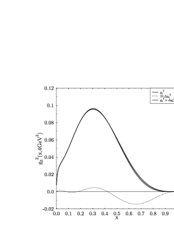
Figure 1: The fit for $g_{3}^{Z}$ (full line) and the corresponding renormalon contribution multiplied by a factor $10$ (dotted line). The dashed lines show the size of the ambiguity for $g_{3}^{Z}$, i. e. $g_{3}^{Z}\pm\Delta g_{3}^{Z}$.

Figure 2: The same as fig. 4 for $g_{5}^{Z}$.

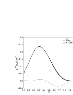
Figure 3: The same as fig. 4 for $g_{3}^{\gamma Z}$.

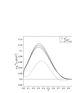
Figure 4: The same as fig. 4 for $g_{5}^{\gamma Z}$.

The deternination of all moments is equivalent to expressing $\Delta g_{j}(x)$ as a convolution

$$\Delta g_{j}(x)=\pm\left(\frac{\Lambda^{2}}{Q^{2}}\right)\frac{1}{\beta_{0}}\int_{x}^{1}\frac{\mathrm{d}y}{y}C_{j}^{IR1}(y)g(x/y)\;,$$ (29)

where the functions $C_{j}^{IR1}(y)$ defined by

$$\mbox{Res}\Big{(}B[C_{j,n}](s)\Big{)}\Bigg{|}_{s=1}=\int_{0}^{1}\mathrm{d}y\,y^{n}C_{j}^{IR1}(y)$$ (30)

are obtained from eqs. (20) and (21):

$$C_{3}^{IR1}(y)\!=\!\frac{C_{F}\mathrm{e}^{-c}}{(4\pi)^{2}}\left\{2\delta^{\prime}(y\!-\!1)\!-\!6\delta(y\!-\!1)\!+\!4\!+\!4y\!+\!16y^{2}\!-\!24y^{3}\!-\!\frac{4}{(1\!-\!y)_{+}}\right\},$$ (31)

$$C_{5}^{IR1}(y)\!=\!\frac{C_{F}\mathrm{e}^{-c}}{(4\pi)^{2}}\left\{2\delta^{\prime}(y\!-\!1)\!-\!10\delta(y\!-\!1)\!+\!8\!+\!4y\!+\!8y^{2}\!-\!\frac{8}{(1\!-\!y)_{+}}\right\},\hskip 34.14322pt$$ (32)

where $\frac{1}{(1-y)_{+}}$ is defined by $\int_{0}^{1}\mathrm{d}y\,f(y)\frac{1}{(1-y)_{+}}=\int_{0}^{1}\mathrm{d}y\frac{f(y)-f(1)}{1-y}$ . We use the quark distributions given in [24] and the parton model expressions

$$g_{3}^{Z} = 2x\sum_{q}g_{V}^{q}g_{A}^{q}(\Delta q-\Delta\overline{q})\;,$$ (33)

$$2xg_{5}^{Z} = g_{3}^{Z}\;,$$ (34)

$$g_{5}^{\gamma Z} = 2x\sum_{q}e^{q}g_{A}^{q}(\Delta q-\Delta\overline{q})\;,$$ (35)

$$2xg_{5}^{\gamma Z} = g_{5}^{\gamma Z}\>.$$ (36)

We choose the momentum transfer to be $Q^{2}=4\,\mathrm{GeV}^{2}$. The integrals in eq. (29) are evaluated numerically and the results are plotted in the figures 4 to 4.

We have thus completed our analysis of the renormalon ambiguities for all twist-2 structure functions.

Acknoledgement: This work was supported by BMBF.

References

[1]M. Dasgupta and B. R. Webber, Phys. Lett.B382 (1996) 273.
[2] E. Stein, M.Meyer-Hermann, L. Mankiewicz and A. Schäfer,
Phys. Lett.B376 (1996) 177.
[3] M. Meyer-Hermann, M. Maul, L. Mankiewicz, E. Stein and
A. Schäfer, Phys. Lett.B383 (1996) 463.
[4] M. Beneke and V. I. Zakharov, Phys. Rev. Lett.69 (1992) 2472.
[5] M. Beneke, Nucl. Phys.B405 (1993) 424.
[6] M. Beneke and V. M. Braun, Nucl. Phys.B426 (1994) 301.
[7] M. Beneke and V. M. Braun, Phys. Lett.B348 (1995) 513.
[8] V. M. Braun, QCD Renormalons and Higher Twist
Effects, hep-ph/9505317 (1995).
[9]
Yu. L. Dokshitzer and B. R. Webber, Phys. Lett.B352 (1995) 451;
Phys. Lett.B404 (1997) 321;
Yu. L. Dokshitzer, G. Marchesini and B. R. Webber, Nucl.
Phys.B469 (1996) 93;
M. Dasgupta and B. R. Webber, Nucl. Phys.B484 (1997) 247;
Eur. Phys. J.C1 (1998) 539;
M. Dasgupta, G. E. Smye and B. R. Webber, Power Corrections to
Fragmentation Functions in Non-Singlet Deep Inelastic Scattering,
hep-ph/9803382 (1998).
[10] A. H. Mueller, Phys. Lett.B308 (1993) 355.
[11] V. I. Zakharov, Nucl. Phys.B385 (1992) 452.
[12] G. ’t Hooft in The Whys of Subnuclear Physics,
International School of Subnuclear Physics, Erice, 1977 (Hrsg. A. Zichichi),
Plenum Press (1979) 943.
[13] F. J. Dyson, Phys. Rev.85 (1952) 631.
[14] I. I. Bigi, M. A. Shifman, N. G. Uralzev and
A. I. Vainsklein, Phys. Rev.D50 (1994) 2234.
[15] D. J. Broadhust and A. G. Grozin, Phys. Rev.D52 (1995) 4082.
[16] Patricia Ball, M. Beneke and V. M. Braun,
Nucl. Phys.B452 (1995) 563.
[17] M. Anselmino, P. Gambino and J. Kalinovski, Z. Phys.C64 (1994) 267.
[18] J. Blümlein and N. Kochelev, Phys. Lett.B381 (1996) 296.
[19] D. J. Gross and F. Wilczek, Phys. Rev.D9 (1974) 980.
[20] H. D. Politzer, Phys. Reports14 (1974) 129.
[21] G. ’t Hooft and M. Veltman, Nucl. Phys.B44
(1972) 189.
[22] W. A. Bardeen, A. J. Buras, D. W. Duke and T. Muta,
Phys. Rev.D18 (1978) 3998.
[23] T. Muta, Foundations of Quantum Chromodynamics,
World Scientific (1987).
[24] T. Gehrmann and W. J. Stirling, Phys. Rev.D53 (1996) 6100.