Jet Physics: Theoretical Overview

I review the status of fixed order jet Monte Carlos and briefly discuss the prospects for next-to-next-to-leading order calculations. I present a general purpose next-to-leading order Monte Carlo program for four jet event shape observables in electron-positron annihilation and present some estimates of the light jet mass and narrow jet broadening distributions. Finally, I discuss an estimate of the strong coupling constant using the measured energy evolution of the average value of event shape variables such as thrust and heavy jet mass.

1 Introduction and status of fixed order parton level calculations

In the last decade there has been enormous progress in using perturbative QCD to predict and describe events containing jets. At the simplest lowest-order (LO) level, each jet is the footprint of a hard, well separated parton produced in the event. Although the predicted rate is sensitive to the choices of renormalization and factorization scales, qualitative comparisons of data and theory are generally very good. Techniques for computing tree level multiparton scattering amplitudes are very advanced and reliable numerical Monte Carlo programs exist (see Table 1) for processes such as $p\bar{p}\to W+4$ jets $\!{}^{{\bf?}}$ which provides one of the main backgrounds for top quark detection at the TEVATRON. However, the bulk of events populate topologies with fewer jets and here a more quantitative description is required. To date, this has been largely achieved by improving the theoretical prediction to next-to-leading order (NLO).

The addition of NLO effects produces four important improvements over a LO estimate. First, the dependence on the unphysical renormalization and factrorization scales is reduced so that the normalization is more certain. Second, we begin to reconstruct the parton shower so that two partons may combine to form a single jet. As a result, jet cross sections become sensitive to the details of the jet finding algorithm, particularly the way in which the hadrons are combined to form the jet axis and energy, and to the size of a jet cone. This sensitivity is also seen in experimental results. Third, the calculation becomes more sensitive to detector limitations because radiation outside the detector is simulated. This can change leading order results considerably for quantities such as the missing transverse energy in events containing a $W$ boson. Fourth, the presence of infrared logarithms is clearly seen and regions where resummations are needed to improve the perturbative prediction can be identified.

Where possible, NLO estimates of QCD cross sections have become de rigeur and have allowed many tests of the underlying dynamics and measurements of, for example, the running strong coupling constant. For all types of experiment, NLO Monte Carlos are playing a vital role in making detailed comparisons with hadronic events. Some examples of NLO programs are listed in Table 1. Recent examples where disagreement between theory and experiment have yielded great excitement are the single jet inclusive data at CDF and the $W+1$ jet/ $W+0$ jet ratio measured by D0. For updates on these issues, I refer you to the talks by Elvira $\!{}^{{\bf?}}$ and Summers $\!{}^{{\bf?}}$.

However, one loop matrix elements rapidly become more difficult to compute as the number of external particles increases. In the last few years, a number of problems connected with one-loop integrals with five external particles have been solved and the one-loop scattering amplitudes for five parton $\!{}^{{\bf?}}$ and four partons and a vector boson $\!{}^{{\bf?},{\bf?}}$ have been computed. These matrix elements are relevant for $p\bar{p}\to 3$ jets, $e^{+}e^{-}\to 4$ jets, $ep\to 3+1$ jets and $p\bar{p}\to V+2$ jets. This latter process is likely to be very relevant at the TEVATRON in Run II, where associated Higgs production $p\bar{p}\to V+H$ followed by $H\to b\bar{b}$ is an eagerly anticipated discovery channel for the Higgs boson. NLO Monte Carlo programs for some of these processes are starting to appear $\!{}^{{\bf?},{\bf?}}$ and $\!{}^{{\bf?},{\bf?}}$ (see Table 1) and comparisons with experimental data are underway.

However, while the NLO program has been extremely successful in reducing the theoretical uncertainty, the improvements in the data are even more impressive, to the extent that the theoretical error tends to dominate. For example, in extracting the strong coupling from event shapes at LEP, the renormalization scale uncertainty engenders approximately a 5% uncertainty in $\alpha_{s}(M_{Z})$ while the experimental error is typically 2%. One way to improve the theoretical predictions is to incorporate next-to-next-to-leading order (NNLO) effects. This would reduce the renormalization scale uncertainty and also allow a better interface between the theoretical and experimental jet finding algorithms - now three partons will be able to merge to form the jet. Although a complete NNLO jet calculation is some way off, and for $2\to 2$ processes the two-loop double box integrals are not even known yet, some encouraging steps have been taken in this direction. For example, the singularity structures when two partons are unresolved has been examined $\!{}^{{\bf?}}$. More impressive is the recent calculation of the two-loop four gluon scattering amplitudes in a $N=4$ supersymmetric version of QCD $\!{}^{{\bf?}}$. While this result may not be directly relevant, the techniques developed to obtain it undoubtedly will be and I expect rapid progress in the evaluation of two loop QCD matrix elements. Much work will still be needed to turn the amplitudes into cross sections, but I predict that numerical NNLO programs will be available for $p\bar{p}\to\leq 2$ jets and $e^{+}e^{-}\to 3$ jets will be available within the next five years.

In the remainder of this talk, I will focus on two recent examples of theoretical progress in jet physics. First, I will discuss some new results for four jet event shape observables using the recent one loop matrix element calculations for $V\to 4~{}$partons $\!{}^{{\bf?},{\bf?}}$. Second, I will discuss how the theoretical error on the strong coupling may be reduced by considering average values of event shapes at a range of different centre-of-mass energies.

Order	External legs	Physical process	Program
LO	$\leq 7$ partons	$p\bar{p}\to\leq 5$ jets	NJETS $\!{}^{{\bf?}}$
LO	$V+\leq 6$ partons	$p\bar{p}\to W+\leq 4$ jets	VECBOS $\!{}^{{\bf?}}$
LO	$V+\leq 6$ partons	$p\bar{p}\to Z+4$ jets	$\!{}^{{\bf?}}$
LO	$V+\leq 6$ partons	$e^{+}e^{-}\to 6$ jets	$\!{}^{{\bf?}}$
NLO	4 partons	$p\bar{p}\to\leq 2$ jets	EKS $\!{}^{{\bf?}}$, JETRAD $\!{}^{{\bf?}}$
NLO	$V$ + 3 partons	$e^{+}e^{-}\to 3$ jets	EVENT $\!{}^{{\bf?}}$, EVENT2 $\!{}^{{\bf?}}$
NLO	$V$ + 3 partons	$p\bar{p}\to V+\leq 1$ jet	DYRAD $\!{}^{{\bf?}}$
NLO	$V$ + 3 partons	$ep\to 2+1$ jet	DISENT $\!{}^{{\bf?}}$, MEPJET $\!{}^{{\bf?}}$, DISASTER $\!{}^{{\bf?}}$
NLO	5 partons	$p\bar{p}\to 3$ jets	$\!{}^{{\bf?}}$, $\!{}^{{\bf?}}$
NLO	$V$ + 4 partons	$e^{+}e^{-}\to 4$ jets	MENLO PARC $\!{}^{{\bf?}}$, DEBRECEN $\!{}^{{\bf?}}$

Table 1: Available multi parton scattering matrix elements and some commonly used fixed order Monte Carlo implementations.

2 4 jet observables

As mentioned earlier, the one-loop matrix elements appropriate for the decay of a vector boson into four partons have recently been computed by two groups $\!{}^{{\bf?},{\bf?}}$. These matrix elements have been combined with the tree level amplitudes for the decay of a vector boson into five partons to compute the NLO corrections to a variety of four jet rates and event shapes by two groups; the programs MENLO PARC by Dixon and Signer $\!{}^{{\bf?}}$ and DEBRECEN by Trocsanyi and Nagy $\!{}^{{\bf?}}$. Here we report on results obtained using a third numerical implementation of these matrix elements to compute infrared safe four jet observables, EERAD2 $\!{}^{{\bf?}}$. This program uses the ‘squared’ one-loop matrix elements of $\!{}^{{\bf?}}$ together with squared tree level matrix elements for $\gamma^{*}\to 5$ partons. Both four and five parton contributions are singular in the infrared limit and there are several ways of performing the cancellation $\!{}^{{\bf?},{\bf?},{\bf?},{\bf?}}$. We use a modified version of the generic slicing approach $\!{}^{{\bf?}}$ that does not depend on the slicing parameter $y_{\min}$.

As a check of the numerical results, Table 2 shows the predictions for each of the three Monte Carlo programs for the four jet rate for three jet clustering algorithms; the Jade-E0, Durham $\!{}^{{\bf?}}$, and Geneva $\!{}^{{\bf?}}$ algorithms. We show results with $\alpha_{s}(M_{Z})=0.118$ for three values of the jet resolution parameter $y_{cut}$. There is good agreement with the results from the other two calculations.

Algorithm	$y_{{\rm cut}}$	MENLO PARC	DEBRECEN	EERAD2
	0.005	$(1.04\pm 0.02)\cdot 10^{-1}$	$(1.05\pm 0.01)\cdot 10^{-1}$	$(1.05\pm 0.01)\cdot 10^{-1}$
Durham	0.01	$(4.70\pm 0.06)\cdot 10^{-2}$	$(4.66\pm 0.02)\cdot 10^{-2}$	$(4.65\pm 0.02)\cdot 10^{-2}$
	0.03	$(6.82\pm 0.08)\cdot 10^{-3}$	$(6.87\pm 0.04)\cdot 10^{-3}$	$(6.86\pm 0.03)\cdot 10^{-3}$
	0.02	$(2.56\pm 0.06)\cdot 10^{-1}$	$(2.63\pm 0.06)\cdot 10^{-1}$	$(2.61\pm 0.05)\cdot 10^{-1}$
Geneva	0.03	$(1.71\pm 0.03)\cdot 10^{-1}$	$(1.75\pm 0.03)\cdot 10^{-1}$	$(1.72\pm 0.03)\cdot 10^{-1}$
	0.05	$(8.58\pm 0.15)\cdot 10^{-2}$	$(8.37\pm 0.12)\cdot 10^{-2}$	$(8.50\pm 0.06)\cdot 10^{-2}$
	0.005	$(3.79\pm 0.08)\cdot 10^{-1}$	$(3.88\pm 0.07)\cdot 10^{-1}$	$(3.87\pm 0.03)\cdot 10^{-1}$
JADE-E0	0.01	$(1.88\pm 0.03)\cdot 10^{-1}$	$(1.92\pm 0.01)\cdot 10^{-1}$	$(1.93\pm 0.01)\cdot 10^{-1}$
	0.03	$(3.46\pm 0.05)\cdot 10^{-2}$	$(3.37\pm 0.01)\cdot 10^{-2}$	$(3.35\pm 0.01)\cdot 10^{-2}$

Table 2: The four-jet fraction as calculated by MENLO PARC, DEBRECEN and EERAD2, for the different jet recombination schemes and varying $y_{\rm cut}$. The rate is normalized by the ${\cal O}(\alpha_{s})$ total hadronic cross-section, $\sigma_{\rm tot}=\sigma_{0}\,(1+\alpha_{s}/\pi)$.

In addition to the jet rates, there are also NLO predictions in the literature for four-jet event shapes such as the $D$ parameter, Acoplanarity and the Fox-Wolfram moments $\!{}^{{\bf?}}$. These variables vanish as the three jet limit approaches; i.e. as the event becomes more planar. Of course there are many other event shape variables that vanish as the event becomes more three jet like. Here, I focus on observables derived by dividing the event into two hemispheres $H_{1}$ and $H_{2}$ according to the orientation of the thrust axis $\vec{n}$ defined by,

$$T=\max\frac{\sum_{k}|\vec{p}_{k}.\vec{n}|}{\sum_{k}|\vec{p}_{k}|}.$$ (1)

Particles that satisfy $\vec{p}_{i}.\vec{n}>0$ are assigned to hemisphere $H_{1}$, while all other particles are in $H_{2}$. The light hemisphere mass, $m_{L}^{2}/s$, and the narrow jet broadening, $B_{\min}$, are defined by,

$$\frac{m_{L}^{2}}{s} = \frac{1}{s}\min_{i=1,2}\left(\sum_{k\in H_{i}}p_{k}\right)^{2}$$

$$B_{\min} = \min_{i=1,2}\frac{\sum_{k\in H_{i}}|\vec{p}_{k}\times\vec{n}|}{2\sum_{k}|\vec{p}_{k}|},$$ (2)

are both non-zero when there are at least four particles in the final state. These variables are related to the heavy jet mass $m_{H}^{2}/s$ and the wide jet broadening $B_{\max}$ which are obtained by maximising the quantities in Eq. 2, and which require at least three particles in the event to be non-zero.

The LO and NLO predictions for $m_{L}^{2}/s$ and $B_{\min}$ with a renormalization scale $\mu=M_{Z}$ and $\alpha_{s}(M_{Z})=0.1194$ are shown in fig. 1, together with data from $\!{}^{{\bf?}}$. At small values of the observable, we see the presence of large logarithms which must be resummed to obtain a meaningful result. At larger values, we see that the next-to-leading order corrections are large and approximately 100%. Similar large effects have been noted for other four jet observables $\!{}^{{\bf?},{\bf?}}$. While such large effects may make the perturbation theory appear unreliable, we note that effects of similar size have been noted for three jet event shapes like thrust $\!{}^{{\bf?},{\bf?}}$. This may be a sign that large higher order or power corrections are present. Or it may simply indicate that the physical scale $\mu=M_{Z}$ is a very poor choice of the renormalization scale, which itself engenders large ultraviolet logarithms in the higher order terms. In fact, such ultraviolet logarithms may be resummed using the FAC or fastest apparent convergence scale $\!{}^{{\bf?}}$. This scale is usually much less than the physical scale (and particularly so when the next-to-leading order corrections appear large) and may be disfavoured for that reason. However, the prediction using this scale (shown as dotted lines in fig. 1.) does lie much closer to the data.

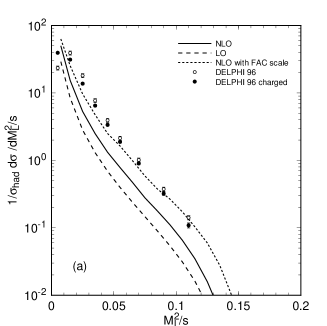
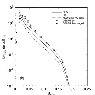
Figure 1: The (a) light hemisphere mass distribution $1/\sigma_{had}d\sigma/d(M_{L}^{2}/s)$ and (b) narrow jet broadening distribution $1/\sigma_{had}d\sigma/dB_{\min}$ at LEP energies. The LO (NLO) prediction is shown dashed (solid) for $\mu=M_{Z}$. The LO (and NLO) prediction using the FAC scale is shown as a dotted line. The data is taken from $\!{}^{{\bf?}}$.

3 Strong coupling from the energy evolution of event shapes

A vital ingredient in perturbative predictions is an accurate knowledge of the strong coupling constant. This can be determined via analysis of event shape variables at LEP. Consider the observable $R(Q)$ with a perturbation series and leading power correction that describes the hadronization phase of the hard scattering of the form,

$$R(Q)=a+r_{1}a^{2}+r_{2}a^{3}+\ldots+\frac{\lambda}{Q}(1+\lambda_{1}a+\ldots),$$ (3)

where $a\equiv\alpha_{S}(\mu)/\pi$ denotes the renormalization group improved coupling. Note that the normalization is simply such that the perturbative expansion begins with unit coefficient. An example of such a variable is $R(Q)=<\!\!1-T\!\!>/1.05$, where in the ${\overline{MS}}$ scheme with $\mu=Q$ and $N_{f}=5$ active quark flavours the NLO coefficient is $r_{1}=9.70$ $\!{}^{{\bf?},{\bf?}}$. The NNLO coefficient $r_{2}$ is as yet unknown. The precise form of the power corrections is as yet not fully understood, but, for the purposes of comparison with data, may be parameterized in a variety of different ways $\!{}^{{\bf?}}$. To extract $\alpha_{s}(M_{Z})$ from the data, we just truncate the perturbative series for a given renormalization scale $\mu=xQ$ (which is typically $x=1$). In other words, we assume the higher order term $r_{2}\equiv 0$, $r_{3}\equiv 0$ etc. Then, by comparing with experimental data, we solve for $a$. A recent analysis $\!{}^{{\bf?}}$ for $<\!\!1-T\!\!>$ using the power correction model of $\!{}^{{\bf?}}$ finds,

$$\alpha_{s}(M_{Z})=0.1204\pm 0.0013\phantom{~{}}^{+0.0061}_{-0.0050}\phantom{~{}}{}^{+0.0023}_{-0.0018},$$ (4)

(with a $\chi^{2}/{\rm d.o.f}$ of $42.6/24$) where the first error is purely experimental. The second and third errors come from varying the theoretical input parameters, first varying the renormalization scale $x$ between 0.5 and 2 and second the parameters of the power correction model. Clearly the estimate of the theoretical error is dominated by the renormalization scale uncertainty. Similar results are presented in $\!{}^{{\bf?}}$.

Alternatively, we may avoid the renormalization scale entirely and directly write an expression for the running of $R(Q)$ with $Q$ in terms of $R(Q)$ itself $\!{}^{{\bf?},{\bf?}}$,

$$\frac{dR}{d\log Q} = -bR^{2}(1+cR+\rho_{2}R^{2}+\ldots)+K_{0}R^{-c/b}e^{-1/bR}(1+K_{1}R+\ldots)+\ldots$$ (5)

$$\equiv -b\rho(R).$$

Here $b$ and $c$ are the first two universal terms of the QCD beta-function,

$$b=\frac{33-2N_{f}}{6},\qquad\qquad c=\frac{153-19N_{f}}{12b}.$$ (6)

The quantity,

$$\rho_{2}\equiv r_{2}+c_{2}-r_{1}c-r_{1}^{2},$$ (7)

is a renormalization scheme and renormalization scale (RS) invariant combination of the NLO and NNLO perturbation series and beta-function coefficients with, in the $\overline{MS}$ scheme,

$$c_{2}=\frac{77139-15099N_{f}+325N_{f}^{2}}{1728b}.$$ (8)

Since the NNLO $r_{2}$ is unknown, so is $\rho_{2}$. The coefficient $K_{0}$ is directly related to the coefficient $\lambda$ of the $1/Q$ power corrections in eq. (3).

Since $R(Q)$ and $dR/d\log Q$ are both observables one could in principle directly fit eq. (5) to the data and thus constrain the unknown coefficients $\rho_{2}$ and $K_{0}$. At asymptotic energies all observables run universally according to,

$$\frac{dR}{d\log Q}=-bR^{2}(1+cR),$$ (9)

and one could see how close the data are to this evolution equation. Given the error bars of the data and the separation in $Q$ of the different experiments it is preferable, however, to integrate up eq. (5) using asymptotic freedom ($R(Q)\to 0$ as $Q\to\infty$) as a boundary condition. In this way one obtains,

$$\frac{1}{R}+c\log\left(\frac{cR}{1+cR}\right)=b\log\left(\frac{Q}{\Lambda_{R}}\right)-\int_{0}^{R}dx\,\left(-\frac{1}{\rho(x)}+\frac{1}{x^{2}(1+cx)}\right),$$ (10)

where $\Lambda_{R}$ is a constant of integration. By comparing with the $Q\to\infty$ behaviour of eq. (3) one can deduce that $\Lambda_{R}$ is related to $\Lambda_{\overline{MS}}$,

$$\Lambda_{R}=e^{r/b}\left(\frac{2c}{b}\right)^{-c/b}\Lambda_{\overline{MS}},$$ (11)

where $r\equiv r_{1}^{\overline{MS}}(\mu=Q)$.

If we assume that the right-hand side of eq. (5) is adequately parameterized by,

$$-b\rho(R)=-bR^{2}(1+cR+\rho_{2}R^{2})+K_{0}R^{-c/b}e^{-1/bR},$$ (12)

we can then insert this form into eq. (10) and by (numerically) solving the transcendental equation, perform fits of $\rho_{2}$, $K_{0}$ (or equivalently $\lambda$) and $\Lambda_{\overline{MS}}$ to the data $R(Q)$.

Fig. 2(a) shows the fit to the data (dashed line) obtained by setting $\rho_{2}=\lambda=0$. This corresponds to the universal running of the observable given in eq. (9). The fitted value is $\Lambda_{\overline{MS}}^{(5)}=266~{}{\rm MeV}$ with a $\chi^{2}/{\rm d.o.f}=81.7/32$. We clearly see that the data is falling much too quickly with increasing $Q$ for the asymptotic behaviour to have set in at these scales. The data favours a more steeply falling evolution which could be caused by either higher order corrections with a positive $\rho_{2}$, or power corrections with non-zero $K_{0}$. We therefore perform a 3-parameter fit allowing $\rho_{2}$, $K_{0}$ and $\Lambda_{\overline{MS}}$ to vary independently which is shown as a solid line in Fig. 2(a). The minimum $\chi^{2}$ fit is acceptable ($\chi^{2}/{\rm d.o.f}=40.4/30$) and estimating an error by allowing $\chi^{2}$ within $1$ of the minimum gives,

$$\Lambda_{\overline{MS}}^{(5)}=245^{+20}_{-17}~{}{\rm MeV}\qquad{\rm with}\qquad\rho_{2}=-16\mp 11\qquad{\rm and}\qquad\lambda=0.27^{+0.12}_{-0.10}~{}{\rm GeV}.$$

These values of $\rho_{2}$ and $\lambda$ are reasonably small, thereby lending support to our critical assumption that the evolution equation could be parameterized in this way. Converting the extracted value of $\Lambda_{\overline{MS}}$ into $\alpha_{S}(M_{Z})$ we find,

$$\alpha_{S}(M_{Z})=0.1194\pm 0.0014.$$ (13)

We see that our central value is remarkably close to that obtained by $\!{}^{{\bf?},{\bf?}}$. The main difference is in how the errors are determined. In our approach, the errors are estimated by allowing the uncalculated higher orders to be fitted by the data and the data prefers these to be small. In particular, the renormalization group scale-dependent logarithms are automatically resummed to all orders on integrating eq. (5) and do not add a spurious extra large uncertainty in the extraction of $\Lambda_{\overline{MS}}$ (or equivalently $\alpha_{s}(M_{Z})$). As higher order corrections become known, the new RS-invariant terms, $\rho_{2}$, $\rho_{3}$ etc., can be incorporated and the fit refined.

With such an accurate value of $\alpha_{S}(M_{Z})$, we should expect that applying this approach to other variables should yield consistent results. Unfortunately, the method described here relies on having reliable data over a wide range of $Q$ values. This limits its use to a very few variables, like thrust or the heavy jet mass. If we repeat the same analysis for the average of the heavy jet mass, $<\!\!m_{H}^{2}/s\!\!>$, we find that a one parameter fit with $\rho_{2}=\lambda=0$ gives a very poor fit, $\chi^{2}/{\rm d.o.f}=213/29$ and $\Lambda_{\overline{MS}}=368$ MeV. As seen in Fig. 2(b) the data evolves much faster than the QCD prediction. However, allowing both $\rho_{2}$ and $\lambda$ to vary while using the value of $\Lambda_{\overline{MS}}=245$ MeV obtained from the $<\!\!1-T\!\!>$ analysis gives a much more satisfactory description. Here, $\chi^{2}/{\rm d.o.f}=40.3/27$ while $\rho_{2}=13$ and $\lambda=0.11$ GeV are sufficiently small to support our choice of parameterization.

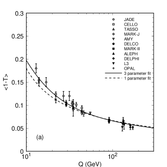
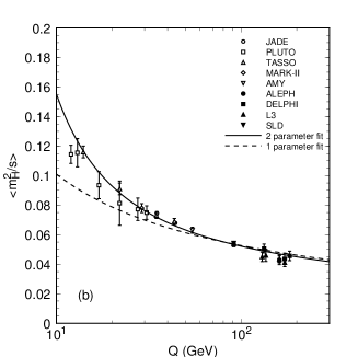
Figure 2: The average value of (a) 1-Thrust and (b) heavy jet mass obtained experimentally compared with the expectation of eq. (10). The dashed lines show the fit to the data with $\rho_{2}=\lambda=0$ while in (a) the result of the three parameter fit (to $\Lambda_{\overline{MS}},~{}\rho_{2}$ and $\lambda$) is shown as a solid line. In (b), the solid line shows the result of a two parameter fit (to $\rho_{2}$ and $\lambda$) using the value of $\Lambda_{\overline{MS}}$ obtained from the three parameter fit to $<\!\!1-T\!\!>$.

4 Outlook

The last decade has seen enormous progress both experimentally and theoretically in understanding high energy hadronic events. In many cases, we now have a quantitative understanding of the rates for strong interaction processes and detailed predictions for the structure of the events. One of the main theoretical uncertainties remains the renormalization scale uncertainty and the value of the strong coupling. New techniques for next-to-next-to-leading predictions are in sight and will help to reduce this error. However, a more immediate improvement may be obtained by resumming the ultraviolet logarithms explicitly.

References

References

- [1] F.A. Berends, H. Kuijf, J.B. Tausk and W.T. Giele, Nucl. Phys. B357 (1991) 32.
- [2] V.D. Elvira, these proceedings.
- [3] D.J. Summers, these proceedings.
- [4] Z. Bern, L. Dixon and D.A. Kosower, Phys. Rev. Lett. 70 (1993) 2677; Z. Kunszt, A. Signer and Z. Trócsányi, Phys. Lett. B336 (1994) 529; Z. Bern, L. Dixon and D.A. Kosower, Nucl. Phys. B437 (1995) 259
- [5] E.W.N. Glover and D.J. Miller, Phys. Lett. B396 (1997) 257; J.M. Campbell, E.W.N. Glover and D.J. Miller, Phys. Lett. B409 (1997) 503.
- [6] Z. Bern, L. Dixon and D.A. Kosower, Nucl. Phys. Proc. Suppl. 51C (1996) 243; Z. Bern, L. Dixon, D.A. Kosower and S. Weinzierl, Nucl. Phys. B489 (1997) 3; Z. Bern, L. Dixon and D.A. Kosower, Nucl. Phys. B513 (1998) 3
- [7] W.B. Kilgore and W.T. Giele, Phys. Rev. D55 (1997) 7183; W.B. Kilgore, in Proceedings of 32nd Rencontres de Moriond; QCD and High Energy Hadronic Interactions, Les Arcs, France, March 1997, hep-ph/9705384.
- [8] Z. Trócsányi, Phys. Rev. Lett. 77 (1996) 2182.
- [9] A. Signer and L. Dixon, Phys. Rev. Lett. 78 (1997) 811; A. Signer and L. Dixon, Phys. Rev. D56 (1997) 4031; A. Signer, Comput. Phys. Comm. 106 (1997) 125; A. Signer, hep-ph/9705218.
- [10] Z. Nagy and Z. Trócsányi, Phys. Rev. Lett. 79 (1997) 3604; hep-ph/9708343; hep-ph/9708344; hep-ph/9712385.
- [11] F.A. Berends and W.T. Giele, Nucl. Phys. B313 (1989) 595; S. Catani, Proceedings of Workshop on ‘New Techniques for Calculating Higher Order QCD Corrections’, preprint ETH-TH/93-01, Zurich (1992); J.M. Campbell and E.W.N. Glover, hep-ph/9710255; S. Catani, hep-ph/9802439.
- [12] Z. Bern, J.S. Rozowsky and B. Yan, Phys. Lett. B410 (1997) 273,
- [13] F.A. Berends, W.T. Giele and H. Kuijf, Phys. Lett. B232 (1989) 266: F.A. Berends and H. Kuijf, Nucl. Phys. B353 (1991) 59.
- [14] V. Barger, E. Mirkes, R.J.N. Phillips and T. Stelzer, Phys. Lett. B338 (1994) 336.
- [15] S. Moretti, Phys. Lett. B420 (1998) 367.
- [16] S.D. Ellis, Z. Kunszt and D.E. Soper, Phys. Rev. D40, 2188 (1989); Phys. Rev. Lett. 64, 2121 (1990); Phys. Rev. Lett. 69, 1496 (1992).
- [17] W.T. Giele, E.W.N. Glover and D.A. Kosower, Nucl. Phys. B403 (1993) 633.
- [18] Z. Kunszt, P. Nason, G. Marchesini and B.R. Webber, in Z Physics ar LEP 1, vol. 1, ed. G. Altarelli, R. Kleiss and C. Verzegnassi, CERN Yellow Report 89-08.
- [19] S. Catani and M.H. Seymour, Phys. Lett. B378 (1996) 287; Nucl. Phys. B485 (1997) 291.
- [20] E. Mirkes and D. Zeppenfeld, Phys. Lett. B380 (1996) 205.
- [21] D. Graudenz, hep-ph/9708362.
- [22] J.M. Campbell, M. Cullen and E.W.N. Glover, in preparation
- [23] K. Fabricius, I. Schmitt, G. Kramer and G. Schierholz, Z. Phys. C11 (1981) 315; W.T. Giele and E.W.N. Glover, Phys. Rev. D46 (1992) 1980.
- [24] R.K. Ellis, D.A. Ross and A.E. Terrano, Nucl. Phys. B178 (1981) 421.
- [25] S. Frixione, Z. Kunszt and A. Signer, Nucl Phys. B467 (1996) 399; Z. Nagy and Z. Trócsányi, Nucl. Phys. B486 (1997) 189.
- [26] Yu.L. Dokshitzer, Contribution to the Workshop on Jets at LEP and HERA, J. Phys. G17 (1991) 1441.
- [27] S. Bethke, Z. Kunszt, D.E. Soper and W.J. Stirling, Nucl. Phys. B370 (1992) 310.
- [28] P. Abreu et al, DELPHI Collaboration, Z. Phys. C73 (1996) 11.
- [29] D. Wicke, these proceedings.
- [30] A. Dhar and V. Gupta, Phys. Rev. D29 (1984) 2822; D.T. Barclay, C.J. Maxwell and M.T. Reader, Phys. Rev. D49 (1994) 3480; C.J. Maxwell, Phys. Lett. B409 (1997) 450.
- [31] P.A. Movilla Fernández et al and the JADE Collaboration, Eur. Phys. J. C1 (1998) 461.
- [32] J.M. Campbell, E.W.N. Glover and C.J. Maxwell, hep-ph/9803254.
- [33] Yu.L. Dokshitzer and B.R. Webber, Phys. Lett. B352 (1995) 451.
- [34] G. Grunberg, Phys. Lett. B95 (1980) 70; Phys. Rev. D29 (1984) 2315.