TTP 98–20

Improved Unitarity Bounds for $\bar{B}^{0}\to\pi^{+}\ell^{-}\bar{\nu}_{\ell}$ Decays

Thomas Mannel and Boris Postler

Institut für Theoretische Teilchenphysik,Universität Karlsruhe,
D – 76128 Karlsruhe, Germany.

We obtain model independent bounds for the form factors which arise in semileptonic $B\to\pi$ decays. To this end we derive a theoretical restriction for possible combinations of the value of the form factor and its derivatives at the end point region. These restrictions are then used as an input in a — slightly modified — general formalism, which has already been deduced and applied in earlier publications. Our results can be used to set constraints on the form factors which have to be obeyed by all model dependent parametrizations.

1 Introduction

One important parameter for the determination of the unitarity triangle of the CKM matrix is $V_{ub}$. While its phase can only be determined from non–leptonic decays, its magnitude will be determined from semileptonic processes. Various methods have been proposed to extract $V_{ub}$ from both inclusive as well as exclusive semileptonic decays, and the final numbers after the era of the $B$ factories will probably be obtained from a mixture of both exclusive and inclusive methods.

The disadvantage of exclusive decays is their dependence on form factors which are nonperturbative quantities. Modelling these form factors necessarily introduces some uncontrollable systematic uncertainty into the determination of $V_{ub}$ and hence a model independent method is desirable. At present the values of $V_{ub}$ extracted from exclusive semileptonic $B\to\pi$ decays using lattice QCD, QCD sum rules and quark models range from $|V_{ub}|=(2.5-4.5)\times 10^{-3}$. Clearly this is not a satisfactory situation, in particular in view of the data to be expected from the $B$ factories. Although there have been recent efforts to update existing models (see e.g. [1]–[4]), there is still room for some improvement.

There are constraints on form factors originating from their analyticity properties and the unitarity of the underlying theory. The ideas how to implement these constraints are in fact quite old [5]–[9] and have recently attracted renewed attention. In particular, combining these unitarity bounds with lattice data [10] has lead to relatively tight and model independent bounds on the form factors of $B\to\pi$ transitions.

In the present paper we improve the application of unitarity bounds in such a way that not only points at which the form factor is known (e.g. from lattice data or heavy quark relations) can be included, but also the slope and higher derivatives at some point, which could be known for instance from sum rule considerations. At the point of maximal momentum transfer the derivatives are correlated with the value of the form factor due to analyticity and we shall discuss the restrictions obtained from this in some detail.

A similar improvement of the unitarity bounds has been proposed by Boyd et al. [11, 12], where the form factors for $B\to\pi\ell\nu$ are expanded in a cleverly chosen conformal variable $z$ and some of the relations we use in the present paper appear in a similar form in these references.

In the next section we shall summarize the formalism as described in [9]. The improved bounds are considered in section 3 where we generalize the method to include known slopes and higher derivatives. We make use of the correlation between the derivatives and the value of the form factor taken at $q^{2}_{max}$ to tighten the bounds even without using any additional physics input. In order to get useful bounds some physics input is necessary and we chose to use the chiral limit which is valid close to the end point. This has a strong effect since any knowledge of the form factors in the end point region tightens the bounds significantly. With this input we study numerical examples.

2 Bounds on Form Factors

For later use we summarize in this section the formalism how to derive bounds on the form factors using only perturbative QCD, unitarity and the analyticity of the form factors in the complex plane.

We choose to describe the hadronic matrix element of the semileptonic $\bar{B}^{0}\to\pi^{+}\ell^{-}\bar{\nu}_{\ell}$ decays with the following two form factors:

$$\langle\pi^{+}(p^{\prime})|V^{\mu}|\bar{B}^{0}(p)\rangle = \left(p^{\mu}+{p^{\prime}}^{\mu}-\frac{M^{2}-m^{2}}{q^{2}}q^{\mu}\right)f^{+}(q^{2})$$

$$+\frac{M^{2}-m^{2}}{q^{2}}q^{\mu}f^{0}(q^{2})$$

where $M^{2}=m_{B}^{2}$, $m^{2}=m_{\pi}^{2}$, $V^{\mu}=\bar{u}\gamma^{\mu}b$ and $q=p-p^{\prime}$. In this notation $q^{2}$ runs from $q^{2}_{min}=m_{\ell}^{2}$ to $q^{2}_{max}=(M-m)^{2}$. Throughout this paper we will neglect the lepton masses and therefore set $q^{2}_{min}=0$. Furthermore, this special choice of decomposition into Lorentz vectors leads to form factors which have to satisfy the kinematical constraint

$$f^{+}(0)=f^{0}(0).$$ (2)

The form factors are real functions of a real variable but it is convenient to think of them as analytic functions in the complex $q^{2}$–plane.

To derive bounds on $f^{+}(q^{2})$ and $f^{0}(q^{2})$ we consider the two–point function

$$\Pi^{\mu\nu} \equiv i\int\mbox{d}^{4}{x}\enspace\mbox{e}^{iq\cdot x}\langle 0|T\{V^{\mu}(x)V^{\nu\dagger}(0)\}|0\rangle$$ (3)

$$\equiv -(g^{\mu\nu}q^{2}-q^{\mu}q^{\nu})\Pi_{T}(q^{2})+q^{\mu}q^{\nu}\Pi_{L}(q^{2}),$$

where $V^{\mu}=\bar{u}\gamma^{\mu}b$ as above and with $\Pi_{T/L}(q^{2})$ corresponding to the propagation of a $J^{P}=1^{-}/0^{+}$ particle. This two–point function can be (and has been) reliable evaluated in the deep euclidean region where $-q^{2}\equiv Q^{2}\gg\Lambda^{2}_{\mbox{\scriptsize QCD}}$, i.e. at an energy scale where perturbative QCD is appliccable.

Including a sum over all possible intermediate states $\Gamma$ we get the following result for the imaginary part of (3):

$$-(g^{\mu\nu}q^{2}-q^{\mu}q^{\nu})\mbox{ Im}{\Pi_{T}(q^{2})}+q^{\mu}q^{\nu}\mbox{ Im}{\Pi_{L}(q^{2})}$$

$$=\frac{1}{2}\sum_{\Gamma}(2\pi)^{4}\delta^{(4)}(q-p_{\gamma})\langle 0|V^{\mu}(0)|\Gamma\rangle\langle\Gamma|V^{\nu\dagger}(0)|0\rangle.$$ (4)

We therefore get an equation for the spectral functions $\mbox{ Im}{\Pi_{T/L}(q^{2})}$ (i.e. for the absorptive parts of $\Pi_{T/L}(q^{2})$) which we can relate to the real parts using the substracted dispersion relations

$$\chi_{L}(Q^{2})\equiv\left(-\frac{\partial}{\partial Q^{2}}\right)(-Q^{2}\Pi_{L}(Q^{2}))=\frac{1}{\pi}\int_{0}^{\infty}\mbox{d}{t}\enspace\frac{t\mbox{ Im}{\Pi_{L}(t)}}{(t+Q^{2})^{2}}$$ (5)

and

$$\chi_{T}(Q^{2})\equiv\frac{1}{2}\left(-\frac{\partial}{\partial Q^{2}}\right)^{2}(-Q^{2}\Pi_{T}(Q^{2}))=\frac{1}{\pi}\int_{0}^{\infty}\mbox{d}{t}\enspace\frac{t\mbox{ Im}{\Pi_{T}(t)}}{(t+Q^{2})^{3}}.$$ (6)

We now restrict ourselves to include only contributions of the $B^{*}$ and the $B\pi$ states in the sum over all intermediate states in (2). It is possible to discard all other intermediate states because (2) is a sum of positive terms if the indices are treated symmetrically. Using isospin and crossing symmetry we can use (2) to express (2) by the two form factors. Projecting out now the transversal/longitudinal parts, one gets the inequalities

$$\mbox{ Im}{\Pi_{L}(t)}\geq\frac{3}{2}\frac{t_{+}t_{-}}{16\pi}\sqrt{(t-t_{+})(t-t_{-})}\frac{|f^{0}(t)|^{2}}{t^{3}}\Theta(t-t_{+})$$ (7)

and

$$\mbox{ Im}{\Pi_{T}(t)} \geq \pi\left(\frac{m_{B^{*}}}{f_{B^{*}}}\right)^{2}\delta(t-m_{B^{*}}^{2})$$ (8)

$$+ \frac{3}{2}\frac{1}{48\pi}\frac{[(t-t_{+})(t-t_{-})]^{3/2}}{t^{3}}|f^{+}(t)|^{2}\Theta(t-t_{+}),$$

where $t=q^{2}$ and $t_{\pm}=(M\pm m)^{2}$.

It is now possible to get bounds on the form factors if one inserts (7,8) in (5,6). Since the l.h.s. of (5,6) can be calculated for $Q^{2}\gg\Lambda^{2}_{\mbox{\scriptsize QCD}}$ using perturbative QCD one gets inequalities which restrict the form factors. These inequalities take the form (in shorthand notation)

$$J(Q^{2})\geq\frac{1}{\pi}\int_{t_{+}}^{\infty}\mbox{d}{t}\enspace k(t,Q^{2})|f(t)|^{2}$$ (9)

where $J(Q^{2})$ denotes the QCD input (i.e. the perturbative calculation of $\chi_{T/L}$) including the $B^{*}$–resonance in case of $f^{+}$ and $k(t,Q^{2})$ is a known kinematical function. The exact value/structure of $J(Q^{2})$ and $k(t,Q^{2})$ does of course depend on the form factor under examination.

To translate the inequality (9) in constraints on the form factor for values of $t$ in the range $[0,t_{-}]$ (which is the kinematical region of physical interest), we map the complex $t$–plane into the unit disc with the conformal transformation

$$\frac{1+z}{1-z}=\sqrt{\frac{t_{+}-t}{t_{+}-t_{-}}}$$ (10)

so that (9) becomes

$$J(Q^{2})\geq\int_{|z|=1}\frac{\mbox{d}z}{2\pi iz}|\phi(z,Q^{2})f(z)|^{2}$$ (11)

with $f(z)\hat{=}f(t(z))$. Here we have used the fact, that $k(t,Q^{2})$ is a positive definite quantity so that $\phi(z,Q^{2})\equiv\sqrt{k(t(z),Q^{2})}$ times the squareroot of the Jacobian of the transformation.

The value of the form factor $f(z)$ for any point $z(t)$ is accessible by defining an inner product

$$\langle g|h\rangle=\int_{|z|=1}\frac{\mbox{d}z}{2\pi iz}\bar{g}(z)h(z)$$ (12)

and by considering the product $\langle g_{t}|\phi f\rangle$ where

$$g_{t}=\frac{1}{1-\bar{z}(t)z},$$ (13)

so that $f(z(t))$ has no poles in the range $[0,t_{-}]$. Cauchy’s theorem now yields

$$\langle g_{t}|\phi f\rangle=\phi(z(t),Q^{2})f(z(t)).$$ (14)

On the other hand, if there is a pole at $t=t_{p}$ away from the cut in the complex $t$–plane (i.e. for $t>t_{-}$), one would obtain

$$\langle g_{t}|\phi f\rangle=\phi(z(t),Q^{2})f(z(t))+\frac{\mbox{Res}\{\phi f,z(t_{p})\}}{z(t_{p})-z(t)}.$$ (15)

The residue can either be approximated or eliminated completely by the transformation [13]

$$\phi(z,Q^{2})\quad\to\quad\phi_{p}(z,Q^{2})\equiv\phi(z,Q^{2})\frac{z-z(t_{p})}{1-\bar{z}(t_{p})z}$$ (16)

where $t_{p}$ is assumed to lie in the range $[t_{-},t_{+}]$ so that $\phi_{p}$ is positive for $z=z(t)$ with $t$ in $[0,t_{-}]$. This replacement cancels the pole of $f(t)$ so that (14) holds. The crucial property of this transformation is the fact that, since $|(z-z(t_{p}))/(1-\bar{z}(t_{p})z)|=1$ for $z$ on the unit circle, $\langle\phi f|\phi f\rangle=\langle\phi_{p}f|\phi_{p}f\rangle$ and the QCD constraints are left unchanged.

Figure 1: Bounds on the form factors $f^{0}(t)$ (on the left side, $t$ increasing to the left) and $f^{+}(t)$ (on the right side), derived without any additional constraints and plotted over the whole kinematical range of $[0,t_{-}]$ ($t$ in $\mbox{GeV}^{2}$).

Because of the positivity of the inner product we have

$$\mbox{det}\left({\begin{array}[]{cc}\langle\phi f|\phi f\rangle&\langle\phi f|g_{t}\rangle\\ \langle g_{t}|\phi f\rangle&\langle g_{t}|g_{t}\rangle\end{array}}\right)\geq 0,$$ (19)

which, by eliminating $\langle\phi f|\phi f\rangle$ with (11), gives us the following bounds on the form factors

$$|f(t)|^{2}\leq J(Q^{2})\frac{1}{1-z^{2}(t)}\frac{1}{|\phi(z(t),Q^{2})|^{2}}$$ (20)

where we have made use of the fact that $z(t)$ is real for $t$ in $[0,t_{-}]$.

These Bounds, which are derived using only perturbative QCD and which do not depend on any model assumptions or input parameters (they are therefore quite loose), are plotted in figure 1. They were calculated using $Q^{2}=0$ in $J(Q^{2})$ at order ${\cal O}(\alpha_{s})$

If we know the value of the form factor $f_{i}\equiv f(t_{i})$ at $n$ points $i=1,\dots,n$, we can define a matrix $\cal{M}$

$$\cal{M}=\left(\begin{array}[]{ccccc}\langle\phi f|\phi f\rangle&\langle\phi f|g_{t}\rangle&\langle\phi f|g_{t_{1}}\rangle&\cdots&\langle\phi f|g_{t_{n}}\rangle\\ \langle g_{t}|\phi f\rangle&\langle g_{t}|g_{t}\rangle&\langle g_{t}|g_{t_{1}}\rangle&\cdots&\langle g_{t}|g_{t_{n}}\rangle\\ \langle g_{t_{1}}|\phi f\rangle&\langle g_{t_{1}}|g_{t}\rangle&\langle g_{t_{1}}|g_{t_{1}}\rangle&\cdots&\langle g_{t_{1}}|g_{t_{n}}\rangle\\ \vdots&\vdots&\vdots&\ddots&\vdots\\ \langle g_{t_{n}}|\phi f\rangle&\langle g_{t_{n}}|g_{t}\rangle&\langle g_{t_{n}}|g_{t_{1}}\rangle&\cdots&\langle g_{t_{n}}|g_{t_{n}}\rangle\end{array}\right)$$ (26)

and obtain, using again the positivity of the inner product,

$$\det{\cal M}\geq 0.$$ (27)

Since $\langle\phi f|\phi f\rangle$ is eliminated using (11) and since all components except $f(t)$ of this matrix are known — they are either constants or functions of $t$ — the inequality (27) leads to bounds on the form factors $f(t)$. The inclusion of some known values (which i.e. are predicted by a model or which one can get by lattice calculations, see [10]) therefore will give us more stringent bounds

$$F_{lo}(t,t_{i},f_{i})\leq f(t)\leq F_{up}(t,t_{i},f_{i})$$ (28)

with $F_{lo}$ and $F_{up}$ calculable functions of $t$ with the parameters $t_{i},f_{i}$.

The upper and lower bounds can be written as

$$F_{up,lo}(t,Q^{2})=\frac{-\beta(t)\pm\sqrt{c(Q^{2})\cdot\Delta(t)}}{\alpha\cdot\phi(t,Q^{2})}.$$ (29)

The shape of $F_{up,lo}(t,Q^{2})$ as functions of $t$ depend on the values for $t_{i}$ and $f_{i}$. In (29), $\alpha$ is a scaling constant, $\beta(t)$ gives roughly the shape of the form factor while the squareroot in (29) distinguishes the upper from the lower bound. In the squareroot, $c(Q^{2})$ is a constant in $t$ which depends only on the energy scale $Q^{2}$, and $\Delta(t)$ is a function with zeros in every $t_{i}$. The reason why the function $\Delta(t)$ should behave like this is quite clear: since we fixed the value of the form factor at certain points $t_{i}$, the upper and lower bound should coincide in these points (for an exact definition of the functions appearing in (29) see [10]).

3 Improving the Bounds

The method of including ‘fixed points’ (i.e. to fix the value of the form factor at certain kinematical points) which we summarized in 2 is well known and used throughout the literature. However, this formalism can be applied in a slightly different way: to include the slope or even higher derivatives of the form factor. This is desirable because it is possible to obtain the slope e.g. for low $t$ from QCD sum rules or for $t$ near the kinematical end point from the chiral limit.

Consider two fixed points $t_{1}$ and $t_{2}=t_{1}+\epsilon$ with $\epsilon$ arbitrary but small. We get the coresponding values of $f(t_{i})$ via a Taylor expansion:

$$f(t_{1}) \equiv f_{1}$$ (30)

$$f(t_{2}) = f(t_{1})+\epsilon\left.\frac{d}{dt}f(t)\right|_{t=t_{1}}\,.$$ (31)

We can now calculate the bounds depending on these values for $t_{1},t_{2},f_{1}$ and $f_{2}$ and take the limit $\epsilon\to 0$. It is useful to define a function $\psi(z,Q^{2})\equiv f(z)\phi(z,Q^{2})$, in terms of which we obtain

$$\psi_{up,lo} = \frac{(1-z_{1}^{2})(\psi_{1}(1-2zz_{1}+z_{1}^{2})+\psi_{1}^{\prime}(z-z_{1})(1-z_{1}^{2}))}{(1-zz_{1})^{2}}$$

$$\pm \frac{(1-z_{1}^{2})(z-z_{1})^{2}}{(1-zz_{1})^{2}\sqrt{1-z^{2}}}\times$$

$$\sqrt{J-\psi_{1}^{2}(1+z_{1}^{2})+2\psi_{1}\psi_{1}^{\prime}z_{1}(1-z_{1}^{2})-[\psi_{1}^{\prime}]^{2}(1-z_{1}^{2})^{2}}$$

where $z_{1}\equiv z(t_{1})$, $\psi_{1}\equiv\psi(z_{1},Q^{2})$ and

$$\psi_{1}^{\prime}=\left.\frac{\partial}{\partial z}\psi(z,Q^{2})\right|_{z=z_{1}}\,.$$

It is obvious how to extend this to higher derivatives (including e.g. the curvature of the form factor), but the corresponding equations become tedious. In parts of the numerical analysis presented below the curvature has been included.

It has been observed (see [11, 12] and [14, 15]) that the inequality (11) also yields restrictions for the derivatives of the form factor in the end point $t_{-}$. We shall use this input to restrict the possible values of the form factor at $t_{-}$ in terms of the slope and the curvature. In order to do this we rewrite (11) into the form

$$\frac{1}{2\pi}\int_{0}^{2\pi}\mbox{d}{\Theta}\enspace|\psi(\mbox{e}^{i\Theta})|^{2}\leq J(Q^{2}).$$ (33)

In the case of $f^{0}$ it is now possible to perform a Taylor expansion around $z_{0}=0$ ($t=t_{-}$) which is convergent in the full unit disc, since $f^{0}$ does not have poles or cuts in this region. This is due to the fact that no physical intermediate states can contribute. We therefore get the inequality

$$J(Q^{2})\geq\psi^{2}(0)+\sum_{n=1}^{\infty}\left(\frac{1}{n!}\right)^{2}\psi^{(n)^{2}}(0).$$ (34)

where $\psi^{(n)}(0)$ denotes the $n$th derivative of $\psi$ at the point $z=0$. Note that the form factor, $z(t)$ and thus also $\psi$ are real in the region $0\leq t\leq t_{-}$.

The form factor $f^{+}$ is not analytic inside the unit disc, since there is a contribution of the $B^{*}$ in this channel. Hence one expects that the Taylor expansion for this form factor converges only within the circle $0\leq|z|\leq|z(m_{B^{*}}^{2})|$. The integral in (33) runs over the unit circle and thus the integration contour lies outside the radius of convergence of the Taylor series. In order to take into account the $B^{*}$–pole one has to expand in a Laurent series or to subtract the pole. However, closer inspection reveal that these two methods are equivalent. We choose to subtract the pole and thus define a function

$$\tilde{f}(z)=f(z)-\frac{\mbox{Res}\{f,z_{p}\}}{z-z_{p}}\frac{\phi(z_{p})}{\phi(z)}$$ (35)

and obtain

$$\int_{0}^{2\pi}\frac{\mbox{d}{\Theta}\enspace}{2\pi}|\psi(\mbox{e}^{i\Theta})|^{2} = \int_{0}^{2\pi}\frac{\mbox{d}{\Theta}\enspace}{2\pi}|\tilde{\psi}(\mbox{e}^{i\Theta})+\frac{\mbox{Res}\{\phi f,z_{p}\}}{\mbox{e}^{i\Theta}-\mbox{e}^{i\Theta_{p}}}|^{2}$$ (36)

$$= \frac{\mbox{Res}^{2}\{\phi f,z_{p}\}}{1-z_{p}^{2}}+\int_{0}^{2\pi}\frac{\mbox{d}{\Theta}\enspace}{2\pi}|\tilde{\psi}(\mbox{e}^{i\Theta})|^{2}$$ (37)

where we define $\tilde{\psi}=\tilde{f}\phi$. Note that the terms linear in $\tilde{\psi}$ and $1/({\mbox{e}^{i\Theta}-\mbox{e}^{i\Theta_{p}}})$ vanish, since only terms without $\Theta$ dependence contribute to the integral.

Thus we obtain instead of (34)

$$J(Q^{2})-\frac{\mbox{Res}^{2}\{\phi f,z_{p}\}}{1-z_{p}^{2}}\geq\tilde{\psi}^{2}(0)+\sum_{n=1}^{\infty}\left(\frac{1}{n!}\right)^{2}\tilde{\psi}^{(n)^{2}}(0).$$ (38)

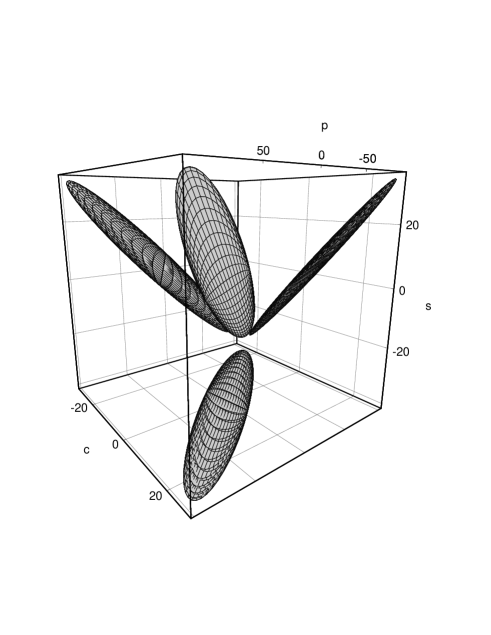
Figure 2: Possible combinations of point, slope and curvature at the end point $f^{+}(t_{-})$, allowed parameter triplets lie inside the ellipsoid. To clarify the position of the ellipsoid, it’s contours were drawn on three faces of the cube.

If one redefines $J(Q^{2})$ to include the residue and if one uses the analytic funtion $\tilde{f}$, (38) is the same as (34).

Since (34) is a sum of positive terms, we can cut off the sum at some value of $n$ and get (e.g. for $n\leq 2$)

$$[(\phi f)(0)]^{2}+[(\phi f)^{\prime}(0)]^{2}+\frac{1}{4}[(\phi f)^{\prime\prime}(0)]^{2}<J(Q^{2})$$ (39)

where we re–substituted $\psi$.

Such equations give us ellipsoids in the parameter space of value, slope and higher derivatives of the form factor at the kinematical end point, where all allowed parameter combinations lie inside the ellipsoid. If we take, for example, $n\leq 2$ as in (39) we would get a three–dimensional ellipsoid in point–slope–curvature–space (see figure 2).

The resulting constraints are not as good as the ones that can be obtained for $B\to D$ transitions [14, 15]; this is due to heavy quark symmetries, which are not as useful in $B\to\pi$ decays.

However, one may exploit the chiral symmetry for the light degrees of freedom as an additional physics input. These symmetries hold at small momenta of the pions and are therefore applicable in the end point region where the momentum transfer to the leptons becomes maximal. One may combine heavy quark and chiral symmetry as in [16]–[18] and compute the form factors in this limit. One finds [16]

$$f^{+}(t) = \frac{f_{B}}{2f_{\pi}}\left[1+\frac{g(M^{2}-m^{2}+t)}{M^{2}+m^{2}+2\Delta M-t}\right]$$

$$f^{0}(t) = \frac{f_{B}}{2f_{\pi}}\left[1+\frac{g(M^{2}-m^{2}+t)}{M^{2}+m^{2}+2\Delta M-t}\right.$$

$$\hskip 51.21504pt+\left.\frac{t}{M^{2}-m^{2}}\left\{1-\frac{g(3M^{2}-m^{2}+t)}{M^{2}+m^{2}+2\Delta M-t}\right\}\right]$$

which results in the residue

$$\mbox{Res}\{f,t_{p}\}=-\frac{f_{B}}{f_{\pi}}gM(M+\Delta)$$ (41)

at

$$t_{p}=M^{2}+m^{2}+2\Delta M$$ (42)

where $\Delta=m_{B^{*}}-m_{B}$. The additional parameters which appear in these relations are the chiral coupling constant $g$ which describes the $BB^{*}\pi$–coupling and the ratio of the decay constants $f_{B}/f_{\pi}$.

The form factors (3) are valid in the chiral limit, which holds only in a small piece of the kinmatically allowed region. In order to extend this to the full range, a variety of ansätze have been invented to extend this pole–behaviour to small $t$ (see e.g. [19]– [22]); however, this makes the extraction ov $V_{ub}$ model dependent.

We will now use the improved unitarity bounds and the chiral limit to derive bounds on the form factors. These bounds have the advantage to be model independent, however, as we shall see, they are not very tight over the whole range of $t$. This is mainly due to the fact that the parameters $g$ and $f_{B}/f_{\pi}$ suffer from large theoretical uncertainties.

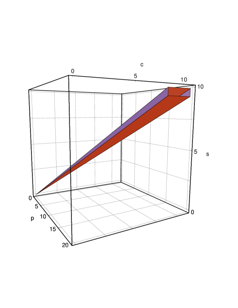
Figure 3: Possible combinations of point, slope and curvature at the end point $f^{+}(t_{-})$ using the chiral limit.

In the following we shall consider $f^{+}$ only; here we can avoid the problem of the large uncertainties in $g$ and $f_{B}/f_{\pi}$ by considering fractions like $f^{+\prime}(t_{-})/f^{+}(t_{-})$ and $f^{+\prime\prime}(t_{-})/f^{+}(t_{-})$ in which the $f_{B}/f_{\pi}$–dependence drops out and the remaining $g$–dependence is small, since terms involving $g$ are suppressed:

$$\frac{{f^{+}}^{\prime}(t_{-})}{f^{+}(t_{-})} = \frac{M+\Delta}{2M(M-m)(\Delta+m)}\frac{1}{1+\frac{\Delta+m}{g(M-m)}}\,,$$ (43)

$$\frac{{f^{+}}^{\prime\prime}(t_{-})}{f^{+}(t_{-})} = \frac{1}{2M^{2}(M-m)(\Delta+m)}\frac{1}{1+\frac{\Delta+m}{g(M-m)}}\,.$$ (44)

Thus in the chiral limit the ratios $f^{+\prime}(t_{-})/f^{+}(t_{-})$ and $f^{+\prime\prime}(t_{-})/f^{+}(t_{-})$ are practically fixed and we can express the slope $s$ and the curvature $c$ in terms of the value $p$ of $f^{+}$ at $t_{-}$. This would yield a straight line in a $p,s,c$ plot; however, varying the coupling $g$ in a generous range between $0.25$ and $0.5$ [23] and allowing for derivations of the chiral limit of about 15%, we obtain the rectangular cone shown in figure 3.

In case of the residue it is not possible to get rid of the $g$– and $f_{B}/f_{\pi}$–parameter, so one has to take the full uncertainties into account when calculating the bounds. One could also choose to drop the residue completely and work with the redefined $\phi_{p}(z,Q^{2})$ of (16) but we decided to use (41) because the resulting bounds are more stringent.

Using (3) and their first derivatives at the end point as input parameters in (3) (the extension to higher derivatives is trivial) we get upper and lower bounds for $0\leq t\leq t_{-}$ which depend strongly on the chiral parameters $g$ and $f_{B}/f_{\pi}$. In addition to that, a combination of figure 2 and 3 can be used to constrain the allowed range for the end point value of $f(t_{-})$ and its derivatives.

The combination of unitarity bounds, extended to include derivatives, and the chiral limit now allows us to calculate bounds for the form factors $f^{+}(t)$ and $f^{0}(t)$.

4 Numerical Results and Discussion

Inserting $t_{1}=t_{-}$ ($z_{1}=0$) in (3) one gets

$$\psi_{up,lo} = (\psi_{1}+\psi_{1}^{\prime}z)\pm\frac{z^{2}}{\sqrt{1-z^{2}}}\sqrt{J-\psi_{1}^{2}-[\psi_{1}^{\prime}]^{2}}$$ (45)

which leads to the bounds

$$F_{up,lo}=\frac{f_{1}\phi_{1}+(f_{1}\phi_{1})^{\prime}z}{\phi(z,Q^{2})}\pm\frac{z^{2}}{\phi(z,Q^{2})}\sqrt{\frac{J-(f_{1}\phi_{1})^{2}-[(f_{1}\phi_{1})^{\prime}]^{2}}{1-z^{2}}}.$$ (46)

We used $Q^{2}=0$ for the QCD calculations and inserted all possible combinations of end point value and slope into (46). We also allowed variation of $g$ and $f_{B}/f_{\pi}$ from $0.25\leq g\leq 0.5$ and $1\leq f_{B}/f_{\pi}\leq 1.7$ ([23, 24]). Within this variation we determined the bounds for fixed parameter values and finally took the loosest ones as our result.

We scanned the parameter space of possible $ps$–pairs by dividing the allowed $p$–range into small, equally spaced intervals. For each of these possible $p$–values, there exists an allowed $s$–range which is also divided into small intervalls. A similar procedure was applied for the chiral input parameters.

Figure 4: Bounds on the form factor $f^{+}(t)$, derived by using a fixed end point and varying the slope according to the chiral limit

Figure 4 shows the resulting bounds for the form factor $f^{+}$. The values of the form factor at $t_{-}$ vary between 3.2 and 13.5 due to the uncertainties in $f_{B}/f_{\pi}$ and $g$. The two solid lines represent the result for the maximal value of the form factor at $t_{-}$, where the upper (lower) line corresponds to the minimal (maximal) possible value for the slope at $t_{-}$. Similarly, we have plotted the corresponding lines for intermediate values of the form factor at $t_{-}$ down to the minimal value, represented by the long–dashed line.

The upper and lower bounds coincide at $t=0$ due to the kinematical constraint (2). We have computed $f^{0}$ in the same way as we did for $f^{+}$, scanning the parameter space for $p$ and $s$ at $t=t_{-}$. The resulting bounds for $f^{0}$ at $t=0$ are much tighter that those for $f^{+}(0)$ and hence the kinematical constraint has a significant effect on $f^{+}$. In order to be conservative we have varied the parameters for both form factors independently; that is we did not use the correlation between the form factors implied by the chiral limit, namely that at $t=t_{-}$ they are both given by the same two parameters $f_{B}/f_{\pi}$ and $g$.

In figure 5 we have combined the results for $f^{+}$ and $f^{0}$, plotting the upper bound for the maximal values of $f^{+}(t_{-})$ and $f^{0}(t_{-})$ with the minmal slopes and the lower bounds for the minmal values of $f^{+}(t_{-})$ and $f^{0}(t_{-})$ with the maximal slopes. Compared to the standard method (see figure 1) the inclusion of the slope and the chiral limit has significantly improved the bounds. We have to point out, however, that not any curve within these two bounds is allowed as a form factor, since QCD implies relations between slopes and the form factor values. This can be seen in figure 4.

Figure 5: Bounds on the form factors $f^{0}(t)$ (on the left side, $t$ increasing leftward) and $f^{+}(t)$ (on the right side, $t$ increasing rightward) derived with restriction on possible $ps$–pairs at $f(t_{-})$ and including the kinematical constraint, plotted over the whole kinematical range of $[0,t_{-}]$ ($t$ in $\mbox{GeV}^{2}$).

Finally one can also use model input into the machinery of unitarity bounds. In particular, a model can be used to obtain points and curvatures away from $t_{-}$.

In figure 6 and 7 we have used the ISGW II model [25] as an input. Fig.6 shows the bounds obtained by the standard formalism using two points ($t=10$ GeV² and $t_{-}$) from this model, while in fig.7 we use these two points but also the derivative at $t_{-}$, obtained again from ISGW II, as input parameters. The dashed line is the model prediction itself.

Another commonly used model is the BSW model [19]. In fig.8 we use this model to determine the value of the form factor $f^{+}$ at $t_{-}$, while in fig.9 also the slope at $t_{-}$ was taken from the model. It is interesting to note that if one also includes the curvature of $f^{+}$ at $t_{-}$ in the BSW model — as in fig.10 — the lower bound shifts significantly upwards, such that the model becomes inconsistent with the bounds. This indicates that the curvature of the BSW model is too large in the end point, since the lower bound comes out to be quite high; its value at $t=0$ is about one, which is in contradiction not only with the BSW model, but also with sum rule calculations [26, 27].

Figure 6: Bounds on $f^{0}$ (left) and $f^{+}$ (right) derived by using the ISGW II model and using the values at $t=10\mbox{ GeV}^{2}$ and $t=t_{-}$ as input parameters. The bounds are drawn solid, the dashed line corresponds to the model.

Figure 7: Same as in figure 6 but including the slope at $t=t_{-}$ as well.

Figure 8: Bounds on $f^{+}$ derived by using the BSW model and using the value at $t=t_{-}$ as input parameter. The bounds are drawn solid, the dashed line corresponds to the model.

Figure 9: Same as in figure 8 but including the slope at $t=t_{-}$ as well.

Figure 10: Same as in figure 9 but including the curvature at $t=t_{-}$ as well.

The pole form of the BSW model is motivated by the form factor in the chiral limit and thus it is no surprise that they have similar curvatures of $f^{+}$ at $t_{-}$. We take this as an indication that one should not exploit the chiral limit to obtain derivatives of the form factors beyond the slope; going beyond the slope requires to take into account higher orders in chiral perturabtion theory.

5 Conclusions

Using unitarity and analyticity to derive bounds on form factors using input from perturbative QCD has become a widely used tool, since this method allows to constrain form factors over the whole range of $q^{2}$ in a model independent way.

This method has attracted some attention in $B$ decays and has been combined with heavy quark symmetry; for the $b\to c$ transitions this has lead to stringent constraints on the form factors, i.e. the Isgur–Wise function.

In $B\to\pi$ transitions heavy quark symmetries are not as useful and it is necessary to obtain model independent information from other sources. The general bounds in $B\to\pi$ decays are not very tight and hence also not very useful. Including points where the form factor is known from other sources improves the bounds; this method has been combined with lattice data to obtain model independent bounds for the form factors for $B\to\pi$ transitions.

In the present paper we have focussed also at the $B\to\pi$ decays and improved the bounds on the relevant form factors one more step by including slopes and higher derivatives of form factors, which in some cases may be known from other sources. Again from unitarity the value, the slope, and even higher derivatives of the form factor at $t_{-}$ are constrained to lie inside an ellipsoid which can be used as an input into the machinery we have proposed here.

Still this does not tighten the bounds very much and some more physics input beyond perturbative QCD is needed. Close to the kinematical end point $t_{-}$ chiral perturbation theory is valid and we used the chiral limit of the form factors as an input. With this we arrived at bounds which are much tighter than the general bounds obtained without any knowledge on the form factors. The model independent results of our paper are shown in fig.4 and fig.5.

Finally one may also combine models with the unitarity bounds from QCD. Taking points, slopes and curvatures from these models one may test the consistency of a given model with QCD. An extensive analysis of the various models is beyond the scope of the present paper; we only considered the ISGW II and the BSW model as examples. Although both models lie within the bounds given in fig.5 (the ISGW II touching the lower bound at $t_{-}$), this still does not mean that they are consisten with QCD; the curvature of the BSW model at $t_{-}$ turns out to be incompatibel with the QCD constraints.

References

- [1] C. G. Boyd and I. Z. Rothstein, Phys. Lett. B420, 350 (1998), hep-ph/9711268.
- [2] S. Weinzierl and O. Yakovlev, (1997), hep-ph/9712399.
- [3] D. S. Hwang and B.-H. Lee, (1998), hep-ph/9801421.
- [4] A. Khodjamirian and R. Ruckl, (1998), hep-ph/9801443.
- [5] I. F. Shih and S. Okubo, Phys. Rev. D4, 3519 (1971).
- [6] S. Okubo, Phys. Rev. D3, 2807 (1971).
- [7] S. Okubo, Phys. Rev. D4, 725 (1971).
- [8] S. Okubo and I. F. Shih, Phys. Rev. D4, 2020 (1971).
- [9] C. Bourrely, B. Machet, and E. de Rafael, Nucl. Phys. B189, 157 (1981).
- [10] L. Lellouch, Nucl. Phys. B479, 353 (1996), hep-ph/9509358.
- [11] C. G. Boyd and M. J. Savage, Phys. Rev. D56, 303 (1997), hep-ph/9702300.
- [12] C. G. Boyd, B. Grinstein, and R. F. Lebed, Phys. Rev. D56, 6895 (1997), hep-ph/9705252.
- [13] J. G. Korner, D. Pirjol, and C. Dominguez, Phys. Lett. B301, 257 (1993).
- [14] I. Caprini and M. Neubert, Phys. Lett. B380, 376 (1996), hep-ph/9603414.
- [15] I. Caprini, L. Lellouch, and M. Neubert, (1997), hep-ph/9712417.
- [16] M. B. Wise, Phys. Rev. D45, 2188 (1992).
- [17] G. Burdman and J. Kambor, Phys. Rev. D55, 2817 (1997), hep-ph/9602353.
- [18] G. Burdman, (1997), hep-ph/9707410.
- [19] M. Wirbel, B. Stech, and M. Bauer, Z. Phys. C29, 637 (1985).
- [20] B. Grinstein and P. F. Mende, Nucl. Phys. B425, 451 (1994), hep-ph/9401303.
- [21] J. G. Korner, K. Schilcher, M. Wirbel, and Y. L. Wu, Z. Phys. C48, 663 (1990).
- [22] G. Burdman and J. F. Donoghue, Phys. Rev. Lett. 68, 2887 (1992).
- [23] R. Casalbuoni et al., Phys. Rept. 281, 145 (1997), hep-ph/9605342.
- [24] J. M. Flynn and C. T. Sachrajda, (1997), hep-lat/9710057.
- [25] D. Scora and N. Isgur, Phys. Rev. D52, 2783 (1995), hep-ph/9503486.
- [26] V. M. Belyaev, A. Khodjamirian, and R. Ruckl, Z. Phys. C60, 349 (1993), hep-ph/9305348.
- [27] P. Ball, (1998), hep-ph/9802394.