CERN–TH/98–162 NORDITA–98–41–HE hep-ph/9805422

Exclusive Semileptonic and Rare B-Meson Decays
in QCD
Patricia Ball^1,, V.M. Braun^2,

¹ CERN–TH, CH–1211 Genève 23, Switzerland

²NORDITA, Blegdamsvej 17, DK–2100 Copenhagen, Denmark

Abstract:
We present the first complete results for the semileptonic and rare radiative form factors of $B$-mesons weak decay into a light vector-meson ($\rho,\omega,K^{*},\phi$) in the light-cone sum-rule approach. The calculation includes radiative corrections, higher-twist corrections and SU(3)-breaking effects. The theoretical uncertainty is investigated in detail. A simple parametrization of the form factors is given in terms of three parameters each. We find that the form factors observe several relations inspired by heavy-quark symmetry.
Submitted to Physical Review D

1 Introduction

The challenge to understand the physics of CP-violation related to the structure of the CKM mixing matrix in (and beyond) the Standard Model is fuelling an impressive experimental programme for the study of $B$-decays, both exclusive and inclusive. Abundant data in various exclusive channels are expected to arrive within the next few years from the dedicated $B$-factories BaBar and Belle; their potential impact on our understanding of CP-violation at the electroweak scale will crucially depend on our possibility to control the effects of strong interactions. For exclusive decays with only one hadron in the final state, the task is to calculate various transition form factors; it has already attracted significant attention in the literature.

In this paper we present the first complete results for the exclusive semileptonic and rare radiative $B$-decays to light vector-mesons in the light-cone sum-rule approach. Exclusive decays, which are the principal concern of this work, can be grouped as semileptonic decays:

• $B_{u,d}\to\rho e\nu$,

• $B_{s}\to K^{*}e\nu$,

rare decays corresponding to $b\to s$ transitions, which we term CKM-allowed:

• $B_{u,d}\to K^{*}+\gamma$,     $B_{u,d}\to K^{*}+l^{+}l^{-}$,

• $B_{s}\to\phi+\gamma$,     $B_{s}\to\phi+l^{+}l^{-}$,

and $b\to d$ transitions, which we call CKM-suppressed:

• $B_{d}\to(\rho,\omega)+\gamma$,     $B_{d}\to(\rho,\omega)+l^{+}l^{-}$,

• $B_{u}\to\rho+\gamma$,     $B_{u}\to\rho+l^{+}l^{-}$,

• $B_{s}\to K^{*}+\gamma$,     $B_{s}\to K^{*}+l^{+}l^{-}$.

Let $V$ be a vector-meson, i.e. $\rho$, $\omega$, $K^{*}$ or $\phi$, and let $p_{\mu}$, $\epsilon^{*}_{\mu}$ and $m_{V}$ be its momentum, polarization vector and mass, respectively. Let $p_{B}$ ($m_{B}$) be the momentum (mass) of the $B$-meson. We define semileptonic form factors by ($q=p_{B}-p$)

$$\langle V(p)|(V-A)_{\mu}|B(p_{B})\rangle = -i\epsilon^{*}_{\mu}(m_{B}+m_{V})A_{1}^{V}(q^{2})+i(p_{B}+p)_{\mu}(\epsilon^{*}p_{B})\,\frac{A_{2}^{V}(q^{2})}{m_{B}+m_{V}}$$

$$+\>iq_{\mu}(\epsilon^{*}p_{B})\,\frac{2m_{V}}{q^{2}}\,\left(A_{3}^{V}(q^{2})-A_{0}^{V}(q^{2})\right)+\epsilon_{\mu\nu\rho\sigma}\epsilon^{*\nu}p_{B}^{\rho}p^{\sigma}\,\frac{2V^{V}(q^{2})}{m_{B}+m_{V}}\,.$$ (1.1)

Note the exact relations

$$A_{3}^{V}(q^{2}) = \frac{m_{B}+m_{V}}{2m_{V}}\,A_{1}^{V}(q^{2})-\frac{m_{B}-m_{V}}{2m_{V}}\,A_{2}^{V}(q^{2}),$$

$$A_{0}^{V}(0) = A_{3}^{V}(0),$$

$$\langle V|\partial_{\mu}A^{\mu}|B\rangle = 2m_{V}(\epsilon^{*}p_{B})A_{0}^{V}(q^{2}).$$ (1.2)

The second relation in (1.2) ensures that there is no kinematical singularity in the matrix element at $q^{2}=0$.

Rare decays are described by the above semileptonic form factors and the following penguin form factors:

$$\langle V|\bar{\psi}\sigma_{\mu\nu}q^{\nu}(1+\gamma_{5})b|B(p_{B})\rangle = i\epsilon_{\mu\nu\rho\sigma}\epsilon^{*\nu}p_{B}^{\rho}p^{\sigma}\,2T_{1}(q^{2})$$ (1.3)

$${}+T_{2}(q^{2})\left\{\epsilon^{*}_{\mu}(m_{B}^{2}-m_{V}^{2})-(\epsilon^{*}p_{B})\,(p_{B}+p)_{\mu}\right\}$$

$${}+T_{3}(q^{2})(\epsilon^{*}p_{B})\left\{q_{\mu}-\frac{q^{2}}{m_{B}^{2}-m_{V}^{2}}\,(p_{B}+p)_{\mu}\right\}$$

with

$$T_{1}(0)=T_{2}(0).$$ (1.4)

Here $\psi=s,d$. All signs are defined in such a way as to render the form factors positive.

The physical range of $q^{2}$ extends from $q^{2}_{\rm min}=0$ to $q^{2}_{\rm max}=(m_{B}-m_{V})^{2}$ for three-body decays and $q^{2}\equiv 0$ for two-body decays.

The method of light-cone sum-rules was first suggested for the study of weak baryon-decays in [1] and later extended to heavy-meson decays in [2]. It is a non-perturbative approach, which combines ideas of QCD sum-rules [3] with the twist-expansion characteristic of hard exclusive processes in QCD [4] and makes explicit use of the large energy of the final-state vector-meson at small values of the momentum-transfer to leptons, $q^{2}$. In this respect, the light-cone sum-rule approach is complementary to lattice calculations [5], which are mainly restricted to form factors at small recoil (large values of $q^{2}$). Of course, the light-cone sum-rules lack the rigour of the lattice approach. Nevertheless, they prove to provide a powerful non-perturbative model, which is explicitly consistent with perturbative QCD and the heavy-quark limit.

Early studies of exclusive $B$-decays in the light-cone sum-rule approach were restricted to contributions of leading-twist and did not take radiative corrections into account, see Refs. [6, 7] for a review and references to original publications. Very recently, these corrections have been calculated for the semileptonic $B\to\pi,Ke\nu$ decays [8]. In this work we calculate radiative and higher-twist corrections to all form factors involving vector-mesons (see above) making use of new results on distribution amplitudes of vector-mesons, reported in [9, 10, 11]. We find that the corrections in question are fairly small in all cases.

The presentation is organized as follows: in Sec. 2 we recall basic ideas of the light-cone sum-rule approach and derive radiative and higher-twist corrections to the form factors in question in a compact form. Section 3 presents our main results and includes a discussion of input-parameters as well as error estimates. In Sec. 4 we discuss relations between semileptonic and penguin form factors in the heavy-quark limit. Section 5 is reserved to a summary and conclusions. The paper has two appendices: in App. A we collect the relevant loop integrals for the calculation of radiative corrections. Appendix B contains a summary of the results of [9, 10, 11] on vector-meson distribution amplitudes.

2 Method and Calculation

2.1 General Framework

Consider semileptonic $B_{d}\to\rho e\nu$ and rare $B_{d}\to K^{*}\ell^{+}\ell^{-}$ decays as representative examples. We choose a $B$-meson “interpolating current” $j_{B}=\bar{d}i\gamma_{5}b$, so that

$$\langle 0|j_{B}|B(p_{B})\rangle=\frac{f_{B}m_{B}^{2}}{m_{b}}\,,$$ (2.1)

where $f_{B}$ is the usual $B$-decay constant and $m_{b}$ the $b$-quark mass. In order to obtain information on the form factors, we study the set of suitable correlation functions:

$$i\int d^{4}ye^{-ip_{B}y}\langle\rho(p)|T(V-A)_{\mu}(0)j_{B}^{\dagger}(y)|0\rangle\ =\ -i\Gamma^{0}(p_{B}^{2},q^{2})\epsilon^{*}_{\mu}$$ (2.2)

$${}+i\Gamma^{+}(p_{B}^{2},q^{2})\,\frac{\epsilon^{*}q}{pq}\,(q+2p)_{\mu}+i\Gamma^{-}(p_{B}^{2},q^{2})\,\frac{\epsilon^{*}q}{pq}\,q_{\mu}+\Gamma^{V}(p_{B}^{2},q^{2})\epsilon_{\mu}^{\phantom{\mu}\alpha\beta\gamma}\epsilon^{*}_{\alpha}q_{\beta}p_{\gamma},$$

$$i\int d^{4}ye^{-ip_{B}y}\langle K^{*}(p)|T[\bar{s}\sigma_{\mu\nu}\gamma_{5}b](0)j_{B}^{\dagger}(y)|0\rangle\ =\ {\cal A}(p_{B}^{2},q^{2})\{\epsilon^{*}_{\mu}(2p+q)_{\nu}-\epsilon^{*}_{\nu}(2p+q)_{\mu}\}$$ (2.3)

$${}-{\cal B}(p_{B}^{2},q^{2})\{\epsilon^{*}_{\mu}q_{\nu}-\epsilon^{*}_{\nu}q_{\mu})\}-2{\cal C}(p_{B}^{2},q^{2})\,\frac{\epsilon^{*}q}{pq}\,\{p_{\mu}q_{\nu}-q_{\mu}p_{\nu}\}.$$

The Lorentz-invariant functions $\Gamma^{0,\pm,V},{\cal A},{\cal B},{\cal C}$ can be calculated in QCD for large Euclidian $p_{B}^{2}$. More precisely, if $m_{b}^{2}-p_{B}^{2}\ll 0$, then the correlation functions (2.2), (2.3) are dominated by the region of small $y^{2}$ and can be systematically expanded in powers of the deviation from the light-cone $y^{2}=0$. The light-cone expansion presents a modification of the usual Wilson operator product expansion, such that relevant operators are non-local and are classified in terms of twist rather than dimension. Matrix elements of non-local light-cone operators between the vacuum and the vector-meson state define meson distribution amplitudes [4], which describe the partition of the meson-momentum between the constituents in the infinite momentum frame. In particular, there exist two leading-twist distribution amplitudes for vector-mesons, see App. B, corresponding to longitudinal and transverse polarizations, respectively:

$$\langle\rho|\bar{u}(0)\gamma_{\mu}d(z)|0\rangle = f_{\rho}m_{\rho}p_{\mu}\,\frac{\epsilon^{*}z}{pz}\,\int_{0}^{1}\!\!du\,e^{i\bar{u}pz}\,\phi_{\parallel}(u,\mu),$$ (2.4)

$$\langle\rho|\bar{u}(0)\sigma_{\mu\nu}d(z)|0\rangle = -if_{\rho}^{T}(\mu)(\epsilon^{*}_{\mu}p_{\nu}-p_{\mu}\epsilon^{*}_{\nu})\int_{0}^{1}\!\!du\,e^{i\bar{u}pz}\,\phi_{\perp}(u,\mu),$$ (2.5)

and similarly for $K^{*}$ and $\phi$. Here $z$ is an auxiliary light-like vector, $u$ is the momentum fraction carried by the valence quark, and the decay constants $f_{\rho}$, $f_{\rho}^{T}$ are defined in App. B, while $\mu$ specifies the scale: extraction of the leading asymptotic behaviour in field theories invariably produces singularities, which reflect themselves in the scale dependence of distribution amplitudes. As always, this scale dependence cancels in physical quantities by a corresponding dependence of coefficient functions.

The invariant amplitudes in (2.2), (2.3) can be calculated in terms of meson distribution amplitudes, in complete analogy with the calculation of structure functions in deep inelastic lepton-nucleon scattering in terms of nucleon parton-distributions: the off-shellness $m_{b}^{2}-p_{B}^{2}$ plays the role of photon virtuality $Q^{2}$. As an illustration, consider the tree-level leading-twist result for $\Gamma^{0}$, adapted from Ref. [12]:

$$\Gamma^{0}(p_{B}^{2},q^{2})=\int_{0}^{1}\!\!du\,\frac{1}{m_{b}^{2}-up_{B}^{2}-\bar{u}q^{2}}\,f^{T}_{V}\phi_{\perp}(u)\,\frac{m_{b}^{2}-q^{2}}{2u}.$$ (2.6)

We want to emphasize that the procedure is rigorous at this point: all corrections can (in principle) be included in a systematic way, and their evaluation is precisely the subject of this work.

The subtle part concerns the extraction of the $B$-meson contribution to the invariant amplitudes. The exact amplitude $\Gamma^{0}$ (in nature) has a pole at $p_{B}^{2}=m_{B}^{2}$ corresponding to the intermediate $B$-meson state, and this contribution can be written in terms of the form factor $A_{1}^{B\to\rho}$ defined in (1.1):

$$\Gamma^{0}_{B\mbox{-meson}}=(m_{B}+m_{\rho})A_{1}^{B\to\rho}(q^{2})\cdot\frac{1}{m^{2}_{B}-p_{B}^{2}}\cdot\frac{m_{B}^{2}f_{B}}{m_{b}}\,.$$ (2.7)

On the other hand, the QCD calculation at $p_{B}^{2}\ll m_{b}^{2}$ is only approximate and, continued analytically to “Minkowskian” $p_{B}^{2}>m_{b}^{2}$, produces a smooth imaginary part with no sign of a pole behaviour. To proceed, we invoke the concept of duality, assuming that the exact spectral density and the one calculated in QCD coincide on the average, that is integrated over a sufficient region of energy. In particular, we assume that the $B$-meson contribution is obtained by the integral of the QCD spectral density over the duality region:

$$\Gamma^{0}_{B\mbox{-meson}}=\frac{1}{2\pi i}\int\limits_{m_{b}^{2}}^{s_{0}}\frac{ds}{s-p_{B}^{2}}\,{\rm Disc\,}_{p_{B}^{2}}\Gamma^{0}_{\rm QCD}(s,q^{2}).$$ (2.8)

The parameter $s_{0}\approx(34$–$35)$ GeV² is called “continuum-threshold” and is fixed from QCD sum-rules for $f_{B}$, see e.g. [13]. Equating the above two representations, one obtains a light-cone sum-rule for the form factor $A_{1}$. Sum-rules for the other form factors are constructed in precisely the same manner.

While the accuracy of the QCD calculation can be controlled (and improved), the duality approximation introduces an irreducible uncertainty in predictions for the form factors, which is usually believed to be of order (10–15)%. Practical calculations in the sum-rule framework involve some technical tricks to reduce this uncertainty, e.g. Borel transformation, which we will not discuss here. These techniques are well established and their detailed description in the particular context of light-cone sum-rules can be found, for instance, in Refs. [7, 12]. The work [12] also contains a detailed comparison of the light-cone sum-rule approach to traditional QCD sum-rules and can serve as introduction for the more theoretically-minded reader.

2.2 Radiative Corrections

Radiative corrections to the sum-rules correspond to one-loop corrections to the coefficient functions in front of leading-twist distribution amplitudes and are given by the diagrams shown in Fig. 1.

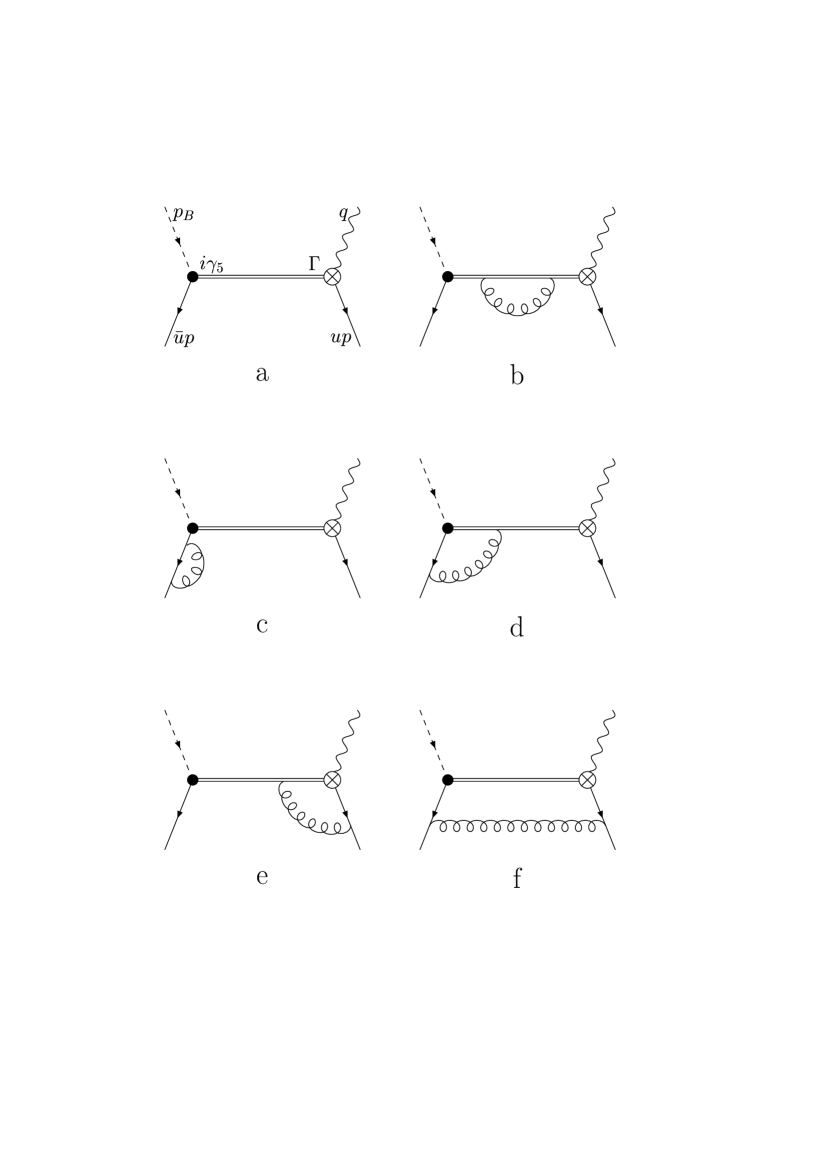
Figure 1: The leading-order diagram (a) and one-loop radiative corrections (b–f).

The calculation is done in dimensional regularization, and it is sufficient to consider matrix elements over on-shell massless quark and antiquark carrying momentum fraction $up$ and $\bar{u}p$, respectively. The transversely polarized and longitudinally polarized meson states are projected on by

$$\langle V_{\perp}(p)|\bar{u}_{a}(0)d_{b}(x)|0\rangle = -\frac{i}{4}\,f_{V}^{T}[\sigma_{\mu\nu}]_{ba}\epsilon^{*\mu}p^{\nu}\int du\,e^{i\bar{u}px}\phi_{\perp}(u)$$ (2.9)

$$\equiv -\frac{1}{8}\,f_{V}^{T}[\sigma^{\mu\nu}\gamma_{5}]_{ba}\epsilon_{\mu\nu\rho\sigma}\epsilon^{*\rho}p^{\sigma}\int du\,e^{i\bar{u}px}\phi_{\perp}(u),$$ (2.10)

$$\langle V_{\parallel}(p)|\bar{u}_{a}(0)d_{b}(x)|0\rangle \equiv \frac{1}{4}\,f_{V}m_{V}[{\mathchoice{\c@ncel\displaystyle{p}}{\c@ncel\textstyle{p}}{\c@ncel\scriptstyle{p}}{\c@ncel\scriptscriptstyle{p}}}]_{ba}\,\frac{\epsilon^{*}x}{px}\,\int du\,e^{i\bar{u}px}\phi_{\parallel}(u)$$ (2.11)

$${}\stackrel{{\scriptstyle m_{V}^{2}\to 0}}{{\longrightarrow}}\frac{1}{4}\,f_{V}[{\mathchoice{\c@ncel\displaystyle{p}}{\c@ncel\textstyle{p}}{\c@ncel\scriptstyle{p}}{\c@ncel\scriptscriptstyle{p}}}]_{ba}\int du\,e^{i\bar{u}px}\phi_{\parallel}(u),$$

where $a,b$ are spinor indices. In the last line in (2.11) we made use of the fact that for ultrarelativistic longitudinal vector-mesons $\epsilon_{\mu}\to p_{\mu}/m_{V}$ up to $O(m_{V}^{2}/|\vec{p}|^{2})$ corrections. This is a justified approximation for the calculation of radiative corrections to leading-twist accuracy, to which end the meson-mass can be neglected throughout. For further use we introduce the notation for the projection operators:

$${\cal P}_{\parallel} = \frac{1}{4}f_{V}{\mathchoice{\c@ncel\displaystyle{p}}{\c@ncel\textstyle{p}}{\c@ncel\scriptstyle{p}}{\c@ncel\scriptscriptstyle{p}}},$$

$${\cal P}_{\perp} = -\frac{i}{4}f_{V}^{T}\sigma_{\alpha\beta}\epsilon^{*\alpha}p^{\beta}\quad{\rm\ or\ }\quad{\cal P}_{\perp}^{(5)}=-\frac{1}{8}f_{V}^{T}\sigma_{\alpha\beta}\gamma_{5}\epsilon^{\alpha\beta\rho\sigma}\epsilon^{*}_{\rho}p_{\sigma}.$$ (2.12)

In what follows, they will be treated as $D$-dimensional objects .

The calculation in question is in principle straightforward and similar to the existing calculations of NLO corrections to hard exclusive processes [14]. One has to consider one-loop diagrams with a heavy-quark and two different kinematic invariants $q^{2}$ and $p_{B}^{2}$, which makes formulas rather cumbersome. The specific requirement is to organize the expressions in a form suitable for a dispersion representation in $p_{B}^{2}$, cf. Eq. (2.8), so that continuum subtraction can be made.

Analytic expressions for $B$-decays to light pseudoscalar-mesons $\pi,K$ have been made available recently [8]. For vector-mesons the number of form factors is so large that working out (relatively) compact analytic expressions is not worth the effort. In this work we prefer to give the formulae in terms of traces and general momentum integrals (see below and App. A), which can be compiled and evaluated numerically using the mathematica programming language.

A usual subtlety concerns the treatment of $\gamma_{5}$. The results for the form factors given below are obtained using “naive dimensional regularization” (NDR), and the same scheme has to be applied to the calculation of Wilson coefficients for penguin operators.

There are two form factors in whose calculation one encounters an odd number of $\gamma_{5}$ in traces, which could cause ambiguities: $V$ and $T_{1}$. Only transverse mesons contribute to these form factors. In both cases, a possible ambiguity comes solely from the $B$-vertex correction in Fig. 1d, whereas in all other diagrams contraction of $\gamma$ matrices over $\gamma_{5}$ can be avoided. There are several ways out: (a) use a ’t Hooft-Veltman prescription for $\gamma_{5}$ and apply a finite renormalization to restore the Ward identities, as in [15]; (b) instead of the “natural” projection (2.9), use (2.10), which introduces a second $\gamma_{5}$ and thus eliminates the problem; (c) modify the definition of the form factors (1.3) to

$$\langle V|\bar{s}\sigma_{\mu\nu}\gamma_{5}b|B\rangle = A(q^{2})\left\{\epsilon^{*}_{\mu}(p_{B}+p)_{\nu}-(p_{B}+p)_{\mu}\epsilon^{*}_{\nu}\right\}-B(q^{2})\left\{\epsilon^{*}_{\mu}q_{\nu}-q_{\mu}\epsilon^{*}_{\nu}\right\}$$ (2.13)

$${}-C(q^{2})\,\frac{\epsilon^{*}p_{B}}{m_{B}^{2}-m_{V}^{2}}\,\left\{(p_{B}+p)_{\mu}q_{\nu}-q_{\mu}(p_{B}+p)_{\nu}\right\}.$$

Using

$$\sigma_{\mu\nu}\gamma_{5}=-\frac{i}{2}\,\epsilon_{\mu\nu\rho\sigma}\,\sigma^{\rho\sigma}$$

and contracting with $q^{\nu}$, one finds

$$A(q^{2}) = T_{1}(q^{2}),$$

$$B(q^{2}) = \frac{m_{B}^{2}-m_{V}^{2}}{q^{2}}\left[T_{1}(q^{2})-T_{2}(q^{2})\right],$$

$$C(q^{2}) = T_{3}(q^{2})-\frac{m_{B}^{2}-m_{V}^{2}}{q^{2}}\left[T_{1}(q^{2})-T_{2}(q^{2})\right],$$ (2.14)

from which the relation (1.4) follows. It is thus sufficient to calculate $A$, $B$ and $C$ instead of $T_{i}$ with the premium to avoid any $\gamma_{5}$ problem. We have checked that all of the above prescriptions yield identical results.

After these preliminary remarks, we are now in a position to calculate the diagrams in Fig. 1. The tree-level contribution of Fig. 1a equals

$$T^{(0)}=\frac{i}{s}\,{\rm Tr}(\Gamma({\mathchoice{\c@ncel\displaystyle{p}}{\c@ncel\textstyle{p}}{\c@ncel\scriptstyle{p}}{\c@ncel\scriptscriptstyle{p}}}_{B}-\bar{u}{\mathchoice{\c@ncel\displaystyle{p}}{\c@ncel\textstyle{p}}{\c@ncel\scriptstyle{p}}{\c@ncel\scriptscriptstyle{p}}}+m_{b})\gamma_{5}{\cal P}),$$ (2.15)

where $\Gamma$ is the Dirac structure of the weak vertex, ${\cal P}$ is one of the projection operators defined in Eqs. (2.12), and

$$s=m_{b}^{2}-up_{B}^{2}-\bar{u}q^{2}.$$

It proves convenient to replace in Eq. (2.15) the running $\overline{\rm MS}$ $b$-quark mass by the one-loop pole mass, which is given by

$$m_{\rm pole}=m_{\overline{\rm MS}}\left\{1+C_{F}\,\frac{g^{2}}{4\pi^{2}}\left(1-\frac{3}{4}\,\ln\,\frac{m^{2}}{\mu^{2}}\right)\right\}.$$ (2.16)

This replacement induces the radiative correction

$$T^{\rm pole} = 2i\,\frac{m_{b}^{2}}{s^{2}}\,C_{F}\,\frac{g^{2}}{4\pi^{2}}\,\left(1-\frac{3}{4}\,\ln\,\frac{m_{b}^{2}}{\mu^{2}}\right){\rm Tr}({\cal P}\Gamma({\mathchoice{\c@ncel\displaystyle{p}}{\c@ncel\textstyle{p}}{\c@ncel\scriptstyle{p}}{\c@ncel\scriptscriptstyle{p}}}_{B}-\bar{u}{\mathchoice{\c@ncel\displaystyle{p}}{\c@ncel\textstyle{p}}{\c@ncel\scriptstyle{p}}{\c@ncel\scriptscriptstyle{p}}}+m_{b})\gamma_{5})$$ (2.17)

$${}-\frac{i}{s}\,m_{b}C_{F}\,\frac{g^{2}}{4\pi^{2}}\left(1-\frac{3}{4}\,\ln\,\frac{m_{b}^{2}}{\mu^{2}}\right){\rm Tr}({\cal P}\Gamma({\mathchoice{\c@ncel\displaystyle{p}}{\c@ncel\textstyle{p}}{\c@ncel\scriptstyle{p}}{\c@ncel\scriptscriptstyle{p}}}_{B}-\bar{u}{\mathchoice{\c@ncel\displaystyle{p}}{\c@ncel\textstyle{p}}{\c@ncel\scriptstyle{p}}{\c@ncel\scriptscriptstyle{p}}})\gamma_{5}).$$

The general strategy is to simplify the traces as much as possible, but to keep ${\cal P}$ and $\Gamma$ arbitrary. Also contraction of $\gamma$ matrices over $\gamma_{5}$ is only allowed in the $B$-vertex correction.

It turns out that all one-loop diagrams can be expressed in terms of the following traces:

$$\,{\rm Tr}_{1} = {\rm Tr}\left({\cal P}\Gamma{\mathchoice{\c@ncel\displaystyle{q}}{\c@ncel\textstyle{q}}{\c@ncel\scriptstyle{q}}{\c@ncel\scriptscriptstyle{q}}}\gamma_{5}\right)\equiv{\rm Tr}\left({\cal P}\Gamma{\mathchoice{\c@ncel\displaystyle{p}}{\c@ncel\textstyle{p}}{\c@ncel\scriptstyle{p}}{\c@ncel\scriptscriptstyle{p}}}_{B}\gamma_{5}\right),$$

$$\,{\rm Tr}_{2} = {\rm Tr}\left({\cal P}\Gamma\gamma_{5}\right),$$

$$\,{\rm Tr}_{3} = {\rm Tr}\left({\cal P}{\mathchoice{\c@ncel\displaystyle{q}}{\c@ncel\textstyle{q}}{\c@ncel\scriptstyle{q}}{\c@ncel\scriptscriptstyle{q}}}\Gamma\gamma_{5}\right)\equiv{\rm Tr}\left({\cal P}{\mathchoice{\c@ncel\displaystyle{p}}{\c@ncel\textstyle{p}}{\c@ncel\scriptstyle{p}}{\c@ncel\scriptscriptstyle{p}}}_{B}\Gamma\gamma_{5}\right),$$

$$\,{\rm Tr}_{4} = {\rm Tr}({\cal P}{\mathchoice{\c@ncel\displaystyle{q}}{\c@ncel\textstyle{q}}{\c@ncel\scriptstyle{q}}{\c@ncel\scriptscriptstyle{q}}}\Gamma{\mathchoice{\c@ncel\displaystyle{q}}{\c@ncel\textstyle{q}}{\c@ncel\scriptstyle{q}}{\c@ncel\scriptscriptstyle{q}}}\gamma_{5}).$$ (2.18)

Let us also introduce

$$a_{\cal P}{\cal P}:=\gamma_{\alpha}{\cal P}\gamma^{\alpha},\qquad a_{\Gamma}\Gamma:=\gamma_{\alpha}\Gamma\gamma^{\alpha}.$$ (2.19)

The $b$-quark self-energy diagram in Fig. 1b is:

$$T^{\rm SE}_{b} = -\frac{g^{2}C_{F}}{s^{2}}\,\left\{\left[4m_{b}^{2}\left(Y+(1-\epsilon)Z\right)+2s(1-\epsilon)(Y-Z)\right](\,{\rm Tr}_{1}+m_{b}\,{\rm Tr}_{2})\right.$$ (2.20)

$$\left.-2m_{b}s\left(Y+(1-\epsilon)Z\right)\,{\rm Tr}_{2}\right\},$$

where $D=4-2\epsilon$ and the expressions for momentum integrals $Y,Z$ are given in App. A. The self-energy insertions in external light-quark legs in Fig. 1c only contribute logarithmic terms in dimensional regularization:

$$T^{\rm SE}_{l}=\frac{g^{2}C_{F}}{s}\left({\rm Tr}_{1}+m_{b}{\rm Tr}_{2}\right)\left(\ln\frac{m_{b}^{2}}{\mu_{UV}^{2}}-\ln\frac{m_{b}^{2}}{\mu_{IR}^{2}}\right),$$ (2.21)

where we distinguish between the ultra-violet scale $\mu_{UV}$, which is to be identified with the renormalization scale of the curent $j_{B}$ and the penguin operators, and the infra-red renormalization-scale $\mu_{IR}$ corresponding to the factorization scale in meson distribution amplitudes.

For the $B$-vertex correction in Fig. 1d, one obtains:

$$T^{B}=2\,\frac{g^{2}C_{F}}{s}\left\{\left(-8\bar{C}(1-\epsilon)-1-m_{b}^{2}\bar{B}+\bar{u}(p_{B}^{2}-q^{2})\bar{A}\right)(\,{\rm Tr}_{1}+m_{b}\,{\rm Tr}_{2})-m_{b}s\bar{B}\,{\rm Tr}_{2}\right\}.$$ (2.22)

For the weak vertex in Fig. 1e we find:

$$T^{W} = {}-\frac{g^{2}C_{F}}{s}\left\{a_{\Gamma}^{2}\,C\,(\,{\rm Tr}_{1}+m_{b}\,{\rm Tr}_{2})+a_{\Gamma}\,D\,(q^{2}\,{\rm Tr}_{3}+m_{b}\,{\rm Tr}_{4})+(p_{B}^{2}-q^{2})ua_{\Gamma}\,E\,{\rm Tr}_{3}\right.$$

$$\left.+2(p_{B}^{2}-q^{2})uA(\,{\rm Tr}_{1}+m_{b}\,{\rm Tr}_{2})+m_{b}B\left[2(m_{b}\,{\rm Tr}_{1}+q^{2}\,{\rm Tr}_{2})-a_{\Gamma}(m_{b}\,{\rm Tr}_{3}+\,{\rm Tr}_{4})\right]\right\}.$$ (2.23)

Finally, the box-diagram in Fig. 1f can be written as

$$T^{\rm box}=-g^{2}C_{F}a_{\cal P}\left\{a_{\cal P}H(\,{\rm Tr}_{1}+m_{b}\,{\rm Tr}_{2})+I(-m_{b}\,{\rm Tr}_{4}+(s-m_{b}^{2})\,{\rm Tr}_{3})+{B}_{u=1}\,{\rm Tr}_{3}\right\},$$ (2.24)

where ${B}_{u=1}$ is the limiting value of $B$ for $u\to 1$.

Definitions and explicit expressions for the one-loop integrals $A$, $B$, $C$, etc., are given in App. A.

2.3 Higher-Twist Contributions

Higher-twist terms generically refer to contributions to the light-cone expansion of the correlation functions (2.2) and (2.3), which are suppressed by powers of $1/(m_{b}^{2}-p_{B}^{2})$. In the sum-rules, such corrections are suppressed by powers of the Borel parameter. Higher-twist corrections are usually divided into “kinematical”, originating from the non-zero mass of the vector-meson, and “dynamical”, related to contributions of higher Fock-states and transverse quark-motion. In this paper we take into account both effects to twist-4 accuracy, making use of the new results on distribution amplitudes of vector-mesons reported in [10, 11] and summarized in App. B.

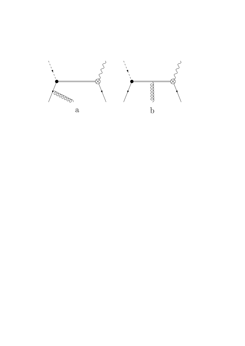
Figure 2: The higher-twist contributions.

The calculation is most conveniently done using the background-field approach of [16]. The diagrams of the type shown in Fig. 2a are taken into account within this method by the expansion of the non-local quark-antiquark operator in powers of the deviation from the light-cone; they give rise to contributions of two-particle distribution amplitudes of higher-twist, see Eqs. (B.12) and (B.27). The contribution of the gluon-emission from the heavy-quark is calculated using the light-cone expansion of the quark-propagator [16, 17]:

$$\langle 0|T\{b(x)\bar{b}(0)\}|0\rangle\ =$$ (2.25)

$$= {}iS_{b}(x)-ig\int\!\!\frac{d^{4}k}{(2\pi)^{4}}\,e^{-ikx}\!\!\int_{0}^{1}\!\!dv\left[\frac{1}{2}\,\frac{{\mathchoice{\c@ncel\displaystyle{k}}{\c@ncel\textstyle{k}}{\c@ncel\scriptstyle{k}}{\c@ncel\scriptscriptstyle{k}}}+m_{b}}{(m_{b}^{2}-k^{2})^{2}}\,G^{\mu\nu}(vx)\sigma_{\mu\nu}+\frac{v}{m_{b}^{2}-k^{2}}\,x_{\mu}G^{\mu\nu}(vx)\gamma_{\nu}\right]\!,\makebox[22.76219pt]{\ }$$

where $S_{b}(x)$ is the free quark-propagator. As in the case of radiative corrections, our strategy in this work is to derive the most general expression for all form factors in question, suitable for implementation in analytic/numerical calculations using mathematica. We obtain

$${\rm CF} = \frac{1}{4}\int_{0}^{1}\!\!du\left\{if_{V}m_{V}\left[\left(\Phi_{\parallel}^{(i)}(u)\epsilon^{*}_{\alpha}\,\frac{\partial}{\partial Q_{\alpha}}+\frac{\epsilon^{*}q}{pq}\,\frac{1}{16}\,m_{V}^{2}{\mathbb{A}}(u)\,\frac{\partial^{2}}{\partial Q_{\rho}\partial Q^{\rho}}\right)Tr(\Gamma S_{b}(Q)\gamma_{5}{\mathchoice{\c@ncel\displaystyle{p}}{\c@ncel\textstyle{p}}{\c@ncel\scriptstyle{p}}{\c@ncel\scriptscriptstyle{p}}})\right.\right.$$ (2.26)

$${}-g_{\perp}^{(v)}(u)Tr(\Gamma S_{b}(Q)\gamma_{5}{\mathchoice{\c@ncel\displaystyle{\epsilon}}{\c@ncel\textstyle{\epsilon}}{\c@ncel\scriptstyle{\epsilon}}{\c@ncel\scriptscriptstyle{\epsilon}}}^{*})-\frac{\epsilon^{*}q}{pq}\,\frac{1}{2}\,m_{V}^{2}{\mathbb{C}}^{(i)}(u)\,\frac{\partial}{\partial Q_{\alpha}}\,Tr(\Gamma S_{b}(Q)\gamma_{5}\gamma_{\alpha})$$

$$\left.-\frac{i}{4}\,\epsilon_{\alpha\beta\gamma\delta}\epsilon^{*\beta}p^{\gamma}g_{\perp}^{(a)}(u)\,\frac{\partial}{\partial Q_{\delta}}Tr(\Gamma S_{b}(Q)\gamma_{\alpha})\right]-f_{V}^{T}\left[\left(\phi_{\perp}(u)-\frac{1}{16}\,m_{V}^{2}{\mathbb{A}}_{T}(u)\,\frac{\partial^{2}}{\partial Q_{\rho}\partial Q^{\rho}}\right)\right.$$

$${}\times Tr(\Gamma S_{b}(Q)\gamma_{5}\sigma_{\alpha\beta})\epsilon^{*\alpha}p^{\beta}-\frac{\epsilon^{*}q}{pq}\,m_{V}^{2}{\mathbb{B}}_{T}^{(i)}(u)p^{\alpha}\,\frac{\partial}{\partial Q_{\beta}}Tr(\Gamma S_{b}(Q)\gamma_{5}\sigma_{\alpha\beta})$$

$${}-\frac{i}{2}\,\left(1-\frac{m_{q}+m_{\bar{q}}}{m_{V}}\,\frac{f_{V}}{f_{V}^{T}}\right)m_{V}^{2}h_{\parallel}^{(s)}(u)\epsilon^{*\alpha}\,\frac{\partial}{\partial Q_{\alpha}}\,Tr(\Gamma S_{b}(Q)\gamma_{5})$$

$$\left.\left.{}-\frac{1}{2}\,m_{V}^{2}{\mathbb{C}}_{T}^{(i)}(u)\epsilon^{*\alpha}\,\frac{\partial}{\partial Q_{\beta}}\,Tr(\Gamma S_{b}(Q)\gamma_{5}\sigma_{\alpha\beta})\right]\right\}$$

$$+\frac{i}{4}f_{V}m_{V}\int_{0}^{1}\!\!dv\!\int\!\!{\cal D}\alpha\,\Big{[}m_{b}^{2}-(q+(\alpha_{1}+v\alpha_{3})p)^{2}\Big{]}^{-2}\Bigg{[}2v(pq)\left({\cal A}(\underline{\alpha})+{\cal V}(\underline{\alpha})\right)Tr(\Gamma{\mathchoice{\c@ncel\displaystyle{\epsilon}}{\c@ncel\textstyle{\epsilon}}{\c@ncel\scriptstyle{\epsilon}}{\c@ncel\scriptscriptstyle{\epsilon}}}^{*}{\mathchoice{\c@ncel\displaystyle{p}}{\c@ncel\textstyle{p}}{\c@ncel\scriptstyle{p}}{\c@ncel\scriptscriptstyle{p}}}\gamma_{5})\,$$

$${}+m_{V}^{2}\,\frac{\epsilon^{*}q}{pq}\,\left(2\Phi(\underline{\alpha})+\Psi(\underline{\alpha})-2\widetilde{\Phi}(\underline{\alpha})-\widetilde{\Psi}(\underline{\alpha})\right)Tr(\Gamma({\mathchoice{\c@ncel\displaystyle{q}}{\c@ncel\textstyle{q}}{\c@ncel\scriptstyle{q}}{\c@ncel\scriptscriptstyle{q}}}+m_{b}){\mathchoice{\c@ncel\displaystyle{p}}{\c@ncel\textstyle{p}}{\c@ncel\scriptstyle{p}}{\c@ncel\scriptscriptstyle{p}}}\gamma_{5})$$

$$+4m_{V}^{2}v(\epsilon^{*}q)\left(\widetilde{\Phi}(\underline{\alpha})-\Phi(\underline{\alpha})\right)Tr(\Gamma\gamma_{5})-m_{V}^{2}v\,\frac{\epsilon^{*}q}{pq}\,\Psi(\underline{\alpha})Tr(\Gamma{\mathchoice{\c@ncel\displaystyle{q}}{\c@ncel\textstyle{q}}{\c@ncel\scriptstyle{q}}{\c@ncel\scriptscriptstyle{q}}}{\mathchoice{\c@ncel\displaystyle{p}}{\c@ncel\textstyle{p}}{\c@ncel\scriptstyle{p}}{\c@ncel\scriptscriptstyle{p}}}\gamma_{5})\Bigg{]}$$

$$+\frac{i}{4}f_{V}^{T}m_{V}^{2}\int_{0}^{1}\!\!dv\!\int\!\!{\cal D}\alpha\,\Big{[}m_{b}^{2}-(q+(\alpha_{1}+v\alpha_{3})p)^{2}\Big{]}^{-2}\Bigg{[}-2v(\epsilon^{*}q){\cal T}(\underline{\alpha})Tr(\Gamma{\mathchoice{\c@ncel\displaystyle{p}}{\c@ncel\textstyle{p}}{\c@ncel\scriptstyle{p}}{\c@ncel\scriptscriptstyle{p}}}\gamma_{5})$$

$${}+\left({\cal S}(\underline{\alpha})-\widetilde{\cal S}(\underline{\alpha})+T_{1}^{(4)}(\underline{\alpha})-T_{2}^{(4)}(\underline{\alpha})+T_{3}^{(4)}(\underline{\alpha})-T_{4}^{(4)}(\underline{\alpha})\right)Tr(\Gamma({\mathchoice{\c@ncel\displaystyle{q}}{\c@ncel\textstyle{q}}{\c@ncel\scriptstyle{q}}{\c@ncel\scriptscriptstyle{q}}}+m_{b}){\mathchoice{\c@ncel\displaystyle{\epsilon}}{\c@ncel\textstyle{\epsilon}}{\c@ncel\scriptstyle{\epsilon}}{\c@ncel\scriptscriptstyle{\epsilon}}}^{*}{\mathchoice{\c@ncel\displaystyle{p}}{\c@ncel\textstyle{p}}{\c@ncel\scriptstyle{p}}{\c@ncel\scriptscriptstyle{p}}}\gamma_{5})$$

$${}+2v\left(T_{2}^{(4)}(\underline{\alpha})-T_{4}^{(4)}(\underline{\alpha})-{\cal S}(\underline{\alpha})-\widetilde{\cal S}(\underline{\alpha})\right)\Big{[}(\epsilon^{*}q)Tr(\Gamma{\mathchoice{\c@ncel\displaystyle{p}}{\c@ncel\textstyle{p}}{\c@ncel\scriptstyle{p}}{\c@ncel\scriptscriptstyle{p}}}\gamma_{5})-(pq)Tr(\Gamma{\mathchoice{\c@ncel\displaystyle{\epsilon}}{\c@ncel\textstyle{\epsilon}}{\c@ncel\scriptstyle{\epsilon}}{\c@ncel\scriptscriptstyle{\epsilon}}}^{*}\gamma_{5})\Big{]}$$

$${}+2v\left(T_{3}^{(4)}(\underline{\alpha})-T_{4}^{(4)}(\underline{\alpha})-\widetilde{\cal S}(\underline{\alpha})\right)Tr(\Gamma{\mathchoice{\c@ncel\displaystyle{q}}{\c@ncel\textstyle{q}}{\c@ncel\scriptstyle{q}}{\c@ncel\scriptscriptstyle{q}}}{\mathchoice{\c@ncel\displaystyle{p}}{\c@ncel\textstyle{p}}{\c@ncel\scriptstyle{p}}{\c@ncel\scriptscriptstyle{p}}}{\mathchoice{\c@ncel\displaystyle{\epsilon}}{\c@ncel\textstyle{\epsilon}}{\c@ncel\scriptstyle{\epsilon}}{\c@ncel\scriptscriptstyle{\epsilon}}}^{*}\gamma_{5})\Bigg{]},$$

where $Q=q+\bar{u}p$ and ${\rm CF}\in\{\Gamma^{0,\pm,V},{\cal A},{\cal B},{\cal C}\}$. Definitions and explicit expressions for the numerous distribution amplitudes are collected in App. B . In addition, we use the notation

$$\Phi_{\parallel}^{(i)}(u)=\int_{0}^{u}\!dv\,\Big{(}\phi_{\parallel}(v)-g_{\perp}^{(v)}(v)\Big{)}.$$ (2.27)

To leading-twist accuracy, our result agrees with the expressions available in the literature, see [18, 12, 19].

3 Results

In this section we present results of the numerical analysis of the light-cone sum-rules for the form factors defined in (1.1) and (1.3) for $B$- and $B_{s}$-decays. The sum-rules depend on several parameters, those needed to describe the $B$-meson on the one hand and those describing the vector-meson on the other hand. The former are essentially $f_{B}$ ($f_{B_{s}}$), the leptonic decay constant defined in (2.1), the $b$-quark mass $m_{b}$, the continuum-threshold $s_{0}$ introduced in (2.8), and the Borel parameter $M^{2}$ mentioned in Sec. 2.1. Lacking experimental determination of $f_{B}$ and $f_{B_{s}}$, we determine their values from two-point QCD sum-rules to $O(\alpha_{s})$ accuracy (see e.g. [13]); this fixes $s_{0}$, which depends on $m_{b}$, and also the “window” in $M^{2}$ in which the sum-rules are evaluated. We then use the same values for $m_{b}$, $s_{0}$ and $M^{2}$ in both the QCD sum-rule for $f_{B}$ and the light-cone sum-rules for the form factors, which helps to reduce the systematic uncertainty of the approach. The corresponding parameter-sets and results for the decay constants are given in Table 1. The question of the value of the $b$-quark mass has attracted considerable attention recently; following these developments [20], we use the value $m_{b}=(4.8\pm 0.1)\,$GeV. Our results for $f_{B}$ agree well with new lattice determinations [21].

The parameters of light mesons are collected in App. B, Tables B and B. These parameters are evaluated at the factorization scale $\mu_{IR}^{2}=m_{B}^{2}-m_{b}^{2}=4.8\,$GeV², which is the typical virtuality of the virtual $b$-quark in the process. The penguin form factors also depend on the ultra-violet renormalization scale of the effective weak Hamiltonian, for which we choose $\mu_{UV}=m_{b}$. Using the central values of all parameters, we obtain the form factors plotted in Figs. 3 and 4. For their representation in algebraic form, a parametrization in terms of three parameters proves convenient:

$$F(q^{2})=\frac{F(0)}{1-a_{F}\,\frac{q^{2}}{m_{B}^{2}}+b_{F}\left(\frac{q^{2}}{m_{B}^{2}}\right)^{2}},$$ (3.1)

with the fit parameters $F(0)$, $a_{F}$ and $b_{F}$. Here $m_{B}$ is the mass of the relevant $B$-meson, i.e. $m_{B_{u,d}}$ for $B_{u,d}$-decays and $m_{B_{s}}$ for $B_{s}$-decays. This parametrization describes all 28 form factors to an accuracy of 1.8% or better for $0\leq q^{2}\leq 17\,$GeV².

$$\begin{array}[]{|l|lll|}\hline\cr m_{b}\,[{\rm GeV}]&4.7&4.8&4.9\\ \hline\cr s_{0}\,[{\rm GeV}^{2}]&34.5\pm 0.5&33.5\pm 0.5&32.5\pm 0.5\\ f_{B}\,[{\rm MeV}]&177\pm 5&150\pm 5&123\pm 5\\ \hline\cr s_{0}\,[{\rm GeV}^{2}]&35.5\pm 0.5&34.5\pm 0.5&33.5\pm 0.5\\ f_{B_{s}}\,[{\rm MeV}]&191\pm 5&162\pm 5&135\pm 5\\ \hline\cr\end{array}$$

Table 1: Values for $f_{B}$ and $f_{B_{s}}$ from QCD sum-rules in dependent on the $b$-quark mass. The Borel parameter window is $M^{2}=(4$–$8)\,$GeV².

Figure 3: Light-cone sum-rule results for $B_{u,d}\to\,$vector-meson form factors. Renormalization scale for $T_{i}$ is $\mu=m_{b}=4.8\,$GeV. Further parameters: $m_{b}=4.8\,$GeV, $s_{0}=33.5\,$GeV², $M^{2}=6\,$GeV².

Let us now discuss the dependence of the results on the input-parameters and approximations involved. First we note that the net impact of radiative corrections is very small at small $q^{2}$ and at most 5% at $q^{2}=0$. Their effect increases, however, at large $q^{2}$ and leads to a decrease of the form factors $A_{2}$ and $T_{3}$ at $q^{2}=17\,$GeV² by 20% with respect to their tree-level values; the impact on the other form factors stays in the 5% range. The small effect of radiative corrections was anticipated in the tree-level analysis of Ref. [12] and also observed in the calculation of $O(\alpha_{s})$ corrections for $B\to\,$pseudoscalar decays [8]. It is due to the fact that the biggest contribution to radiative corrections (in Feynman gauge) comes from the $B$-vertex correction diagram, which enters both the calculation of $f_{B}$ and the light-cone correlation functions and cancels in the ratio that gives the form factors. Although literally we only calculated radiative corrections to the leading-twist contribution to the light-cone expansion, it is unlikely that yet unknown corrections to the higher-twist terms could change this pattern dramatically. We thus believe that radiative corrections are under good control.

Figure 4: Light-cone sum-rule results for $B_{s}\to\,$vector-meson form factors. Renormalization scale for $T_{i}$ is $\mu=m_{b}=4.8\,$GeV. Further parameters: $m_{b}=4.8\,$GeV, $s_{0}=34.5\,$GeV², $M^{2}=6\,$GeV².

$$\begin{array}[]{|l|ccc|ccc|l|}\hline\cr&F(0)&a_{F}&b_{F}&F(0)&a_{F}&b_{F}&\\ \hline\cr A_{1}^{\rho}&0.261&0.29&-0.415&0.337&0.60&-0.023&A_{1}^{K^{*}}\\ A_{2}^{\rho}&0.223&0.93&-0.092&0.283&1.18&\phantom{-}0.281&A_{2}^{K^{*}}\\ A_{0}^{\rho}&0.372&1.40&\phantom{-}0.437&0.470&1.55&\phantom{-}0.680&A_{0}^{K^{*}}\\ V^{\rho}&0.338&1.37&\phantom{-}0.315&0.458&1.55&\phantom{-}0.575&V^{K^{*}}\\ \hline\cr T_{1}^{\rho}&0.285&1.41&\phantom{-}0.361&0.379&1.59&\phantom{-}0.615&T_{1}^{K^{*}}\\ T_{2}^{\rho}&0.285&0.28&-0.500&0.379&0.49&-0.241&T_{2}^{K^{*}}\\ T_{3}^{\rho}&0.202&1.06&-0.076&0.261&1.20&\phantom{-}0.098&T_{3}^{K^{*}}\\ \hline\cr\end{array}$$

Table 2: $B_{u,d}$-decay form factors in a three-parameter fit. Renormalization scale for $T_{i}$ is $\mu=m_{b}=4.8\,$GeV. The theoretical uncertainty is estimated as 15%.

$$\begin{array}[]{|l|ccc|ccc|l|}\hline\cr&F(0)&a_{F}&b_{F}&F(0)&a_{F}&b_{F}&\\ \hline\cr A_{1}^{K^{*}}&0.190&1.02&-0.037&0.296&0.87&-0.061&A_{1}^{\phi}\\ A_{2}^{K^{*}}&0.164&1.77&\phantom{-}0.729&0.255&1.55&\phantom{-}0.513&A_{2}^{\phi}\\ A_{0}^{K^{*}}&0.254&1.87&\phantom{-}0.887&0.382&1.77&\phantom{-}0.856&A_{0}^{\phi}\\ V^{K^{*}}&0.262&1.89&\phantom{-}0.846&0.433&1.75&\phantom{-}0.736&V^{\phi}\\ \hline\cr T_{1}^{K^{*}}&0.219&1.93&\phantom{-}0.904&0.348&1.82&\phantom{-}0.825&T_{1}^{\phi}\\ T_{2}^{K^{*}}&0.219&0.85&-0.271&0.348&0.70&-0.315&T_{2}^{\phi}\\ T_{3}^{K^{*}}&0.161&1.69&\phantom{-}0.579&0.254&1.52&\phantom{-}0.377&T_{3}^{\phi}\\ \hline\cr\end{array}$$

Table 3: $B_{s}$-decay form factors in a three-parameter fit. Renormalization scale for $T_{i}$ is $\mu=m_{b}=4.8\,$GeV. The theoretical uncertainty is estimated as 15%.

The next question concerns the convergence of the light-cone expansion. The higher-twist terms have several sources: some depend on the intrinsic properties of the multi-particle Fock-states of the vector-meson and some appear as meson-mass corrections to the two-particle valence state. The latter ones, described in terms of the same parameters as the leading-twist distribution amplitudes, turn out to be numerically dominant; this is very welcome, as the matrix elements describing the multi-particle states are only poorly known. To be specific, putting all intrinsic higher-twist parameters $\zeta$ in Table B to zero, the form factors change by at most 3%. Hence, we conclude that the light-cone expansion is under good control as well.

The dependence of form factors on the sum-rule parameters is small, too. Changing $m_{b}$ by $\pm 100\,$MeV makes a 5% effect at most and is most pronounced at large $q^{2}$; at $q^{2}=0$ it is a 0.8% effect. This result means that, as for radiative corrections, there is a strong cancellation of the $m_{b}$ dependence in the ratio of the light-cone correlation function to $f_{B}$. The same statement holds for the dependence on the continuum-threshold within the limits specified in Table 1. For the dependence on the Borel parameter, we find an $\sim 7\%$ effect, increasing with $q^{2}$, which again reminds us of the fact that the light-cone sum rules become less reliable for large $q^{2}$.

The overall normalization of the form factors depends on the vector-meson decay constants $f_{V}$ and $f_{V}^{T}$, the former determined experimentally, the latter calculated from QCD sum rules (see Table B). The corresponding uncertainty is at most 3%.

Adding up all the errors in quadrature, we obtain an uncertainty of the form factors of $\sim\,$11%.

Figure 5: Separate contributions to the form factors $A_{1}^{\rho}$ and $A_{1}^{K^{*}}$.

The shape of leading-twist distribution amplitudes, characterized by the Gegenbauer moments $a_{2,\rho}^{\parallel,\perp}$ for the $\rho$ and $a_{1,K^{*}}^{\parallel,\perp}$, $a_{2,K^{*}}^{\parallel,\perp}$ for the $K^{*}$, affects most significantly the slope of the form factors and is illustrated in Fig. 5 by two examples: $A_{1}^{\rho}$ and $A_{1}^{K^{*}}$. The curves labelled “asymptotic” designate the form factors as obtained by putting the $a_{i}$ to zero in Eqs. (B.15) and (B.30); the corresponding meson distribution amplitudes are completely model-independent and dictated by perturbative QCD. The curves labelled “$a_{i}$” show corrections to this limit, which take into account non-perturbative corrections to the distribution amplitudes; for illustration we assumed in this figure the value $a_{4,\rho}^{\perp}=a_{4,\rho}^{\parallel}=0.1$ at $\mu=1\,$GeV as a ball-park estimate for potential higher-order terms; this contribution is not included in the final results. The curves labelled “twist-3 and 4 terms” show the contribution induced by the $\zeta$’s in Table B and for the $K^{*}$ also contain terms explicitly proportional to the strange quark-mass. It is obvious that the “asymptotic” contribution grossly dominates, and the remaining terms only add marginal corrections. It is also obvious that the twist-3 and 4 terms do not have much overall influence, whereas the contribution in $a_{2}$ (for $A_{1}^{\rho}$) and $a_{1}$ (for $A_{1}^{K^{*}}$) tend to slow down the increase of the form factors as functions of $q^{2}$. All involved parameters (except the couplings $f_{V}$ and $f_{V}^{T}$) come with considerable theoretical uncertainty. However, the only important error is that in $a_{2,\rho}$ and $a_{1,K^{*}}$: it contributes $\sim\,$10% to the uncertainty in our predictions. Adding this number (in quadrature) to the $\sim 11\%$ error from other sources, we end up with a total uncertainty of light-cone sum-rule predictions of order $\sim 15\%$, which is our final error estimate. An improvement is to be expected if future lattice calculations achieve an accuracy better than that quoted in Table B.

A few remarks are in order on the pattern of SU(3)-breaking. It enters our calculation at the following places:

• difference in decay constants: $f_{K^{*}}/f_{\rho}\approx f^{T}_{K^{*}}/f^{T}_{\rho}=1.14$, $f_{B_{s}}/f_{B}=1.08$;

• different meson-masses and continuum-thresholds $s_{0}$ (Table 1);

• different vector-meson distribution amplitudes (Table B).

Figure 5 also illustrates the relative size of these effects: the difference between the “asymptotic” curves is almost exclusively due to the difference in $f_{\rho}$ and $f_{K^{*}}$ and makes a 17% effect. For $K^{*}$, the $a_{2}$ are small, whereas the $a_{1}$ are large and thus increase the form factor. For $B_{s}\to\bar{K}^{*}$ decays, the sign in $a_{1}$ is negative and $f_{B_{s}}$ is larger than $f_{B}$, so that we observe considerably smaller form factors, see Table 3. The total SU(3)-breaking corrections amount to $\sim\,$35%, half of which comes from the decay constants and half from the bigger momentum carried by the $s$ quark in the strange hadron. Specifically, for $B_{u,d}$-decay form factors at $q^{2}=0$ we obtain the values given in Table 4.

$$\begin{array}[]{|c|ccccc|}\hline\cr F&A_{1}&A_{2}&V&T_{1}&T_{3}\\ \hline\cr F^{K^{*}}(0)/F^{\rho}(0)&1.30\pm 0.13&1.28\pm 0.13&1.36\pm 0.14&1.33\pm 0.13&1.29\pm 0.13\\ \hline\cr\end{array}$$

Table 4: Size of SU(3)-breaking for $B_{u,d}$-decays into $\rho$ or $K^{*}$.

In Fig. 6 we present a comparison of our results for $B\to\rho$ semileptonic and rare radiative form factors with the lattice calculations by the UKQCD collaboration [22, 23].

Figure 6: Comparison of the light-cone sum-rule predictions for the $B\to\rho$ form factors with lattice calculations [22, 23]. Lattice errors are statistical only. The dashed curves show the 15% uncertainty range.

The agreement is very good. We wish to emphasize that the light-cone sum-rule approach is theoretically more sound at small values of $q^{2}$, and in this sense is complementary to lattice techniques, which work best in the large $q^{2}$ region. A similar comparison for $B\to K^{*}$ decays is presented in Fig. 7.

Figure 7: Comparison of the light-cone sum-rule predictions for the $B\to K^{*}$ form factors with lattice calculations [22, 23]. Lattice errors are statistical only. The dashed curves show the 15% uncertainty range.

The agreement is somewhat worse in this case; the lattice data favour smaller SU(3)-breaking effects. This question deserves further study.

Finally, in Table 5 we present a comparison of the results of this work for the form factor values at $q^{2}=0$ with earlier sum-rule calculations and the lattice results obtained using the light-cone sum-rule constraints.

$$\begin{array}[]{|l|lllll|}\hline\cr&{\rm This\ work}&\cite[cite]{[\@@bibref{}{ABS,rhoFFs}{}{}]}&\cite[cite]{[\@@bibref{}{aliev}{}{}]}&\cite[cite]{[\@@bibref{}{latticeconstraints}{}{}]}{\rm(lattice}&\cite[cite]{[\@@bibref{}{3ptSR}{}{}]}\\[-7.0pt] &{\rm(LCSR)}&{\rm(LCSR)}&{\rm(LCSR)}&{\rm+LCSR)}&{\rm(3ptSR)}\\ \hline\cr A_{1}^{\rho}(0)&0.26\pm 0.04&0.27\pm 0.05&0.30\pm 0.05&0.27^{+0.05}_{-0.04}&0.5\pm 0.1\\ A_{2}^{\rho}(0)&0.22\pm 0.03&0.28\pm 0.05&0.33\pm 0.05&0.26^{+0.05}_{-0.03}&0.4\pm 0.2\\ V(0)^{\rho}&0.34\pm 0.05&0.35\pm 0.07&0.37\pm 0.07&0.35^{+0.06}_{-0.05}&0.6\pm 0.2\\ T_{1}^{\rho}(0)&0.29\pm 0.04&0.24\pm 0.07&0.30\pm 0.10&-&-\\ T_{3}^{\rho}(0)&0.20\pm 0.03&-&0.20\pm 0.10&-&-\\ A_{1}^{K^{*}}(0)&0.34\pm 0.05&0.32\pm 0.06&0.36\pm 0.05&0.29^{+0.04}_{-0.03}&0.37\pm 0.03\\ A_{2}^{K^{*}}(0)&0.28\pm 0.04&-&0.40\pm 0.05&-&0.40\pm 0.03\\ V^{K^{*}}(0)&0.46\pm 0.07&0.38\pm 0.08&0.45\pm 0.08&-&0.47\pm 0.03\\ T_{1}^{K^{*}}(0)&0.38\pm 0.06&0.32\pm 0.05&0.34\pm 0.10&0.32^{+0.04}_{-0.02}&0.38\pm 0.06\\ T_{3}^{K^{*}}(0)&0.26\pm 0.04&-&0.26\pm 0.10&-&0.6\\ \hline\cr\end{array}$$

Table 5: Comparison of results from different works on form factors at $q^{2}=0$.

4 The Heavy-Quark Limit

The behaviour of $B$-decay form factors in the limit $m_{b}\to\infty$ is interesting for various reasons. This limit was already discussed in some detail in Refs. [18, 12, 8] so that in this paper we only summarize the main points.

The first question concerns the scaling behaviour of form factors as functions of the $b$-quark mass. The behaviour depends on the momentum-transfer and is different for small and large recoil. For $q^{2}\to 0$, or, more precisely, for $m_{b}^{2}-q^{2}\sim O(m_{b}^{2})$, all form factors in question scale as $\sim 1/m_{b}^{3/2}$. This behaviour can be proved in perturbative QCD, taking into account Sudakov suppression of large transverse distances, but it is not restricted to this regime and extends to “soft” terms as well [12, 6]. For $m_{b}^{2}-q^{2}\sim O(m_{b})$, on the other hand, the form factors obtained from light-cone sum-rules satisfy the scaling behaviour predicted by Heavy-Quark Effective Theory (HQET) [25]. For realistic values of the $b$-quark mass, these two regimes are not well separated; therefore large corrections to asymptotic scaling are to be expected. Some estimates of pre-asymptotic corrections are presented in Refs. [18, 12]. They have to be considered as indicative only. We do not attempt to further quantify pre-asymptotic corrections in this work.

The second question concerns possible relations between different form factors in the heavy-quark limit. Heavy-quark symmetry implies exact relations between semileptonic and penguin form factors at small recoil and renormalization scale $\mu=m_{b}$ [25], which, using the penguin form factor definitions in Eq. (2.13), can conveniently be written as:

$$A(q^{2})+B(q^{2}) = \frac{2m_{B}}{m_{B}+m_{V}}\,V(q^{2}),$$ (4.1)

$$A(q^{2})-B(q^{2}) = \frac{(m_{B}+m_{V})}{m_{B}}\,A_{1}(q^{2})-\frac{m_{B}^{2}-q^{2}+m_{V}^{2}}{m_{B}}\frac{V(q^{2})}{m_{B}+m_{V}},$$ (4.2)

$$C(q^{2}) = -\frac{m_{B}-m_{V}}{m_{B}}\,V(q^{2})+\frac{m_{V}(m_{B}^{2}-m_{V}^{2})}{m_{B}q^{2}}\left[A_{0}(q^{2})-A_{3}(q^{2})\right]$$ (4.3)

$${}+\frac{m_{B}-m_{V}}{2m_{B}}\,A_{2}(q^{2}).$$

Writing the relations in this form emphasizes their different behaviour in the heavy-quark limit: at small recoil, both sides of Eqs. (4.1) and (4.3) are of order $\sqrt{m_{b}}$, while Eq. (4.2) relates combinations of form factors, which are of order $1/\sqrt{m_{b}}$. The numerical comparison for $B\to\rho$ transitions is presented in Fig. 8. We note that (a) Eq. (4.1) is satisfied with high accuracy. (b) The relation (4.2) is violated. However, both sides are numerically small compared to Eq. (4.1), in agreement with the expected $1/m_{b}$ suppression. (c) The relation (4.3) is very well satisfied at $q^{2}\to 0$ and it holds with 20% accuracy at large $q^{2}$; both sides turn out to be small at large recoil, which implies significant cancellations between the terms on the right-hand side.

Figure 8: Isgur-Wise relations (4.1)–(4.3) for $B\to\rho$ transitions. Renormalization scale is $\mu=m_{b}$. Solid and dashed curves correspond to expressions appearing on the l.h.s. and r.h.s., respectively.

Figure 9: Isgur-Wise relations (4.4)–(4.6) for $B\to\rho$ transitions. Renormalization scale is $\mu=m_{b}$. Solid and dashed curves correspond to expressions appearing on the l.h.s. and r.h.s., respectively.

For phenomenological applications it is more appropriate to rewrite the Isgur-Wise relations (4.1)–(4.3) in terms of the form factors defined in (1.3):

$$T_{1}(q^{2}) = \frac{m_{B}^{2}+q^{2}-m_{V}^{2}}{2m_{B}}\frac{V(q^{2})}{m_{B}+m_{V}}+\frac{m_{B}+m_{V}}{2m_{B}}A_{1}(q^{2}),$$ (4.4)

$$\frac{m_{B}^{2}-m_{V}^{2}}{q^{2}}\Big{[}T_{1}(q^{2})-T_{2}(q^{2})\Big{]} = \frac{3m_{B}^{2}-q^{2}+m_{V}^{2}}{2m_{B}}\frac{V(q^{2})}{m_{B}+m_{V}}-\frac{m_{B}+m_{V}}{2m_{B}}A_{1}(q^{2}),$$ (4.5)

$$T_{3}(q^{2}) = \frac{m_{B}^{2}-q^{2}+3m_{V}^{2}}{2m_{B}}\frac{V(q^{2})}{m_{B}+m_{V}}+\frac{m_{B}^{2}-m_{V}^{2}}{m_{B}q^{2}}m_{V}A_{0}(q^{2})$$ (4.6)

$$- \frac{m_{B}^{2}+q^{2}-m_{V}^{2}}{2m_{B}q^{2}}\Big{[}(m_{B}+m_{V})A_{1}(q^{2})-(m_{B}-m_{V})A_{2}(q^{2})\Big{]}.$$

Note that such a rewriting mixes terms of different order in $1/m_{b}$ in the small recoil region, and in this sense is not fully consistent with the derivation in [25]. It can be justified, however, by observing that the hierarchy of contributions is different at large recoil and all the terms become formally of the same order. The numerical comparison for $B\to\rho$ transitions is presented in Fig. 9. The accuracy proves to be excellent for the relation (4.4), which is observed to within 3% accuracy, and good for (4.5) with deviations of at most 8%. Relation (4.6), however, is violated by 20% for $q^{2}>15\,$GeV². Since fidelity of the sum-rules worsens in the high-$q^{2}$ region, it is not clear whether this disagreement indicates a genuine $1/m_{b}$ correction or is an artefact. Our results reinforce an earlier observation in [18] that the relation in (4.4) is satisfied within $\sim\,$(5–7)% in the whole region of $q^{2}$ to leading-twist accuracy in the light-cone sum-rule approach, and strongly support the conjecture of [26] about the validity of heavy-quark symmetry relations in the region of small $q^{2}$ in heavy-to-light transitions.

5 Conclusions

We have given a complete analysis of $B$-decay form factors to light vector-mesons in the light-cone sum-rule approach. The principal new contribution of this work is the calculation of radiative corrections and higher-twist corrections to the sum-rules, which are calculated for the first time. We observe that the light-cone sum-rules turn out to be very robust against corrections in the light-cone expansion, whose numerical impact proves to be minimal. Radiative corrections seem to be well under control. In cases where higher-twist corrections are important, they are dominated by meson-mass effects, which do not involve free parameters. The theoretical accuracy of the approach is thus restricted entirely by the duality approximation for the extraction of the $B$-meson state from the continuum and contributions of higher resonances. The usual “educated guess” is that the accuracy of such an extraction is of order 10%, which provides an irreducible error. Effects of yet higher radiative corrections and yet higher-twists are likely to be much less; therefore, the sum-rules derived in this work cannot be improved significantly. The numerical analysis, however, can and should eventually be updated, once estimates for the meson distribution amplitudes, $b$-quark mass and $f_{B}$ become more precise. In particular, lattice calculations of the tensor couplings $f^{T}_{V}$ and the parameters $a_{1,2}^{\parallel}$, $a_{1,2}^{\perp}$ for meson distribution amplitudes would be most welcome.

Appendix A One-loop Integrals

For the calculation of radiative corrections, we need the following integrals:

$$\int{d^{D}k\over(2\pi)^{D}}{k_{\alpha}\over(k+up)^{2}k^{2}[(q-k)^{2}-m^{2}]} = Aup_{\alpha}+Bq_{\alpha},$$ (A.1)

$$\int{d^{D}k\over(2\pi)^{D}}{k_{\alpha}(q-k)_{\beta}\over(k+up)^{2}k^{2}[(q-k)^{2}-m^{2}]} = Cg_{\alpha\beta}+Dq_{\alpha}q_{\beta}+Eq_{\alpha}up_{\beta}+Fup_{\alpha}q_{\beta}+\dots,$$ (A.2)

$$\int{d^{D}k\over(2\pi)^{D}}\frac{k_{\alpha}k_{\beta}}{k^{2}(k-up)^{2}(k+\bar{u}p)^{2}[(up+q-k)^{2}-m^{2}]}\ =\ Hg_{\alpha\beta}+Iq_{\alpha}q_{\beta}+\dots,$$ (A.3)

$$\int{d^{D}k\over(2\pi)^{D}}{1\over k^{2}[(up+q-k)^{2}-m^{2}]} = Y,$$ (A.4)

$$\int{d^{D}k\over(2\pi)^{D}}{k_{\alpha}\over k^{2}[(up+q-k)^{2}-m^{2}]} = Z\;(q+up)_{\alpha},$$ (A.5)

where the dots stand for terms that are irrelevant to the present calculation. The functions $\bar{A}$, $\bar{B}$, $\bar{C}$ are obtained from $A$, $B$ and $C$ by the replacement

$$u\to\bar{u};\qquad q\to-p_{B}.$$ (A.6)

We shall use the notation

$$s\equiv m^{2}-up_{B}^{2}-\bar{u}q^{2},\quad\frac{1}{\hat{\epsilon}}=\frac{1}{\epsilon}-\gamma_{E}+\ln\,4\pi,$$ (A.7)

with $D=4-2\epsilon$. In order to perform Borel transformation and continuum subtraction, the following spectral representations for the above integrals prove the most convenient:

$$A = {i\over(4\pi)^{2}}\int\limits_{m^{2}}^{\infty}{{\rm d}t\over t-\xi}{1\over(t-q^{2})^{2}}\left\{(m^{2}-q^{2})\left[-{1\over\hat{\epsilon}}-1+\log{(t-m^{2})^{2}\over\mu^{2}t}\right]+t-q^{2}-{q^{2}(m^{2}-t)\over t}\right\}$$

$$u(p_{B}^{2}-q^{2})A\ =\ {{\rm i}\over(4\pi)^{2}}\left\{{1\over\hat{\epsilon}}+2-\log{s\over\mu^{2}}+\int_{m^{2}}^{\infty}{{\rm d}t\over t-\xi}\right.$$

$$\hskip 54.06006pt\times\left.{1\over t-q^{2}}\left[(m^{2}-q^{2})\left(-{1\over\hat{\epsilon}}-1+\log{(m^{2}-t)^{2}\over\mu^{2}t}\right)-{q^{2}\over t}(m^{2}-t)\right]\phantom{\int_{m_{b}^{2}}^{\infty}}\kern-19.91684pt\right\}$$

$$\bar{u}(q^{2}-p_{B}^{2})\bar{A}\ =\ {{\rm i}\over(4\pi)^{2}}\left\{{1\over\hat{\epsilon}}+2-\log{s\over\mu^{2}}+\int_{m^{2}}^{\infty}{{\rm d}t\over t-\xi}\right.$$

$$\hskip 42.67912pt\times\left.\left[\left(1+{m^{2}-t\over t-p^{2}_{B}}\right)\left(-{1\over\hat{\epsilon}}-1+\log{(m^{2}-t)^{2}\over\mu^{2}t}\right)+\left({1\over t}-{1\over t-p_{B}^{2}}\right)(m^{2}-t))\right]\phantom{\int_{m^{2}}^{\infty}}\kern-19.91684pt\right\}$$

$$B = {i\over(4\pi)^{2}}\int_{m^{2}}^{\infty}{{\rm d}t\over t-\xi}{m^{2}-t\over t(t-q^{2})}$$

$$\bar{B} = {i\over(4\pi)^{2}}{1\over\bar{u}}\int_{m^{2}}^{\infty}{{\rm d}t\;(m^{2}-t)\over t(t-q^{2})}\left({1\over t-p_{B}^{2}}-{u\over t-\xi}\right)$$

$$C = {i\over(4\pi)^{2}}{1\over 4}\left\{-{1\over\hat{\epsilon}}-3+\log{m^{2}-\xi\over\mu^{2}}+\int_{m^{2}}^{\infty}{{\rm d}t\over t-\xi}{(2m^{2}-q^{2})t-m^{4}\over t(t-q^{2})}\right\}$$

$$\bar{C} = {i\over(4\pi)^{2}}{1\over 4}\left\{-{1\over\hat{\epsilon}}-3+\log{s\over\mu^{2}}+\int_{m^{2}}^{\infty}{\rm d}t\;\left[{1\over t-\xi}-{1\over\bar{u}}{(m^{2}-t)^{2}\over t(t-q^{2})}\left({1\over t-p_{B}^{2}}-{u\over t-\xi}\right)\right]\right\}$$

$$D = {i\over(4\pi)^{2}}{1\over 2}\int_{m^{2}}^{\infty}{{\rm d}t\over t-\xi}{m^{4}-t^{2}\over t^{2}(t-q^{2})}$$

$$E = \frac{i}{(4\pi)^{2}}\,\frac{1}{2u(p_{B}^{2}-q^{2})}+\frac{1}{u(p_{B}^{2}-q^{2})}\,(m^{2}B-q^{2}D)$$

$$F = A+E$$

$$H = {i\over(4\pi)^{2}}{1\over 2}\int_{m^{2}}^{\infty}{\rm d}t\;\left\{{1\over t-\xi}\left[{1\over\hat{\epsilon}}+2-\log{(t-m^{2})^{2}\over t\mu^{2}}\right]\left[{u(m^{2}-q^{2})\over(t-q^{2})^{2}}+{\bar{u}(m^{2}-t)\over(t-p_{B}^{2})^{2}}+{\bar{u}\over t-p_{B}^{2}}\right]\right.$$

$$\phantom{{{\rm i}\over(4\pi)^{2}}{1\over 2}\int_{m^{2}}^{\infty}{\rm d}t\;}-\left.{1\over(t-p_{B}^{2})(t-q^{2})}{t+m^{2}\over t}\right\}$$

$$I = {i\over(4\pi)^{2}}\int_{m^{2}}^{\infty}{\rm d}t\;\left\{{m^{2}-t\over(t-\xi)t}\left[{u\over(t-q^{2})^{2}}+{\bar{u}\over(t-p_{B}^{2})^{2}}\right]+{m^{2}\over t^{2}(t-p_{B}^{2})(t-q^{2})}\right\}$$

$$Y = \frac{i}{(4\pi)^{2}}\left(\frac{1}{\hat{\epsilon}}-\ln\,\frac{s}{\mu^{2}}+2-\frac{m^{2}}{m^{2}-s}\,\ln\frac{m^{2}}{s}\right)$$

$$Z = \frac{1}{2}\,\frac{i}{(4\pi)^{2}}\left(\frac{1}{\hat{\epsilon}}-\ln\,\frac{m^{2}}{\mu^{2}}-\frac{m^{2}}{m^{2}-s}+2-\frac{s^{2}}{(m^{2}-s)^{2}}\,\ln\,\frac{s}{m^{2}}\right).$$ (A.8)

Appendix B Summary of Meson Distribution Amplitudes

The expressions collected in this appendix are principally the result of recent studies reported in Refs. [9, 10, 11]. We use a simplified version of the set of twist-4 distributions [11], taking into account only contributions of the lowest conformal partial-waves, and for consistency discard contributions of higher partial-waves in twist-3 distributions in cases where they enter physical amplitudes multiplied by additional powers of $m_{\rho}$. The SU(3)-breaking effects are taken into account in leading-twist distributions and partially for twist-3, but neglected for twist-4. Explicit expressions are given below for a (charged) $\rho$-meson. Distribution amplitudes for other vector-mesons are obtained by trivial substitutions.

Throughout this appendix we denote the meson momentum by $P_{\mu}$ and introduce the light-like vectors $p$ and $z$ such that

$$p_{\mu}=P_{\mu}-\frac{1}{2}z_{\mu}\frac{m^{2}_{\rho}}{pz}.$$ (B.1)

The meson polarization vector $e^{(\lambda)}_{\mu}$ is decomposed in projections onto the two light-like vectors and the orthogonal plane as

$$e^{(\lambda)}_{\mu}=\frac{(e^{(\lambda)}\cdot z)}{pz}\left(p_{\mu}-\frac{m^{2}_{\rho}}{2pz}z_{\mu}\right)+e^{(\lambda)}_{\perp\mu}.$$ (B.2)

B.1 Chiral-even distributions

Two-particle quark-antiquark distribution amplitudes are defined as matrix elements of non-local operators on the light-cone [10]:

$$\langle 0|\bar{u}(z)\gamma_{\mu}d(-z)|\rho^{-}(P,\lambda)\rangle = f_{\rho}m_{\rho}\left[p_{\mu}\frac{e^{(\lambda)}\cdot z}{p\cdot z}\int_{0}^{1}\!du\,e^{i\xi p\cdot z}\phi_{\parallel}(u,\mu^{2})\right.+e^{(\lambda)}_{\perp\mu}\int_{0}^{1}\!du\,e^{i\xi p\cdot z}g_{\perp}^{(v)}(u,\mu^{2})$$ (B.3)

$$\left.{}-\frac{1}{2}z_{\mu}\frac{e^{(\lambda)}\cdot z}{(p\cdot z)^{2}}m_{\rho}^{2}\int_{0}^{1}\!du\,e^{i\xi p\cdot z}g_{3}(u,\mu^{2})\right]$$

and

$$\langle 0|\bar{u}(z)\gamma_{\mu}\gamma_{5}d(-z)|\rho^{-}(P,\lambda)\rangle=\frac{1}{2}\left(f_{\rho}-f_{\rho}^{T}\frac{m_{u}+m_{d}}{m_{\rho}}\right)m_{\rho}\epsilon_{\mu}^{\phantom{\mu}\nu\alpha\beta}e^{(\lambda)}_{\perp\nu}p_{\alpha}z_{\beta}\int_{0}^{1}\!du\,e^{i\xi p\cdot z}g^{(a)}_{\perp}(u,\mu^{2}).$$ (B.4)

For brevity, here and below we do not show the gauge factors between the quark and the antiquark fields and use the short–hand notation

$$\xi=u-(1-u)=2u-1.$$

The vector and tensor decay constants $f_{\rho}$ and $f_{\rho}^{T}$ are defined, as usual, as

$$\langle 0|\bar{u}(0)\gamma_{\mu}d(0)|\rho^{-}(P,\lambda)\rangle = f_{\rho}m_{\rho}e^{(\lambda)}_{\mu},$$ (B.5)

$$\langle 0|\bar{u}(0)\sigma_{\mu\nu}d(0)|\rho^{-}(P,\lambda)\rangle = if_{\rho}^{T}(e_{\mu}^{(\lambda)}P_{\nu}-e_{\nu}^{(\lambda)}P_{\mu}).$$ (B.6)

The distribution amplitude $\phi_{\parallel}$ is of twist-2, $g_{\perp}^{(v)}$ and $g_{\perp}^{(a)}$ are twist-3 and $g_{3}$ is twist-4. All four functions $\phi=\{\phi_{\parallel},g_{\perp}^{(v)},g_{\perp}^{(a)},g_{3}\}$ are normalized as

$$\int_{0}^{1}\!du\,\phi(u)=1,$$ (B.7)

which can be checked by comparing the two sides of the defining equations in the limit $z_{\mu}\to 0$ and using the equations of motion. We keep the (tiny) corrections proportional to the $u$ and $d$ quark-masses $m_{u}$ and $m_{d}$ to indicate the SU(3)-breaking corrections for $K^{*}$- and $\phi$-mesons.

In addition, we have to define three-particle distributions:

$$\langle 0|\bar{u}(z)g\widetilde{G}_{\mu\nu}\gamma_{\alpha}\gamma_{5}d(-z)|\rho^{-}(P,\lambda)\rangle = f_{\rho}m_{\rho}p_{\alpha}[p_{\nu}e^{(\lambda)}_{\perp\mu}-p_{\mu}e^{(\lambda)}_{\perp\nu}]{\cal A}(v,pz)$$ (B.8)

$${}+f_{\rho}m_{\rho}^{3}\frac{e^{(\lambda)}\cdot z}{pz}[p_{\mu}g^{\perp}_{\alpha\nu}-p_{\nu}g^{\perp}_{\alpha\mu}]\widetilde{\Phi}(v,pz)$$

$${}+f_{\rho}m_{\rho}^{3}\frac{e^{(\lambda)}\cdot z}{(pz)^{2}}p_{\alpha}[p_{\mu}z_{\nu}-p_{\nu}z_{\mu}]\widetilde{\Psi}(v,pz)$$

$$\langle 0|\bar{u}(z)gG_{\mu\nu}i\gamma_{\alpha}d(-z)|\rho^{-}(P)\rangle = f_{\rho}m_{\rho}p_{\alpha}[p_{\nu}e^{(\lambda)}_{\perp\mu}-p_{\mu}e^{(\lambda)}_{\perp\nu}{\cal V}(v,pz)$$ (B.9)

$${}+f_{\rho}m_{\rho}^{3}\frac{e^{(\lambda)}\cdot z}{pz}[p_{\mu}g^{\perp}_{\alpha\nu}-p_{\nu}g^{\perp}_{\alpha\mu}]\Phi(v,pz)$$

$${}+f_{\rho}m_{\rho}^{3}\frac{e^{(\lambda)}\cdot z}{(pz)^{2}}p_{\alpha}[p_{\mu}z_{\nu}-p_{\nu}z_{\mu}]\Psi(v,pz),$$

where

$${\cal A}(v,pz)=\int{\cal D}\underline{\alpha}e^{-ipz(\alpha_{u}-\alpha_{d}+v\alpha_{g})}{\cal A}(\underline{\alpha}),$$ (B.10)

etc., and $\underline{\alpha}$ is the set of three momentum fractions $\underline{\alpha}=\{\alpha_{d},\alpha_{u},\alpha_{g}\}$. The integration measure is defined as

$$\int{\cal D}\underline{\alpha}\equiv\int_{0}^{1}d\alpha_{d}\int_{0}^{1}d\alpha_{u}\int_{0}^{1}d\alpha_{g}\,\delta(1-\sum\alpha_{i}).$$ (B.11)

The distribution amplitudes ${\cal V}$ and ${\cal A}$ are of twist-3, while the rest is twist-4 and we have not shown further Lorentz structures corresponding to twist-5 contributions.

Calculation of exclusive amplitudes involving a large momentum-transfer reduces to evaluation of meson-to-vacuum transition matrix elements of non-local operators, which can be expanded in powers of the deviation from the light-cone (see text). To twist-4 accuracy one can use the expression for the axial-vector matrix element in (B.4) as it stands, replacing the light-cone vector $z_{\mu}$ by the actual quark-antiquark separation $x_{\mu}$. For the vector operator, the light-cone expansion to the twist-4 accuracy reads:

$$\langle 0|\bar{u}(x)\gamma_{\mu}d(-x)|\rho^{-}(P,\lambda)\rangle = f_{\rho}m_{\rho}\Bigg{\{}\frac{e^{(\lambda)}x}{Px}\int_{0}^{1}du\,e^{i\xi Px}\Big{[}\phi_{\parallel}(u,\mu)+\frac{m^{2}_{\rho}x^{2}}{4}{\mathbb{A}}(u,\mu)\Big{]}$$ (B.12)

$${}+\left(e^{(\lambda)}_{\mu}-P_{\mu}\frac{e^{(\lambda)}x}{Px}\right)\int_{0}^{1}du\,e^{i\xi Px}\,g^{(v)}_{\perp}(u,\mu)$$

$${}-\frac{1}{2}x_{\mu}\frac{e^{(\lambda)}x}{(Px)^{2}}m^{2}_{\rho}\int_{0}^{1}du\,e^{i\xi Px}{\mathbb{C}}(u,\mu)\Bigg{\}},$$

where

$${\mathbb{C}}(u)=g_{3}(u)+\phi_{\parallel}(u)-2g^{(v)}_{\perp}(u)$$ (B.13)

and ${\mathbb{A}}(u)$ can be related to integrals of three-particle distributions using equations of motion. All distribution functions in (B.12) are assumed to be normalized at the scale $\mu^{2}\sim x^{-2}$ (to leading-logarithmic accuracy). In practical calculations it is sometimes convenient to use integrated distributions

$${\mathbb{C}}^{(i)}(u)=-\int_{0}^{u}\!dv\,{\mathbb{C}}(v),\qquad{\mathbb{C}}^{(ii)}(u)=-\int_{0}^{u}\!dv\,{\mathbb{C}}^{(i)}(v).$$ (B.14)

For the leading twist-2 distribution amplitude $\phi_{\parallel}$ we use

$$\phi_{\parallel}(u)=6u\bar{u}\left[1+3a_{1}^{\parallel}\,\xi+a_{2}^{\parallel}\,\frac{3}{2}(5\xi^{2}-1)\right]$$ (B.15)

with parameter values as specified in Table B. The expressions for higher-twist distributions given below correspond to the simplest self-consistent approximation that satisfies the QCD equations of motion [10, 11]:

• Three-particle distributions of twist-3:

  $${\cal V}(\underline{\alpha}) = 540\,\zeta_{3}\omega^{V}_{3}(\alpha_{d}-\alpha_{u})\alpha_{d}\alpha_{u}\alpha_{g}^{2},$$ (B.16)

  $${\cal A}(\underline{\alpha}) = 360\,\zeta_{3}\alpha_{d}\alpha_{u}\alpha_{g}^{2}\Big{[}1+\omega^{A}_{3}\frac{1}{2}(7\alpha_{g}-3)].$$ (B.17)

• Two-particle distributions of twist-3:

  $$g_{\perp}^{(a)}(u) = 6u\bar{u}\left[1+a_{1}^{\parallel}\xi+\left\{\frac{1}{4}a_{2}^{\parallel}+\frac{5}{3}\,\zeta_{3}\left(1-\frac{3}{16}\,\omega^{A}_{3}+\frac{9}{16}\omega^{V}_{3}\right)\right\}(5\xi^{2}-1)\right]$$ (B.18)

  $${}+6\,\widetilde{\delta}_{+}\,(3u\bar{u}+\bar{u}\ln\bar{u}+u\ln u)+6\,\widetilde{\delta}_{-}\,(\bar{u}\ln\bar{u}-u\ln u),$$

  $$g_{\perp}^{(v)}(u) = \frac{3}{4}(1+\xi^{2})+a_{1}^{\parallel}\,\frac{3}{2}\,\xi^{3}+\left(\frac{3}{7}\,a_{2}^{\parallel}+5\zeta_{3}\right)\left(3\xi^{2}-1\right)$$ (B.19)

  $${}+\left[\frac{9}{112}\,a_{2}^{\parallel}+\frac{15}{64}\,\zeta_{3}\Big{(}3\,\omega_{3}^{V}-\omega_{3}^{A}\Big{)}\right]\left(3-30\xi^{2}+35\xi^{4}\right)$$

  $${}+\frac{3}{2}\,\widetilde{\delta}_{+}\,(2+\ln u+\ln\bar{u})+\frac{3}{2}\,\widetilde{\delta}_{-}\,(2\xi+\ln\bar{u}-\ln u),$$

• Three-particle distributions of twist-4:

  $$\widetilde{\Phi}(\underline{\alpha}) = \Big{[}-\frac{1}{3}\zeta_{3}+\frac{1}{3}\zeta_{4}\Big{]}30(1-\alpha_{g})\alpha_{g}^{2},$$

  $$\Phi(\underline{\alpha}) = \Big{[}-\frac{1}{3}\zeta_{3}+\frac{1}{3}\zeta_{4}\Big{]}30(\alpha_{u}-\alpha_{d})\alpha_{g}^{2},$$

  $$\widetilde{\Psi}(\underline{\alpha}) = \Big{[}\frac{2}{3}\zeta_{3}+\frac{1}{3}\zeta_{4}\Big{]}120\alpha_{u}\alpha_{d}\alpha_{g},$$

  $$\Psi(\underline{\alpha}) = 0.$$ (B.20)

• Two-particle distributions of twist-4:

  $${\mathbb{A}}(u) = \Bigg{[}\frac{4}{5}+\frac{20}{9}\zeta_{4}+\frac{8}{9}\zeta_{3}\Bigg{]}30u^{2}(1-u)^{2},$$

  $$g_{3}(u) = 6u(1-u)+\Bigg{[}\frac{10}{3}\zeta_{4}-\frac{20}{3}\zeta_{3}\Bigg{]}(1-3\xi^{2}),$$

  $${\mathbb{C}}(u) = \Bigg{[}\frac{3}{2}+\frac{10}{3}\zeta_{4}+\frac{10}{3}\zeta_{3}\Bigg{]}(1-3\xi^{2}),$$

  $${\mathbb{C}}^{(ii)}(u) = \Bigg{[}\frac{3}{2}+\frac{10}{3}\zeta_{4}+\frac{10}{3}\zeta_{3}\Bigg{]}u^{2}(1-u)^{2},$$ (B.21)

where the dimensionless couplings $\zeta_{3}$ and $\zeta_{4}$ are defined as local matrix elements

$$\langle 0|\bar{u}g\tilde{G}_{\mu\nu}\gamma_{\alpha}\gamma_{5}d|\rho^{-}(P,\lambda)\rangle = f_{\rho}m_{\rho}\zeta_{3}\Bigg{[}e^{(\lambda)}_{\mu}\Big{(}P_{\alpha}P_{\nu}-\frac{1}{3}m^{2}_{\rho}\,g_{\alpha\nu}\Big{)}-e^{(\lambda)}_{\nu}\Big{(}P_{\alpha}P_{\mu}-\frac{1}{3}m^{2}_{\rho}\,g_{\alpha\mu}\Big{)}\Bigg{]}$$ (B.22)

$${}+\frac{1}{3}f_{\rho}m_{\rho}^{3}\zeta_{4}\Bigg{[}e^{(\lambda)}_{\mu}g_{\alpha\nu}-e^{(\lambda)}_{\nu}g_{\alpha\mu}\Bigg{]}$$

and have been estimated from QCD sum-rules [27, 28]. The terms in $\delta_{\pm}$ and $\widetilde{\delta}_{\pm}$ specify quark-mass corrections in twist-3 distributions induced by the equations of motion. The numerical values of these and other coefficients are listed in Tables B and B. Note that we neglect SU(3)-breaking effects in twist-4 distributions and in gluonic parts of twist-3 distributions.

B.2 Chiral-odd distributions

There exist four different two-particle chiral-odd distributions [10] defined as

$$\langle 0|\bar{u}(z)\sigma_{\mu\nu}d(-z)|\rho^{-}(P,\lambda)\rangle = if_{\rho}^{T}\left[(e^{(\lambda)}_{\perp\mu}p_{\nu}-e^{(\lambda)}_{\perp\nu}p_{\mu})\int_{0}^{1}\!du\,e^{i\xi p\cdot z}\phi_{\perp}(u,\mu^{2})\right.$$ (B.23)

$${}+(p_{\mu}z_{\nu}-p_{\nu}z_{\mu})\frac{e^{(\lambda)}\cdot z}{(p\cdot z)^{2}}m_{\rho}^{2}\int_{0}^{1}\!du\,e^{i\xi p\cdot z}h_{\parallel}^{(t)}(u,\mu^{2})$$

$$\left.{}+\frac{1}{2}(e^{(\lambda)}_{\perp\mu}z_{\nu}-e^{(\lambda)}_{\perp\nu}z_{\mu})\frac{m_{\rho}^{2}}{p\cdot z}\int_{0}^{1}\!du\,e^{i\xi p\cdot z}h_{3}(u,\mu^{2})\right],$$

$$\langle 0|\bar{u}(z)d(-z)|\rho^{-}(P,\lambda)\rangle=-i\left(f_{\rho}^{T}-f_{\rho}\frac{m_{u}+m_{d}}{m_{\rho}}\right)(e^{(\lambda)}\cdot z)m_{\rho}^{2}\int_{0}^{1}\!du\,e^{i\xi p\cdot z}h_{\parallel}^{(s)}(u,\mu^{2}).$$ (B.24)

The distribution amplitude $\phi_{\perp}$ is twist-2, $h_{\parallel}^{(s)}$ and $h_{\parallel}^{(t)}$ are twist-3 and $h_{3}$ is twist-4. All four functions $\phi=\{\phi_{\perp},h_{\parallel}^{(s)},h_{\parallel}^{(t)},h_{3}\}$ are normalized to $\int_{0}^{1}\!du\,\phi(u)=1$.

Three-particle chiral-odd distributions are defined to twist-4 accuracy as

$$\langle 0|\bar{u}(z)\sigma_{\alpha\beta}gG_{\mu\nu}(vz)d(-z)|\rho^{-}(P,\lambda)\rangle\ =$$ (B.25)

$$= f_{\rho}^{T}m_{\rho}^{3}\frac{e^{(\lambda)}\cdot z}{2(p\cdot z)}[p_{\alpha}p_{\mu}g^{\perp}_{\beta\nu}-p_{\beta}p_{\mu}g^{\perp}_{\alpha\nu}-p_{\alpha}p_{\nu}g^{\perp}_{\beta\mu}+p_{\beta}p_{\nu}g^{\perp}_{\alpha\mu}]{\cal T}(v,pz)$$

$$+ f_{\rho}^{T}m_{\rho}^{2}[p_{\alpha}e^{(\lambda)}_{\perp\mu}g^{\perp}_{\beta\nu}-p_{\beta}e^{(\lambda)}_{\perp\mu}g^{\perp}_{\alpha\nu}-p_{\alpha}e^{(\lambda)}_{\perp\nu}g^{\perp}_{\beta\mu}+p_{\beta}e^{(\lambda)}_{\perp\nu}g^{\perp}_{\alpha\mu}]T_{1}^{(4)}(v,pz)$$

$$+ f_{\rho}^{T}m_{\rho}^{2}[p_{\mu}e^{(\lambda)}_{\perp\alpha}g^{\perp}_{\beta\nu}-p_{\mu}e^{(\lambda)}_{\perp\beta}g^{\perp}_{\alpha\nu}-p_{\nu}e^{(\lambda)}_{\perp\alpha}g^{\perp}_{\beta\mu}+p_{\nu}e^{(\lambda)}_{\perp\beta}g^{\perp}_{\alpha\mu}]T_{2}^{(4)}(v,pz)$$

$$+ \frac{f_{\rho}^{T}m_{\rho}^{2}}{pz}[p_{\alpha}p_{\mu}e^{(\lambda)}_{\perp\beta}z_{\nu}-p_{\beta}p_{\mu}e^{(\lambda)}_{\perp\alpha}z_{\nu}-p_{\alpha}p_{\nu}e^{(\lambda)}_{\perp\beta}z_{\mu}+p_{\beta}p_{\nu}e^{(\lambda)}_{\perp\alpha}z_{\mu}]T_{3}^{(4)}(v,pz)$$

$$+ \frac{f_{\rho}^{T}m_{\rho}^{2}}{pz}[p_{\alpha}p_{\mu}e^{(\lambda)}_{\perp\nu}z_{\beta}-p_{\beta}p_{\mu}e^{(\lambda)}_{\perp\nu}z_{\alpha}-p_{\alpha}p_{\nu}e^{(\lambda)}_{\perp\mu}z_{\beta}+p_{\beta}p_{\nu}e^{(\lambda)}_{\perp\mu}z_{\alpha}]T_{4}^{(4)}(v,pz)$$

$$+ \ldots$$

and

$$\langle 0|\bar{u}(z)gG_{\mu\nu}(vz)d(-z)|\rho^{-}(P,\lambda)\rangle = if_{\rho}^{T}m_{\rho}^{2}[e^{(\lambda)}_{\perp\mu}p_{\nu}-e^{(\lambda)}_{\perp\nu}p_{\mu}]S(v,pz),$$

$$\langle 0|\bar{u}(z)ig\widetilde{G}_{\mu\nu}(vz)\gamma_{5}d(-z)|\rho^{-}(P,\lambda)\rangle = if_{\rho}^{T}m_{\rho}^{2}[e^{(\lambda)}_{\perp\mu}p_{\nu}-e^{(\lambda)}_{\perp\nu}p_{\mu}]\widetilde{S}(v,pz).$$ (B.26)

Of these seven amplitudes, ${\cal T}$ is twist-3 and the other six are twist-4.

The light-cone expansion of the non-local tensor operator can be written to twist-4 accuracy as

$$\langle 0|\bar{u}(x)\sigma_{\mu\nu}d(-x)|\rho^{-}(P,\lambda)\rangle=$$ (B.27)

$$= if_{\rho}^{T}\left[(e^{(\lambda)}_{\mu}P_{\nu}-e^{(\lambda)}_{\nu}P_{\mu})\int_{0}^{1}\!du\,e^{i\xi Px}\Bigg{[}\phi_{\perp}(u)+\frac{m_{\rho}^{2}x^{2}}{4}{\mathbb{A}}_{T}(u)\Bigg{]}\right.$$

$${}+(P_{\mu}x_{\nu}-P_{\nu}x_{\mu})\frac{e^{(\lambda)}\cdot x}{(Px)^{2}}m_{\rho}^{2}\int_{0}^{1}\!du\,e^{i\xi Px}{\mathbb{B}}_{T}(u)$$

$$\left.{}+\frac{1}{2}(e^{(\lambda)}_{\mu}x_{\nu}-e^{(\lambda)}_{\nu}x_{\mu})\frac{m_{\rho}^{2}}{Px}\int_{0}^{1}\!du\,e^{i\xi Px}{\mathbb{C}}_{T}(u)\right],$$

where ${\mathbb{B}}_{T}$ and ${\mathbb{C}}_{T}$ are expressed in terms of the distribution amplitudes defined above as

$${\mathbb{B}}_{T}(u) = h_{\parallel}^{(t)}(u)-\frac{1}{2}\phi_{\perp}(u)-\frac{1}{2}h_{3}(u),$$

$${\mathbb{C}}_{T}(u) = h_{3}(u)-\phi_{\perp}(u),$$ (B.28)

and ${\mathbb{A}}_{T}$ can be related to integrals of three-particle distribution functions using the equations of motion.

We introduce the notation, similar to Eq. (B.14):

$${\mathbb{B}}_{T}^{(i)}(u) = -\int_{0}^{u}\!dv\,{\mathbb{B}}_{T}(v),$$

$${\mathbb{C}}_{T}^{(i)}(u) = -\int_{0}^{u}\!dv\,{\mathbb{C}}_{T}(v).$$ (B.29)

$$\begin{array}[]{|c|cccc|}\hline\cr V&\rho^{\pm}&K^{*}_{u,d}&\bar{K}^{*}_{u,d}&\phi\\ \hline\cr f_{V}[{\rm MeV}]&198\pm 7&226\pm 28&226\pm 28&254\pm 3\\ f^{T}_{V}[{\rm MeV}]&\begin{array}[]{c}160\pm 10\\ 152\pm 9\end{array}&\begin{array}[]{c}185\pm 10\\ 175\pm 9\end{array}&\begin{array}[]{c}185\pm 10\\ 175\pm 9\end{array}&\begin{array}[]{c}215\pm 15\\ 204\pm 14\end{array}\\ \hline\cr a_{1}^{\parallel}&0&\begin{array}[]{c}0.19\pm 0.05\\ 0.17\pm 0.04\end{array}&\begin{array}[]{c}-0.19\pm 0.05\\ -0.17\pm 0.04\end{array}&\phantom{-}0\\ a_{2}^{\parallel}&\begin{array}[]{c}0.18\pm 0.10\\ 0.16\pm 0.09\end{array}&\begin{array}[]{c}0.06\pm 0.06\\ 0.05\pm 0.05\end{array}&\begin{array}[]{c}\phantom{-}0.06\pm 0.06\\ \phantom{-}0.05\pm 0.05\end{array}&0\pm 0.1\\ a_{1}^{\perp}&0&\begin{array}[]{c}0.20\pm 0.05\\ 0.18\pm 0.05\end{array}&\begin{array}[]{c}-0.20\pm 0.05\\ -0.18\pm 0.05\end{array}&\phantom{-}0\\ a_{2}^{\perp}&\begin{array}[]{c}0.20\pm 0.10\\ 0.17\pm 0.09\end{array}&\begin{array}[]{c}0.04\pm 0.04\\ 0.03\pm 0.03\end{array}&\begin{array}[]{c}\phantom{-}0.04\pm 0.04\\ \phantom{-}0.03\pm 0.03\end{array}&0\pm 0.1\\ \hline\cr\delta_{+}&0&\begin{array}[]{c}\phantom{-}0.24\\ \phantom{-}0.22\end{array}&\begin{array}[]{c}0.24\\ 0.22\end{array}&\begin{array}[]{c}0.46\\ 0.41\end{array}\\ \delta_{-}&0&\begin{array}[]{c}-0.24\\ -0.22\end{array}&\begin{array}[]{c}0.24\\ 0.22\end{array}&0\\ \widetilde{\delta}_{+}&0&\begin{array}[]{c}\phantom{-}0.16\\ \phantom{-}0.13\end{array}&\begin{array}[]{c}0.16\\ 0.13\end{array}&\begin{array}[]{c}0.33\\ 0.27\end{array}\\ \widetilde{\delta}_{-}&0&\begin{array}[]{c}-0.16\\ -0.13\end{array}&\begin{array}[]{c}0.16\\ 0.13\end{array}&0\\ \hline\cr\end{array}$$

Table A: Masses and couplings of vector-meson distribution amplitudes, including SU(3)-breaking. In cases where two values are given, the upper one corresponds to the scale $\mu^{2}=1\,$GeV² and the lower one to $\mu^{2}=m_{B}^{2}-m_{b}^{2}=4.8\,$GeV², respectively. We use $m_{s}(1\,{\rm GeV})=150\,$MeV and put the $u$ and $d$ quark mass to zero.

$$\begin{array}[]{|c|ccccccc|}\hline\cr&\zeta_{3}&\omega_{3}^{A}&\omega_{3}^{V}&\omega_{3}^{T}&\zeta_{4}&\zeta_{4}^{T}&\tilde{\zeta_{4}^{T}}\\ \hline\cr V&\begin{array}[]{c}0.032\\ 0.023\end{array}&\begin{array}[]{c}-2.1\\ -1.8\end{array}&\begin{array}[]{c}3.8\\ 3.7\end{array}&\begin{array}[]{c}7.0\\ 7.5\end{array}&\begin{array}[]{c}0.15\\ 0.13\end{array}&\begin{array}[]{c}0.10\\ 0.07\end{array}&\begin{array}[]{c}-0.10\\ -0.07\end{array}\\ \hline\cr\end{array}$$

Table B: Couplings for twist-3 and 4 distribution amplitudes for which we do not include SU(3)-breaking. Renormalization scale as in the previous table.

For the leading twist-2 distribution amplitude $\phi_{\perp}$ we use

$$\phi_{\perp}(u)=6u\bar{u}\left[1+3a_{1}^{\perp}\,\xi+a_{2}^{\perp}\,\frac{3}{2}(5\xi^{2}-1)\right],$$ (B.30)

with parameter values as specified in Table B. The expressions for higher-twist distributions given below correspond to the simplest self-consistent approximation that satisfies all QCD equations of motion [10, 11]:

• Three-particle distribution of twist-3:

  $${\cal T}(\underline{\alpha})=540\,\zeta_{3}\omega^{T}_{3}(\alpha_{d}-\alpha_{u})\alpha_{d}\alpha_{u}\alpha_{g}^{2}.$$ (B.31)

• Two-particle distributions of twist-3:

  $$h_{\parallel}^{(s)}(u) = 6u\bar{u}\left[1+a_{1}^{\perp}\xi+\left(\frac{1}{4}a_{2}^{\perp}+\frac{5}{8}\,\zeta_{3}\omega_{3}^{T}\right)(5\xi^{2}-1)\right]$$ (B.32)

  $${}+3\,\delta_{+}\,(3u\bar{u}+\bar{u}\ln\bar{u}+u\ln u)+3\,\delta_{-}\,(\bar{u}\ln\bar{u}-u\ln u),$$

  $$h_{\parallel}^{(t)}(u) = 3\xi^{2}+\frac{3}{2}\,a_{1}^{\perp}\,\xi(3\xi^{2}-1)+\frac{3}{2}a_{2}^{\perp}\,\xi^{2}\,(5\xi^{2}-3)+\frac{15}{16}\zeta_{3}\omega_{3}^{T}(3-30\xi^{2}+35\xi^{4})$$ (B.33)

  $${}+\frac{3}{2}\,\delta_{+}\,(1+\xi\,\ln\bar{u}/u)+\frac{3}{2}\,\delta_{-}\,\xi\,(2+\ln u+\ln\bar{u})$$

• Three-particle distributions of twist-4:

  $$T^{(4)}_{1}(\underline{\alpha}) = T^{(4)}_{3}(\underline{\alpha})~{}~{}=~{}~{}0,$$

  $$T^{(4)}_{2}(\underline{\alpha}) = 30\widetilde{\zeta}^{T}_{4}(\alpha_{d}-\alpha_{u})\alpha_{g}^{2},$$

  $$T^{(4)}_{4}(\underline{\alpha}) = -30\zeta^{T}_{4}(\alpha_{d}-\alpha_{u})\alpha_{g}^{2},$$

  $$S(\underline{\alpha}) = 30\zeta^{T}_{4}(1-\alpha_{g})\alpha_{g}^{2},$$

  $$\widetilde{S}(\underline{\alpha}) = 30\widetilde{\zeta}^{T}_{4}(1-\alpha_{g})\alpha_{g}^{2}.$$ (B.34)

• Two-particle distributions of twist-4:

  $$h_{3}(u) = 6u(1-u)+5[\zeta^{T}_{4}+\widetilde{\zeta}^{T}_{4}](1-3\xi^{2}),$$

  $${{\mathbb{A}}}_{T}(u) = 30u^{2}(1-u)^{2}\Bigg{[}\frac{2}{5}+\frac{4}{3}\zeta^{T}_{4}-\frac{8}{3}\widetilde{\zeta}^{T}_{4}\Bigg{]}.$$ (B.35)

The constants $\zeta^{T}_{4}$ and $\widetilde{\zeta}^{T}_{4}$ are defined as

$$\langle 0|\bar{u}gG_{\mu\nu}d|\rho^{-}(P,\lambda)\rangle = if_{\rho}^{T}m_{\rho}^{3}\zeta^{T}_{4}(e^{(\lambda)}_{\mu}P_{\nu}-e^{(\lambda)}_{\nu}P_{\mu}),$$

$$\langle 0|\bar{u}g\widetilde{G}_{\mu\nu}i\gamma_{5}d|\rho^{-}(P,\lambda)\rangle = if_{\rho}^{T}m_{\rho}^{3}\widetilde{\zeta}^{T}_{4}(e^{(\lambda)}_{\mu}P_{\nu}-e^{(\lambda)}_{\nu}P_{\mu})$$ (B.36)

and have been estimated in [1] from QCD sum-rules:

$$\zeta^{T}_{4}\simeq-\widetilde{\zeta}^{T}_{4}\simeq 0.10.$$ (B.37)

Other parameters are given in Table B. As in the chiral-even case, we neglect SU(3)-breaking corrections in twist-4 distributions.

References

• [1] I.I. Balitsky, V.M. Braun and A.V. Kolesnichenko, Nucl. Phys. B312 (1989) 509.
• [2] V.L. Chernyak and I.R. Zhitnitsky, Nucl. Phys. B345 (1990) 137.
• [3] M.A. Shifman, A.I. Vainshtein and V.I. Zakharov, Nucl. Phys. B147 (1979) 385; 448; 519.
• [4] S.J. Brodsky and G.P. Lepage, in: Perturbative Quantum Chromodynamics, ed. by A.H. Mueller, p. 93, World Scientific (Singapore) 1989;
V.L. Chernyak and A.R. Zhitnitsky, JETP Lett. 25 (1977) 510; Yad. Fiz. 31 (1980) 1053;
A.V. Efremov and A.V. Radyushkin, Phys. Lett. B 94 (1980) 245; Teor. Mat. Fiz. 42 (1980) 147;
G.P. Lepage and S.J. Brodsky, Phys. Lett. B 87 (1979) 359; Phys. Rev. D 22 (1980) 2157;
V.L. Chernyak, V.G. Serbo and A.R. Zhitnitsky, JETP Lett. 26 (1977) 594; Sov. J. Nucl. Phys. 31 (1980) 552.
• [5] J.M. Flynn, Talk given at the 7th International Symposium on Heavy Flavor Physics, Santa Barbara, CA, USA, July 1997, Preprint SHEP-97-25 (hep–lat/9710080);
H. Wittig, Lectures given at International School of Physics “Enrico Fermi”, Varenna, Italy, July 1997, Preprint OUTP-97-59-P (hep–lat/9710088).
• [6] V.M. Braun, Preprint NORDITA-98-1-P (hep–ph/9801222).
• [7] A. Khodjamirian and R. Rückl, Preprint WUE–ITP–97–049 (hep–ph/9801443).
• [8] A. Khodjamirian et al., Phys. Lett. B 410 (1997) 275;
E. Bagan, P. Ball and V.M. Braun, Phys. Lett. B 417, 154 (1998);
P. Ball, Preprint Fermilab–Pub–98/067–T (hep–ph/9802394).
• [9] P. Ball and V.M. Braun, Phys. Rev. D 54 (1996) 2182.
• [10] P. Ball et al., Preprint Fermilab–Pub–98/028–T (hep–ph/9802299), to appear in Nuclear Physics B.
• [11] P. Ball, V.M. Braun and G. Stoll, in preparation.
• [12] P. Ball and V.M. Braun, Phys. Rev. D 55 (1997) 5561.
• [13] T.M. Aliev and V.L. Eletskii, Sov. J. Nucl. Phys. 38 (1983) 936;
E. Bagan et al., Phys. Lett. B 278 (1992) 457.
• [14] R.D. Field et al., Nucl. Phys. B186 (1981) 429;
F.-M. Dittes and A.V. Radyushkin, Sov. J. Nucl. Phys. 34 (1981) 293;
A.V. Radyushkin and R.S. Khalmuradov, Sov. J. Nucl. Phys. 42 (1985) 289;
E. Braaten and S.-M. Tse, Phys. Rev. D 35 (1987) 2255;
E.P. Kadantseva, S.V. Mikhailov and A.V. Radyushkin, Sov. J. Nucl. Phys. 44 (1986) 326;
F.D. Aguila and M.K. Chase, Nucl. Phys. B193 (1981) 517;
E. Braaten, Phys. Rev. D 28 (1983) 524;
B. Nižić, Phys. Rev. D 35 (1987) 80.
• [15] S.A. Larin, Phys. Lett. B 303 (1993) 113.
• [16] I.I. Balitsky and V.M. Braun, Nucl. Phys. B311 (1989) 541.
• [17] V.M. Belyaev et al., Phys. Rev. D 51 (1995) 6177.
• [18] A. Ali, V.M. Braun and H. Simma, Z. Phys. C 63 (1994) 437.
• [19] T.M. Aliev, A. Ozpineci and M. Savci, Phys. Rev. D 56 (1997) 4260.
• [20] J.H. Kühn, A.A. Penin and A.A. Pivovarov, Preprint hep–ph/9801356;
A.A. Penin and A.A. Pivovarov, Preprint hep–ph/980336;
A.H. Hoang, Preprint hep–ph/9803454.
• [21] C. Bernard, Review talk given at 7th International Symposium on Heavy Flavor Physics, Santa Barbara, CA, USA, July 1997 (hep–ph/9709460);
A.X. El-Khadra et al., Preprint Fermilab–Pub–97/322–T (hep–ph/9711426).
• [22] D.R. Burford et al. (UKQCD coll.), Nucl. Phys. B 447 (1995) 425;
J.M. Flynn et al. (UKQCD coll.), Nucl. Phys. B 461 (1996) 327.
• [23] L. Del Debbio et al. (UKQCD coll.), Phys. Lett. B 416 (1998) 392.
• [24] P. Ball, Phys. Rev. D 48 (1993) 3190;
P. Colangelo et al., Phys. Rev. D 53 (1996) 3672; Err. ibd. D 57 (1998) 3186.
• [25] N. Isgur and M.B. Wise, Phys. Rev. D 42 (1990) 2388.
• [26] G. Burdman and J.F. Donoghue, Phys. Lett. B 270 (1991) 55.
• [27] A.R. Zhitnitsky, I.R. Zhitnitsky and V.L. Chernyak, Sov. J. Nucl. Phys. 41 (1985) 284.
• [28] V.M. Braun and A.V. Kolesnichenko, Phys. Lett. B 175 (1986) 485; Sov. J. Nucl. Phys. 44 (1986) 489.