High Energy Neutrino, Photon and Cosmic Ray Fluxes from VHS Cosmic Strings

Abstract

Decaying topological defects, in particular cosmic strings, can produce a significant flux of high energy neutrinos, photons and cosmic rays. According to the prevailing understanding of cosmic string dynamics in an expanding Universe, the network of long strings loses its energy first into string loops, which in turn give off most of their energy as gravitational radiation. However, it has been suggested by Vincent et al. (VHS) that particle emission may be the dominant energy loss channel for the long string network. In this case, the predicted flux of high energy particles would be much larger. Here we calculate the predicted flux of high energy gamma rays, neutrinos and cosmic ray antiprotons and protons as a function of the scale of symmetry breaking $\eta$ at which the strings are produced and as a function of the initial energy $m_{J}$ of the particle jets which result from the string decay. Assuming the validity of the VHS scenario, we find that due to the interactions with the cosmic radiation backgrounds all fluxes but the neutrino flux are suppressed at the highest energies. This indicates that the observed events above the GZK cutoff can only be accounted for in this scenario if the primary particle is a neutrino and $\eta$ is somewhat less than the GUT scale, i.e. $\eta\lesssim 10^{23}$ eV. The domain of parameter space corresponding to GUT-scale symmetry breaking is excluded also by the current observations below the GZK cutoff. A new aspect of this work is the calculation of the spectrum of the tau neutrinos directly produced in the decay of the X-particles. This significantly increases the tau neutrino signal at high energies in all cosmic string scenarios.

I Introduction

Measurements of the spectra of high energy $\gamma-$rays, neutrinos and cosmic rays have emerged as a useful constraint on particle physics theories which predict topological defects (for recent summaries see e.g. Refs. review ; Sigl ; Berez ). Although it does not appear likely that the emission of high energy particles by topological defects can explain the observed spectra, the current data can be used as upper bounds to constrain theories of particle physics beyond the Standard Model.

Of particular interest for cosmology are theories giving rise to cosmic strings. Some time ago, the spectrum of cosmic rays from non-superconducting strings was computed JR1 ; Pijush1 ; JR2 under the assumption of the standard scaling picture Zel ; Vil ; Vil85 emerging from studies of cosmic string dynamics in an expanding Universe (see Refs. VSrev ; HKrev ; RHBrev for recent reviews). In the standard picture, the long string network evolves into string loops which then decay predominantly by gravitational radiation. It was found that for strings with $G\mu\sim 10^{-6}$ (required for strings to be relevant for cosmic structure formation TB86 ; Sato ; Stebbins ), where $\mu$ is the mass per unit length in the string and $G$ is the Newton gravitational constant, the predicted particle fluxes are substantially lower than the observational detections or limits.

Recently, however, Vincent, Hindmarsh and Sakellariadou VHS have challenged the standard picture of string evolution. They claim that the small-scale structure on the strings does not scale with the expansion of the Universe. In the VHS scenario, the long strings lose their energy directly into particles instead of string loops. This leads to a greater production rate of particles and hence to the expectation of greater fluxes of $\gamma-$rays, neutrinos, and cosmic rays at Earth.

Expanding on these points further, detailed numerical simulations AT ; BB ; AS have demonstrated that in an expanding Universe, the network of long cosmic strings (long meaning with curvature radius greater than the Hubble radius) approaches a scaling solution in which the number of long string segments crossing each Hubble radius approaches a constant value $\nu$. In the VHS scenario, the string network maintains this scaling solution by the direct radiation of scalar and gauge particles. In the standard scenario, the string network maintains the scaling solution by continuously giving off part of its energy in the form of string loops with radius smaller than the Hubble radius. Based on certain theoretical arguments (see e.g. ACK ) it is expected that the distribution of loops in the standard scenario also eventually takes on a scaling solution, i.e. when all lengths are scaled to the Hubble radius, the statistical properties of the distribution of string loops are independent of time. However, the resolution of string network simulations (Nambu action strings) is not yet good enough to be able to verify the standard scenario. Moreover, recent field theory simulations VAH provide some evidence that the string defects give off their energy not in the form of string loops, but directly by scalar and gauge particle radiation, thus corroborating the VHS scenario (These latter simulations remain controversial EPSS ; OBP ).

In the standard cosmic string scenario, the string loops oscillate due to the relativistic tension, and decay slowly by the emission of gravitational radiation. Only a small fraction of the energy is released in the standard scenario in the form of scalar and gauge particle radiation. This occurs via the process of cusp annihilation RB87 , during the final loop collapse or by the evaporation of black holes created from string loops BHrem . It has been shown JR1 ; Pijush1 ; JR2 ; JRU1 that for GUT-scale ($G\mu\sim 10^{-6}$) strings the flux of ultra-high energy (UHE) particles in the standard picture from these mechanisms is at or below the relevant observational measurements or limits. The predicted flux increases, and may be observable, if the symmetry breaking scale is significantly lower.

In the VHS scenario, in contrast, all of the string energy is released directly from the long strings as scalar and gauge particle radiation. Additionally, the predicted flux increases as the symmetry breaking scale increases. Hence, the flux of high energy $\gamma-$rays, neutrinos and cosmic rays in the VHS scenario is expected to be much larger than the fluxes from loops in the standard scenario. Indeed, it has been remarked review ; VAH ; Pijush98b that the fluxes from GUT scale strings in the VHS scenario will be above the observational limits. In this paper, we point out that this limit comes only from the neutrino emission at high energy and the cascades produced by the electromagnetic emission, whilst the nearest expected VHS string is too distant to produce an observable flux of cosmic rays or $\gamma$-rays. In the VHS scenario the highest energy fluxes (above the GZK cutoff) of cosmic rays and $\gamma$-rays are suppressed due to the interaction of these particles with the photons of the cosmic radiation backgrounds. The result is that no isotropic flux of cosmic rays and $\gamma$-rays from a network of VHS strings is expected to be observed. However, the neutrino emission from low $G\mu$ VHS strings may produce an observable signal. We present a detailed calculation in this paper of the neutrino, photon and cosmic ray fluxes for a range of string and decay scales. We also show that the predictions depend sensitively on the initial energy $m_{J}$ characterizing the decay of the particle radiation, which in turn depends on the presently unknown physics in the regime between the scale of electroweak symmetry breaking and the scale of string formation. We find that decreasing $m_{J}$ leads to a decrease in the upper cutoff in the predicted spectrum and an increase in the cosmic ray fluxes at intermediate energies. Thus, even the additional freedom of decreasing $m_{J}$ cannot make GUT strings obeying VHS dynamics consistent with the observational constraints. Nevertheless, in the event that a segment of long string is substantially closer than the expected average distance to the nearest string, a highly anisotropic flux of cosmic rays protons, antiprotons and $\gamma$-rays could be observed above the GZK cutoff in the VHS scenario. This possibility, however, is not supported by the current observations of events above the GZK cutoff which exhibit large scale isotropy and at most only small scale clustering in arrival angle agasanew .

In this paper we perform for the first time the calculation of the tau neutrinos directly produced by the hadronic decays of the X-particles. The calculation of the direct $\nu_{\tau}$ spectrum has been not previously been included in the analysis of any cosmic string scenario. This was because it was assumed that the $\nu_{\tau}$ spectrum was highly suppressed at all energies compared with the $\nu_{e}$ and $\nu_{\mu}$ spectra. Instead only the much weaker $\nu_{\tau}$ spectrum generated by the cascade of the X-decay $\nu_{e}$ and $\nu_{\mu}$ off the cosmic relic neutrino background was described. Recently, however, MacGibbon, Wichoski, and Webber MWW ; MW have shown that, in hadronic jets at accelerator energies, the tau neutrinos are a significant fraction of the total neutrino spectrum at high $x$, where $x$ is the ratio of the neutrino energy to the jet energy. Extrapolating their fragmentation function parametrization for $\nu_{\tau}$ to UHE energies, we show here that, in the VHS and all other cosmic string scenarios, the directly produced tau neutrinos generate a signal at Earth comparable at the highest energies with the expected $\nu_{e}$ and $\nu_{\mu}$ signal. This flux is orders of magnitude greater than the contribution from the cascade $\nu_{\tau}$. One consequence of our result is that the detection of a significant fraction of $\nu_{\tau}$ in UHE neutrino events may be due to hadronic decay at the source and not $\nu_{\mu}\rightarrow\nu_{\tau}$ oscillation in transit.

In the following sections, we present the neutrino, photon and cosmic ray spectra for vanilla emission taking $m_{\nu}=0$ and omitting SUSY particles in the jet decay. However, we discuss in Section IV the effects of including a SUSY sector, non-zero neutrino mass, neutrino oscillation or other extensions to the Standard Model. In the Appendix, we perform the full computation of the flux of secondary muon and electron neutrinos resulting from muon decay in the particle jets. We use units in which $\hbar=c=G=1$, unless otherwise stated, and take a Hubble constant of $h_{0}=0.65$.

II Jet Formation and Fragmentation

If the network of long strings scales, then the corresponding energy density $\rho_{\infty}$ at time $t$ is

$$\rho_{\infty}\,=\,\nu\mu t^{-2}\,,$$ (1)

where $\mu$ is the mass per unit length in the string. This equation defines the constant $\nu$ which counts the number of strings per volume $t^{3}$ in the scaling solution. The value of $\nu$ can be determined from simulations of cosmic string network evolution. Current work AT ; BB ; AS gives $\nu\simeq 13$. In the VHS scenario, the scaling solution is maintained not by the production of string loops, but by the radiation of gauge and scalar particles (which we collectively call X-particles in the following). Making use of the equation of state of a string, the continuity equation becomes

$${\dot{\rho}_{\infty}}+2H\rho_{\infty}\,=\,-m_{X}\frac{dn_{X}}{dt}\,$$ (2)

where $n_{X}$ and $m_{X}$ are the number density and mass, respectively, of the X-particles. $m_{X}$ is effectively the symmetry breaking scale at which the string formed,

$$m_{X}\sim\eta\sim\mu^{1/2}$$ (3)

(e.g. $m_{X}\sim 10^{16}$ GeV for $G\mu\sim 10^{-6}$). Strictly speaking, $\mu^{1/2}/\eta\sim O(1)$ with the exact factor depending on the form of the potential of the scalar field.

The decay of the high energy X-particles will lead to the production of jets analogous to the QCD jets seen in accelerators. To simplify the discussion we assume that all jets in the X-decay have the same initial energy, $m_{J}$. In this case, the decay of a single X-particle will lead to $m_{X}/m_{J}$ jets, and the number density of jets generated by the energy release of long strings is

$$\frac{dn_{J}}{dt}\,=\frac{2}{3}\frac{\nu\mu}{m_{J}}t^{-3}\,.$$ (4)

The largest uncertainty in the calculation of the flux of high energy particles generated by strings comes from our ignorance of the structure of the jets at ultra-high initial energies. Jet production has been studied in detail in QCD. From such studies, the fragmentation function of jets into photons, neutrinos and baryons is known Lund ; Herwig , at least to a good approximation, up to a few TeV. However, in our case the particles producing the jets are superheavy scalar and gauge particles. Following Refs. Hill83 ; HSW87 , the fragmentation functions of such jets are usually calculated by extrapolating the QCD fragmentation functions to higher energies (in which case $m_{J}$ is taken to be $m_{X}/2$). This is appropriate if there is no new physics which does not match this extrapolation between the electroweak symmetry breaking scale and the unification scale (the scale at which the defects are produced), but it is not justified if there is new physics which does not sufficiently match the extrapolation. We will parametrize ignorance about new physics and its effects on the jets from the X-particle decay by introducing a new scale $m_{J}$ (which may be the scale of the new physics) as the scale to which we can satisfactorily extrapolate the fragmentation functions from the QCD regime. We will then assume that the initial scalar or gauge X-particle produces $m_{X}/m_{J}$ jets with initial energy $m_{J}$ each. (In reality, there may be intermediate decay steps between the $m_{X}$ and $m_{J}$ decay scales.) While this may or may not be the precise description of the decay, it will at least help further quantify the dependence of the final fluxes on the uncertainties in the fragmentation process.

The initial jet particle decays into quarks and leptons on a time scale of ${\tilde{\alpha}}m_{J}^{-1}$, where ${\tilde{\alpha}}$ is the coupling constant associated with the physics at the energy scale $m_{J}$. The quarks then hadronize on a strong interaction time scale. More than 90% of the total energy in a QCD jet goes into pions, with the majority of the remainder going into baryons (mainly neutrons, antineutrons, protons and antiprotons). On astrophysical time scales, the neutral pions decay into two photons, the charged pions decay into electron and muon neutrinos and electrons or positrons, and the neutrons decay into protons and leptons. In addition, a relatively small but still significant number of tau neutrinos are produced by the decay of heavy quarks and tau leptons. Non-jet leptons $l_{X}$ produced by the decay $X\longrightarrow q+l_{X}$ may also influence the observable $\gamma$-ray flux below $E\lesssim 10^{11}$ eV (see Section III).

The distribution of energies $E$ of the primary QCD jet decay products (predominantly equal numbers of $\pi^{0},\pi^{+}$ and $\pi^{-}$) can be approximated by the fragmentation function HSW87

$$\frac{dN^{\prime}}{dx}\,\simeq\,\frac{15}{16}x^{-3/2}(1-x)^{2}\,,$$ (5)

where $x=E/m_{J}$ is the fraction of the jet energy carried by the decay product and $E$ continues down to $\sim 10^{9}$ eV. The two body decays of the primary $\pi^{0},\pi^{+}$ or $\pi^{-}$ decay particles lead, on the average, to two photons and two primary muon neutrinos for every three pions. The energy distribution of the decay products can be obtained by integrating (5) from $\alpha x$ to $1$ with the invariant measure $dx/x$,

$$\frac{dN}{dx}\,\simeq\,\frac{5}{8}\alpha\bigl{[}\frac{16}{3}-2\alpha^{1/2}x^{1/2}-4\alpha^{-1/2}x^{-1/2}+\frac{2}{3}\alpha^{-3/2}x^{-3/2}\bigr{]}\,,$$ (6)

where the constant $\alpha$ depends on the decay process being considered (see below). Eq. (6) applies to the final spectrum of photons produced in the jet. The photons result from $\pi^{0}$ decay. In this case, both of the decay particles have vanishing rest mass, and it is possible for a single photon to carry away the entire pion energy in the lab frame. Hence, $\alpha=1$ for the photons.

Electron and muon neutrinos result from the $\pi^{+}$ and $\pi^{-}$ decay. In the decay process $\pi^{\pm}\rightarrow\mu^{\pm}+\stackrel{{\scriptstyle\mbox{\tiny(-)}}}{{\nu_{\mu}}}$, one of the decay products (the muon or antimuon) has nonvanishing rest mass. In this case, the integration limits when integrating (5) are not $x$ and $1$ (see e.g. Stecker and Halzen ). The correction to the upper integration end for $\nu_{e}$ and $\nu_{\mu}$ is negligible, but not so the change in the lower integration limit for $\nu_{\mu}$ which becomes $\alpha x$ with

$$\alpha\,=\,\frac{m_{\pi}^{2}}{m_{\pi}^{2}-m_{\mu}^{2}}\,\simeq\,2.34\,,$$ (7)

when $E_{\pi}\gg m_{\pi}\simeq 140$ MeV, the charged pion mass, and $m_{\mu}\simeq 106$ MeV is the muon mass. Equation (6) describes the $\nu_{\mu}$ and ${\bar{\nu}}_{\mu}$ neutrinos immediately produced by the decay of the charged pions. The final spectrum of $\nu_{\mu}$ and ${\bar{\nu}}_{\mu}$ neutrinos, however, is comprised of the $\nu_{\mu}$ and ${\bar{\nu}}_{\mu}$ neutrinos produced by the subsequent decay of the $\mu^{+}$ and $\mu^{-}$, together with the contribution from those immediately produced by the decay of the $\pi^{+}$ and $\pi^{-}$. The final spectrum of $\nu_{e}$ and ${\bar{\nu}}_{e}$ neutrinos is produced by the decay of the muons and antimuons. Taking into consideration the spin polarization of the muons, we show in the Appendix that the final spectra of the $\nu_{e}$ and $\nu_{\mu}$ neutrinos generated by jet decay are approximately

$$\frac{dN_{\nu_{\mu}+{\bar{\nu}_{\mu}}}}{dE_{\nu_{\mu}}} \simeq \frac{5}{8m_{J}}\Bigg{[}12.48+0.44\;\biggl{(}\frac{E_{\nu_{\mu}}}{m_{J}}\biggr{)}^{-3/2}-6.12\;\biggl{(}\frac{E_{\nu_{\mu}}}{m_{J}}\biggr{)}^{-1/2}$$ (8)

$${}-7.16\;\biggl{(}\frac{E_{\nu_{\mu}}}{m_{J}}\biggr{)}^{1/2}\Bigg{]}\;,\qquad\quad E_{\nu_{\mu}}\leq\frac{m_{J}}{\alpha}\;,$$

for the muon neutrinos produced in the first stage of the pion decay

$$\frac{dN_{\nu_{\mu}+{\bar{\nu}_{\mu}}}}{dE_{\nu_{\mu}}} \simeq \frac{5}{8m_{J}}\Bigg{[}11.83+0.48\;\biggl{(}\frac{E_{\nu_{\mu}}}{m_{J}}\biggr{)}^{-3/2}-5.80\;\biggl{(}\frac{E_{\nu_{\mu}}}{m_{J}}\biggr{)}^{-1/2}$$ (9)

$${}-7.33\;\biggl{(}\frac{E_{\nu_{\mu}}}{m_{J}}\biggr{)}^{1/2}+0.97\;\biggl{(}\frac{E_{\nu_{\mu}}}{m_{J}}\biggr{)}^{2}$$

$${}-0.15\;\biggl{(}\frac{E_{\nu_{\mu}}}{m_{J}}\biggr{)}^{3}\Bigg{]}\;,\qquad\quad E_{\nu_{\mu}}\leq m_{J}\;,$$

for the muon neutrinos produced by the decay of muons in the pion decay, and

$$\frac{dN_{\nu_{e}+{\bar{\nu}_{e}}}}{dE_{\nu_{e}}} \simeq \frac{5}{8m_{J}}\Bigg{[}12.68+0.47\;\biggl{(}\frac{E_{\nu_{e}}}{m_{J}}\biggr{)}^{-3/2}-5.96\;\biggl{(}\frac{E_{\nu_{e}}}{m_{J}}\biggr{)}^{-1/2}$$ (10)

$${}-8.30\;\biggl{(}\frac{E_{\nu_{e}}}{m_{J}}\biggr{)}^{1/2}-0.11\;\biggl{(}\frac{E_{\nu_{\mu}}}{m_{J}}\biggr{)}^{1}$$

$${}+1.67\;\biggl{(}\frac{E_{\nu_{\mu}}}{m_{J}}\biggr{)}^{2}-0.45\;\biggl{(}\frac{E_{\nu_{\mu}}}{m_{J}}\biggr{)}^{3}\Bigg{]}\;,\qquad\quad E_{\nu_{e}}\leq m_{J}\;,$$

for the final electron neutrinos.

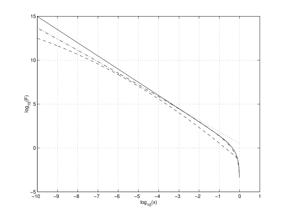
Figure 1: Comparison of the three jet fragmentation functions discussed in the text. The solid line represents the fragmentation function (5) used in this paper to calculate all ultra-high energy particle fluxes but $\nu_{\tau}$, the dash-dotted line is the from of (12), the dotted line is the approximation (13) of (12), and the dashed line is (14).

Equation (5) also applies to the primary baryonic decay products such as protons and neutrons. Assuming that 3% of the total energy of the jet goes into baryons and antibaryons and noting that most of the energy of decaying neutrons and antineutrons is transferred to daughter protons and antiprotons, the final distribution of protons and antiprotons is approximately

$$\frac{dN_{p+{\bar{p}}}}{dx}\,\simeq\,0.03\frac{15}{16}x^{-3/2}(1-x)^{2}\,.$$ (11)

Equation (5) is one approximation to the numerically computed QCD fragmentation functions, taken from Ref. HSW87 . It is derived simply by requiring that the number of decay products scales as $E^{1/2}$ and applying energy conservation and scale invariance. Further the ratio of nucleon to pions is assumed at all $x$ to equal the ratio of total nucleons to total pions per jet. Even with these reservations, we find that Eqs. (8) – (10) match the $\nu_{e}$ and $\nu_{\mu}$ spectra generated in 10 TeV $e^{+}e^{-}\rightarrow\;q\,\bar{q}\;$ events simulated by the HERWIG Monte Carlo code Herwig to within a factor of 2 in the range $10^{-4}<x<1$ MW . There are other analytical approximations of the fragmentation functions used in the literature. Another form is Hill83 ; HSW87

$$\frac{dN^{\prime}}{dx}\,\simeq\,0.08e^{2.6\sqrt{ln(1/x)}}(1-x)^{2}(x\sqrt{ln(1/x)})^{-1}\,,$$ (12)

which can be well approximated by Pijush91

$$\frac{dN^{\prime}}{dx}\,\simeq\,3.322x^{-1.324}$$ (13)

for values of $x$ between $10^{-10}<x<10^{-2}$. A third formula is based on the Modified Leading Logarithmic Approximation (MLLA) Mueller of QCD. At small $x$, the expression becomes Berez2 ; QCDbooks

$$\frac{dN^{\prime}}{dx}\,\simeq\,\frac{K}{x}exp\bigl{[}-\frac{ln^{2}x/x_{m}}{2\sigma^{2}}\bigr{]}\,,$$ (14)

where

$$2\sigma^{2}=\frac{1}{6}ln\bigl{(}\frac{m_{J}}{\Lambda}\bigr{)}^{3/2}\;,$$

$x_{m}=(\Lambda/m_{J})^{1/2}$ and $\Lambda=0.234$ GeV. Conservation of total energy in the jet

$$\int_{0}^{1}x\frac{dN^{\prime}}{dx}dx=1$$

gives the normalization constant $K$. In all approximations, extrapolations and Monte Carlo simulations of the fragmentation functions at high energies, the fraction of the jet energy carried by nucleons (or equivalently the nucleon multiplicity) lies in the range 3–10% but the precise value and dependence on $x$ and $m_{J}$ is unknown sarkar .

Fig. 1 shows a comparison of the three fragmentation functions (5), (12) and (14). The difference between these functions is small in the energy range $10^{-6}<x<10^{-0.5}$, and will be unimportant for order of magnitude considerations. Hence, in the following we will use mostly approximation (5). We stress however that no extrapolated fragmentation function should be regarded as accurate to more than an order of magnitude at highest and lowest $x$. Investment in precision in those regions of the predicted spectra is unjustified and misleading.

For the first time in cosmic string emission analysis, we also include the distribution for the tau neutrinos produced in the jet decays, which had erroneously been assumed to be negligible in all previous work. While the number of $\nu_{\tau}$ produced per $m_{J}>1$ TeV jet is less than $10^{-3}$ of the number of $\nu_{e}$ and $\nu_{\mu}$, the high energy $\nu_{\tau}$ are predominantly produced by the initial decays of the heavier quarks with shorter lifetimes and the $\nu_{e}$ and $\nu_{\mu}$ are produced by the final state cluster decays of the much lighter pions. This leads to significantly greater relative contribution from $\nu_{\tau}$ at high $x$ than previously assumed. The fragmentation distribution (5) is no longer relevant for the tau neutrino. Instead MacGibbon, Wichoski, and Webber MWW ; MW find that the fragmentation function for $\nu_{\tau}$ production in 300 GeV - 100 TeV $e^{+}e^{-}\rightarrow\;q\,\bar{q}\;$ events, as simulated by HERWIG Herwig can be parametrized as

$$\frac{dN_{\nu_{\tau}+{\bar{\nu}_{\tau}}}}{dE_{\nu_{\tau}}}\,\simeq\,\frac{1}{m_{J}}\Bigg{[}-0.36+0.15\;\biggl{(}\frac{E_{\nu_{\tau}}}{m_{J}}\biggr{)}^{-1/2}+0.27\;\biggl{(}\frac{E_{\nu_{\tau}}}{m_{J}}\biggr{)}^{1/2}-0.06\;\biggl{(}\frac{E_{\nu_{\tau}}}{m_{J}}\biggr{)}^{3/2}\Bigg{]}\;.$$ (15)

Consistent results are obtained from jet decay events simulated by PYTHIA/JETSET Lund .

The expressions for the number density of jets (4), and for the energy distribution of the jet decay products, (6), (8), (9), (10), (11) or (15), can be convolved to obtain the expected flux $F(E)$ of high energy photons, neutrinos, and cosmic rays with energy $E$ from a VHS string distribution

$$F(E)=\frac{1}{4\pi}\int_{t_{c}}^{t_{istr}}dt^{\prime}\,\frac{dn_{J}}{dt^{\prime}}\,\big{(}z(t^{\prime})+1\big{)}^{-3}\,\frac{dN}{dE^{\prime}}\,\frac{dE^{\prime}[E,z(t^{\prime})]}{dE}\;.$$ (16)

In Eq. (16), particles observed today ($t=t_{0}$) with energy $E$ were produced at a time $t^{\prime}$ with energy $E^{\prime}=E^{\prime}[E,z(t^{\prime})]$, where $z(t^{\prime})$ denotes the redshift at time $t^{\prime}$. The factor $(z(t^{\prime})+1)^{-3}$ expresses the dilution of the particle number density in an expanding Universe. The lower cutoff time $t_{c}(E)$ corresponds to the maximal redshift from which particles of present-day energy $E$ can reach us. This cutoff can be due either to interactions with the ambient extragalactic and galactic media during propagation, or to the constraint that the initial energy $E^{\prime}$ must be less than the initial jet energy $m_{J}$. The upper cutoff time $t_{istr}$ corresponds to the latest time that the emission from the VHS cosmic string network can be considered isotropic (see Section III). Thus our upper cutoff time is that from which emission will have just isotropized by today.

For protons, in order to calculate the Jacobian $\frac{dE^{\prime}[E,z(t)]}{dE}$ we apply the continuous energy loss approximation (CEL) and solve Eq. (16) numerically. The use of the CEL approximation is acceptable in this case where the distance to the sources is much larger than the attenuation length for the particle in the cosmic radiation backgrounds (see Section III).

For photons, if electromagnetic cascades are not taken yet into account (see below), we obtain (see Eq. (6) with $\alpha=1$)

$$E^{3}F_{\gamma}(E) \simeq \frac{1}{4\pi}\,\frac{5}{2}\nu\mu t_{0}^{-2}m_{J}\Bigl{(}\frac{E}{m_{J}}\Bigr{)}^{3}\Biggl{[}\frac{4}{3}((z_{max}+1)-(z_{min}+1))$$ (17)

$${}-\frac{1}{3}((z_{max}+1)^{-1/2}-(z_{min}+1)^{-1/2})\Bigl{(}\frac{E}{m_{J}}\Bigr{)}^{-3/2}$$

$${}-2((z_{max}+1)^{1/2}-(z_{min}+1)^{1/2})\Bigl{(}\frac{E}{m_{J}}\Bigr{)}^{-1/2}$$

$${}-\,\frac{1}{3}((z_{max}+1)^{3/2}-(z_{min}+1)^{3/2})\Bigl{(}\frac{E}{m_{J}}\Bigr{)}^{1/2}\Biggr{]}\,,$$

For neutrinos, if cascade off the relic neutrino background is not included, we have (see Eq. (10))

$$E^{3}F_{\nu_{e}+\bar{\nu}_{e}}(E) \simeq \frac{1}{4\pi}\,\frac{5}{2}\nu\mu t_{0}^{-2}m_{J}\Bigl{(}\frac{E}{m_{J}}\Bigr{)}^{3}\Biggl{[}{3.17}\,((z_{max}+1)-(z_{min}+1))$$ (18)

$${}-{0.24}\,((z_{max}+1)^{-1/2}-(z_{min}+1)^{-1/2})\Bigl{(}\frac{E}{m_{J}}\Bigr{)}^{-3/2}$$

$${}-{2.98}\,((z_{max}+1)^{1/2}-(z_{min}+1)^{1/2})\Bigl{(}\frac{E}{m_{J}}\Bigr{)}^{-1/2}$$

$${}-{1.38}\,((z_{max}+1)^{3/2}-(z_{min}+1)^{3/2})\Bigl{(}\frac{E}{m_{J}}\Bigr{)}^{1/2}$$

$${}-{0.01}((z_{max}+1)^{2}-(z_{min}+1)^{2})\Bigl{(}\frac{E}{m_{J}}\Bigr{)}$$

$${}+{0.14}\,((z_{max}+1)^{3}-(z_{min}+1)^{3})\Bigl{(}\frac{E}{m_{J}}\Bigr{)}^{2}$$

$${}-{0.03}\,((z_{max}+1)^{4}-(z_{min}+1)^{4})\Bigl{(}\frac{E}{m_{J}}\Bigr{)}^{3}\Biggr{]}\,,$$

for electron neutrinos and (see Eqs. (8) and (9))

$$E^{3}F_{\nu_{\mu}+\bar{\nu}_{\mu}}(E)\simeq\left\{\begin{array}[]{l}\frac{1}{4\pi}\,\frac{5}{2}\nu\mu t_{0}^{-2}m_{J}\Bigl{(}\frac{E}{m_{J}}\Bigr{)}^{3}\Biggl{[}{6.08}\,((z_{max}+1)-(z_{min}+1))\\ -\,{0.46}\,((z_{max}+1)^{-1/2}\,-\,(z_{min}+1)^{-1/2})\Bigl{(}\frac{E}{m_{J}}\Bigr{)}^{-3/2}\\ -\,{5.96}\,((z_{max}+1)^{1/2}-1)\Bigl{(}\frac{E}{m_{J}}\Bigr{)}^{-1/2}\\ -\,{2.42}\,((z_{max}+1)^{3/2}\,-\,(z_{min}+1)^{3/2})\Bigl{(}\frac{E}{m_{J}}\Bigr{)}^{1/2}\\ +\,{0.08}\,((z_{max}+1)^{3}-(z_{min}+1)^{3})\Bigl{(}\frac{E}{m_{J}}\Bigr{)}^{2}\\ -\,{0.01}\,((z_{max}+1)^{4}-(z_{min}+1)^{4})\Bigl{(}\frac{E}{m_{J}}\Bigr{)}^{3}\Biggr{]}\\ \mbox{for}\quad E\leq\frac{m_{J}}{\alpha}\;,\\ \\ \frac{1}{4\pi}\,\frac{5}{2}\nu\mu t_{0}^{-2}m_{J}\Bigl{(}\frac{E}{m_{J}}\Bigr{)}^{3}\Biggl{[}{2.96}\,((z_{max}+1)-(z_{min}+1))\\ -\,{0.24}\,((z_{max}+1)^{-1/2}-(z_{min}+1)^{-1/2})\Bigl{(}\frac{E}{m_{J}}\Bigr{)}^{-3/2}\\ -\,{2.90}\,((z_{max}+1)^{1/2}-(z_{min}+1)^{1/2})\Bigl{(}\frac{E}{m_{J}}\Bigr{)}^{-1/2}\\ -\,{1.22}\,((z_{max}+1)^{3/2}-(z_{min}+1)^{3/2})\Bigl{(}\frac{E}{m_{J}}\Bigr{)}^{1/2}\\ +\,{0.08}\,((z_{max}+1)^{3}-(z_{min}+1)^{3})\Bigl{(}\frac{E}{m_{J}}\Bigr{)}^{2}\\ -\,{0.01}\,((z_{max}+1)^{4}-(z_{min}+1)^{4})\Bigl{(}\frac{E}{m_{J}}\Bigr{)}^{3}\Biggr{]}\\ \mbox{for}\quad\frac{m_{J}}{\alpha}<E\leq m_{J}\;,\end{array}\right.$$ (19)

for muon neutrinos.

Similarly for the tau neutrinos, the flux from the string distribution neglecting cascading is (see Eq. (15))

$$E^{3}F_{\nu_{\tau}+\bar{\nu}_{\tau}}(E) \simeq \frac{1}{4\pi}\,\nu\mu t_{0}^{-2}m_{J}\Bigl{(}\frac{E}{m_{J}}\Bigr{)}^{3}\Biggl{[}{-0.36}\,((z_{max}+1)-(z_{min}+1))$$ (20)

$${}+{0.30}\,((z_{max}+1)^{1/2}-(z_{min}+1)^{1/2})\Bigl{(}\frac{E}{m_{J}}\Bigr{)}^{-1/2}$$

$${}+{0.18}\,((z_{max}+1)^{3/2}-(z_{min}+1)^{3/2})\Bigl{(}\frac{E}{m_{J}}\Bigr{)}^{1/2}$$

$${}-{0.02}\,((z_{max}+1)^{5/2}-(z_{min}+1)^{5/2})\Bigl{(}\frac{E}{m_{J}}\Bigr{)}^{3/2}\Biggr{]}\,,$$

In Eqs. (17–20), $z_{min}$ is the redshift corresponding to $t_{istr}$ and $z_{max}(E)$ is the redshift corresponding to $t_{c}$:

$$z_{max}(E)+1\,=\,min(z_{co}(E)+1,\frac{m_{J}}{E})\,,$$ (21)

where $z_{co}(E)$ denotes the redshift cutoff due to astrophysical interactions. For convenience, we have presented Eqs. (17 – 20) for the case $z_{max}(E)<z_{eq}$. In our figures, we have calculated the more general result for $z_{max}(E)>z_{eq}$ where appropriate.

The first important conclusion to draw from Eqs. (17–19) is that for energies $E$ substantially smaller than the effective initial jet energy $m_{J}$, the fragmentation term proportional to $(E/m_{J})^{-3/2}$ similarly dominates the flux of photons, electron and muon neutrinos giving

$$E^{3}F_{\gamma,\nu_{e}+{\bar{\nu}_{e}},\nu_{\mu}+{\bar{\nu}_{\mu}}}(E)\,\propto\,m_{J}^{-1/2}\,$$ (22)

In the case of the tau neutrinos the fragmentation term proportional to $(E/m_{J})^{-1/2}$ dominates the flux so that Eq. (20) gives,

$$E^{3}F_{\nu_{\tau}+{\bar{\nu}_{\tau}}}\,\propto\,m_{J}^{-3/2}\,.$$ (23)

Hence, for fixed cosmic string mass per unit length $\mu$, the spectrum of high energy photons and neutrinos increases as the jet energy $m_{J}$ decreases. This occurs because for smaller values of $m_{J}$ there are more jets emitted from the string and the fragmentation function as a function of $E$ is more compressed. These two effects overcome the $m_{J}^{3/2}$ or $m_{J}^{1/2}$ factor of the dominant term of the fragmentation function. We also note that the fluxes in the VHS scenario increase as $G\mu$ increases, or equivalently the symmetry breaking scale increases, in contrast to the general decrease seen in the standard cosmic string scenario.

To complete the calculation of the photon, neutrino and cosmic rays we need to know the values of $z_{max}(E)$. For protons and antiprotons with energy between $\sim 5\times 10^{18}$ eV and $\sim 5\times 10^{19}$ eV, the dominant interaction is $e^{+}e^{-}$ pair production off the cosmic microwave background. At higher energies, photopion production becomes the dominant energy loss mechanism. The onset of photopion production corresponds to the GZK cutoff energy GZK . Above this energy, the rate of energy loss increases dramatically, and nucleons do not reach us from cosmological distances.

Applying the results of absorp , we find, in the case of protons and antiprotons, $z_{co_{p}}(E)$ for various values of $m_{J}=\eta/2$ (where $\eta$ is the scale of the symmetry-breaking) corresponding to $G\mu=10^{-6},10^{-8},10^{-10},10^{-12},10^{-14},$ and $10^{-16}$ as shown in Fig. 2.

Figure 2: The average maximal redshift $z_{max_{p}}(E)$ from which protons and antiprotons can reach the Earth as a function of the energy at arrival. The solid lines represent from top to bottom $G\mu=10^{-6},10^{-8},10^{-10},10^{-12},10^{-14},10^{-16}$. Note the sharp decrease of the curve above $\sim 4\times 10^{19}$ eV corresponding to the GZK cutoff.

In Fig. 3 we plot the average maximum distance that a ultra-high energy proton or antiproton can travel in the CMB. After propagating $\sim 100$ Mpc the proton or antiproton energy decreases below $\sim 6\times 10^{19}$ eV irrespective of the initial jet energy. For an expanded treatment see e.g. prev .

Figure 3: Energy of a proton (antiproton) as a function of the distance of travel through the CMB, for the same 6 values of $G\mu$ (determining the initial energy) used in the previous figure.

For photons of energies greater than about $10^{11}$ eV, $z_{co_{\gamma}}(E)$ is determined by pair production off the cosmic photon background. The resulting function $z_{co_{\gamma}}(E)$ is shown in Fig. 4 (taken from Ref. JR2 ). For lower energies, pair production off nuclei determines the form of $z_{co_{\gamma}}$.

Figure 4: The maximal redshift $z_{co_{\gamma}}(E)$ from which photons can reach the Earth as a function of the energy at arrival JR2 .

For neutrinos, the dominant process is scattering off the relic $1.9^{o}$K cosmic background neutrinos. In this case, $z_{co_{\nu}}(E)$ is given by BHS92

$$z_{co_{\nu}}\,\simeq\,9\times 10^{8}\bigg{(}\frac{E}{eV}\bigg{)}^{-1/3}\,,\quad E\,\leq\,3\times 10^{14}\;eV\,$$ (24)

and

$$z_{co_{\nu}}\,\simeq\,5\times 10^{8}\bigg{(}\frac{E}{eV}\bigg{)}^{-2/7}\,,\quad E\,\geq\,3\times 10^{14}\;eV\,.$$ (25)

The decay of lepton pairs produced in the neutrino scattering process further enhances the spectrum of all neutrino species and allows neutrino emission, corresponding to present day energies $E\leq 10^{21}$ eV, to be detected from significantly higher redshifts than those given in (24) and (25) Yoshida . The cascade enhancement due to decay is only relevant at high redshift where the neutrino mean free path is sufficiently small. In the case of electron and muon neutrinos, we will neglect the cascade enhancement of $z_{co_{\nu}}$ because the dominant term in the neutrino flux from VHS strings, (18) and (19), is proportional to $(1-(z_{max_{\nu}}+1)^{-1/2})$ and the modifications to the $\nu_{e}$, $\nu_{\mu}$, and $\nu_{\tau}$ spectra expected at Earth are negligible above $E\sim 10^{-3}m_{X}$ Yoshida . The cascade enhancement at low energies increases as $m_{X}$ increases due to the greater energy in the initial jets.

III Comparison with Observations

As we mentioned above, the diffuse fluxes of particles in the VHS scenario are produced directly by the decay of X-particles. The X-particles decay immediately after they are radiated from the long string segments. The result is that the particle fluxes are produced along the strings. The number of long strings per Hubble volume $\nu$ we noted in Section I is approximately 13. As the Universe expands the comoving inter-string distance grows as

$$D_{ints}\propto\frac{2}{\sqrt{\nu}}(1+z)^{-1/2}H_{o}^{-1}\;.$$ (26)

Fig. 5 depicts the evolution of the average distance between long string segments. The distance between the observer and a long string segment, $D_{ls}$ is estimated to be

$$D_{ls}\sim\frac{D_{ints}}{\sqrt[3]{2}}\;.$$

If the distance today between the observer and the long string segment is larger than the maximum average propagation distance for particles arriving with an energy $E$ then the fluxes at Earth are exponentially suppressed Berez . Based on Eq. (26) we see that presently the average distance to a long string segment is

$$D_{0,ls}\simeq 2000\;\mbox{Mpc},$$ (27)

which corresponds to a redshift $z_{ls}\simeq 0.58$.

The present average redshift to a long string segment $z_{ls}$ can be taken as a rough estimate of $z_{min}$, i.e., of the redshift corresponding to the latest time ($t_{istr}$) that the emission from the VHS string network can be considered isotropic. This sets an upper limit of the integral (16) and consequently in Eqs. (17–20) we have

$$z_{min}=z_{ls}\simeq 0.58\;.$$ (28)

Hence only the particle fluxes emitted from the VHS network before $t_{istr}$ ($z>z_{min}$) are relevant for the diffuse flux.

A segment of long string could be substantially closer than $D_{0,ls}$, the expected average distance to the nearest string. In this case, a flux of cosmic rays protons (antiprotons) and photons above the GZK cutoff might be observed. However, these fluxes would be highly anisotropic in contradiction to the present observations of UHE events above the GZK cutoff agasanew .

Figure 5: Average distance between long string segments as a function of the redshift.

III.1 Protons

In what follows, we discuss the proton flux. Because the fragmentation functions and relevant interactions with the cosmic backgrounds are to first order charge symmetric, the expected antiproton flux from the VHS strings is the same as the proton flux.

The average maximum distance at the present time to the source of a proton arriving with energy $\sim 4\times 10^{19}$ eV (the onset of the GZK cutoff) is $\lesssim 160$ Mpc (see Fig. 3). This is equivalent to the source being at a redshift $z\lesssim 0.036$, much smaller than the distance from which the flux can be considered isotropic ($\simeq 2000$ Mpc). It implies that no isotropic flux of protons from VHS strings is expected at Earth above the GZK cutoff. On the other hand, a diffuse proton flux from the strings should reach the Earth at arrival energies $E\lesssim 6\times 10^{18}$ eV, well below the UHE event energies. Although no isotropic flux of protons at UHE energies is expected at Earth, the UHE protons emitted at high redshifts will have interacted with the universal radio background (URB), CMB, and the infra-red/optical (IR/O) backgrounds to produce secondary fluxes of $\gamma$-rays, electrons, and neutrinos. These secondary fluxes could in principle be used to constrain the VHS model. However, in the context of the TD scenarios including the VHS scenario, these nucleon-induced secondary fluxes are negligible compared to the corresponding fluxes directly produced by the decay of the X-particles. This is because in the X-particle decay, far more direct $\gamma$-rays and neutrinos are produced than nucleons.

III.2 Photons and Charged Leptons

The maximum redshift at which a photon arriving today with an energy $E$ could have been emitted is given in Fig. 4. If we compare this redshift to the present average distance to a long string ($z_{ls}\simeq 0.58$) we would deduce that the isotropic UHE $\gamma$-ray flux should also be exponentially suppressed. In the case of $\gamma$-rays, this is not the full story. Fig. 4 describes the interaction length of the photons, i.e., the distance traveled by a UHE photon before it is absorbed in the cosmic backgrounds. The UHE photons initiate electromagnetic cascades as they travel in the cosmic backgrounds. An important consequence is that the effective penetration length of the cascade is considerably larger than the interaction length Bonom . In the VHS scenario, both the interaction length and the effective penetration length are much smaller than the distance to the nearest expected string (cf. Eq. (26)). The result is that the $E\gtrsim 10^{11}$ eV $\gamma$-ray are essentially subtracted from the arriving flux: The flux above $E\sim 10^{20}$ eV is depleted due to interactions with the URB; the flux in the range $10^{14}\lesssim E\lesssim 10^{20}$ eV is depleted by the CMB; and the flux in the range $10^{11}\lesssim E\lesssim 10^{14}$ eV is depleted by the IR/O backgrounds. The energy lost by the photons emitted with energies above $\sim 10^{11}$ eV at high redshifts is recycled into energies below $E\gtrsim 10^{11}$ eV. Analytic calculations ancascades have shown that the electromagnetic cascade spectrum has a generic shape below $\gtrsim 10^{13}$ eV, i.e., the secondary cascade radiation spectrum is insensitive to the injection spectrum. This implies that, even in the absence of the detection of direct UHE photons, the $\gamma$-ray flux below $E\gtrsim 10^{11}$ eV can be used to constrain the VHS scenario. The charged leptons created in the X-particle decay also initiate electromagnetic cascades on the cosmic backgrounds. As in the case of the UHE photons, the energy of the UHE charged leptons is recycled and enhances the photon flux below $\gtrsim 10^{11}$ eV.

The constraints on the electromagnetic emission in TD models with a spectral index $p=1$, which is applicable to the VHS scenario, stem from the limits on the present diffuse $\gamma$-ray background between $3\times 10^{6}$ eV and $10^{11}$ eV egret . These require that SJSB ; ProtSta ; SLBY ; CA

$$Q_{EM}^{0}\lesssim 3\times 10^{-23}\;\mbox{eV}\;\mbox{cm}^{-3}\;\mbox{sec}^{-1}\;,$$ (29)

for $h=0.65$ where $Q_{EM}^{0}$ is the present rate of total energy injection into the electromagnetic channels.

In the VHS scenario, we have from Eq. (4) that the present rate of total energy injection into the electromagnetic channel (photon and charged lepton emission) is

$$Q_{EM-VHS}^{0}\sim 2.3\times 10^{-12}\;\left[\frac{1}{2}\right]\;\left[\frac{\nu}{13}\right]\left[G\mu\right]\left[\frac{h}{0.65}\right]^{3}\;\mbox{eV}\;\mbox{cm}^{-3}\;\mbox{sec}^{-1}\;.$$ (30)

Comparing to the $Q_{EM}^{0}$ limit in (29), we obtain a constraint on the energy density of a string in the VHS scenario of

$$G\mu\lesssim 3\times 10^{-11}\;.$$ (31)

Here we have assumed an extragalactic magnetic field of $B_{exgal}\lesssim 10^{-11}$ G. Stronger values of the extragalactic magnetic field generate greater initial synchrotron losses at ultra-high energies, decreasing the UHE spectra, enhancing the cascade reprocessing into low energies, and thus lowering the upper limits on $Q_{EM}^{0}$ and $G\mu$. Because of the large distances to the sources, we have also neglected the uncertainties in the cosmic background URB and IR/O intensities CA .

III.3 Neutrinos

The predicted flux of high energy neutrinos in the VHS scenario can be obtained from Eqs.(18 - 20) using (21), (24), and (25) to determine $z_{max_{\nu}}$. The resulting $\nu_{e}$ and $\nu_{\mu}$ fluxes are shown in Fig. 6 and the $\nu_{\tau}$ flux in Fig. 7, for the case when $m_{J}=\eta/2$ where $\eta$ is the scale of symmetry breaking.

The cascading of the tau neutrinos off the relic neutrino backgrounds will have little effect on the tau neutrino spectrum shown in Fig. 7. However, a secondary $\nu_{\tau}$ component peaking at lower energies will be created in collisions of the string-produced $\nu_{e}$ and $\nu_{\mu}$ with the relic neutrino backgrounds. This $\nu_{e}$ and $\nu_{\mu}$ cascading should increase the net $\nu_{\tau}$ flux below $x\sim 10^{-3}$. The $\nu_{\tau}$ signal expected at Earth from VHS strings will be the sum of these two components, as shown in Fig. 8 for $G\mu\sim 10^{-8}$ MWW ; MW . In Fig. 8 we have plotted the cascade component calculated in Ref. Yoshida for a $p=1$ TD scenario. This is only an estimate because the distance distribution of strings varies from model to model. We will address full modeling of the $\nu_{\tau}$ flux including cascades in a later paper. Note however that it is the high $x$ region, where the cascades have little effect, which is the most observationally interesting.

Our new result is that the $\nu_{e}$, $\nu_{\mu}$ and $\nu_{\tau}$ fluxes are of similar magnitude as $E\rightarrow m_{J}$, unlike all previous string emission calculations which predicted a negligible $\nu_{\tau}$ component at high $x$. In other string emission or X-decay scenarios, the $\nu_{e}$, $\nu_{\mu}$ and $\nu_{\tau}$ flux should also be of comparable magnitude as $x\rightarrow 1$. Because of the uncertainty in extrapolating to high emission energies, the precise ratio of the neutrino fluxes at high $x$ is not known (also, as plotted in Fig. 8, the extrapolation for $\nu_{\tau}$ is derived from HERWIG Monte Carlo simulations while the $\nu_{e}$ and $\nu_{\mu}$ functions are derived from the less rigorous approximation Eq. (5).) The actual ratio will be determined by the first step in the X-decay chain which is unknown and may be influenced by, for example, leptonic and SUSY decay channels (see Section IV).

Figure 6: Electron and muon neutrino fluxes in the VHS cosmic string scenario (for $m_{J}=\eta/2$) for various values of $G\mu$ (lines from top to bottom, $G\mu=10^{-6}$, $10^{-8},10^{-10},10^{-12},10^{-14},10^{-16}$). The solid lines represent the $\nu_{\mu}$ flux and the dashed lines represent the $\nu_{e}$ flux. Points with arrows represent upper limits on the diffuse neutrino flux from the EAS-TOP eastop , the Fréjus frejus and the Fly’s Eye eye experiments. The upper limits stemming from the projected sensitivities for both the Pierre Auger project auger and the OWL/Airwatch project owlairwatch are also plotted.

The most recent observational limits come from the EAS-TOP eastop , the Fréjus frejus , and the Fly’s Eye eye experiments. These experiments give upper limits on the cosmic ray neutrino flux in the energy range between $10^{13}$ eV and $10^{20}$ eV. In Figs. 6 and 7 we have plotted the observational limits using the updated $\sigma_{CC}(\nu N)$ cross-section Quigg . By inspection, we see that the most stringent constraint comes from the highest energy $\nu_{\mu}$ flux in Fig. 6 which gives an upper bound on $G\mu$ of

$$G\mu\,\lesssim\,10^{-10}\,.$$ (32)

This bound is derived at high $x$ so it should be little affected by the cascades which are neglected in Fig. 6.

Figure 7: Tau Neutrino flux in the VHS cosmic string scenario (for $m_{J}=\eta/2$) for various values of $G\mu$ (lines from top to bottom, $G\mu=10^{-6}$, $10^{-8},10^{-10},10^{-12},10^{-14},10^{-16}$). For each value of $G\mu$, the range of energies where the $\nu_{\tau}$ from decays dominates the total $\nu_{\tau}$ flux is depicted by the solid section of the line. Points with arrows represent upper limits on the diffuse neutrino flux as in the previous figure.

We have also plotted on Figs. 6 and 7 the upper limits stemming from the planned sensitivities of the Pierre Auger project as estimated in Ref. auger , and the OWL/Airwatch project as estimated in Ref. owlairwatch . It is assumed that both experiments will collect data over a period of a few years. Their sensitivities span the energy range between $10^{19}$ eV and $10^{22}$ eV and would allow more stringent upper limits on $G\mu$ up to

$$G\mu\,\lesssim\,10^{-12}\,,$$ (33)

in the case of null detection by the Pierre Auger project; and

$$G\mu\,\lesssim\,10^{-14}\,,$$ (34)

in the OWL/Airwatch case. Unlike the present constraint (32), the Auger and OWL/Airwatch projects will constrain the $\nu_{\mu}$ flux in Fig. 6 at energies $E\sim 10^{19}$ eV (i.e. the lower end of the energy range of these experiments). The $\nu_{\tau}$ flux is below the present observational upper limits. The $\nu_{\tau}$ sensitivities of future experiments are expected to constrain $G\mu$, but these constraints are expected to be an order of magnitude weaker than those from the $\nu_{e}$ and $\nu_{\mu}$ fluxes. The slope of the $\nu_{\tau}$ spectrum is steeper than the slope of the observational upper limits for both present and future data (cf. Fig. 7). On the other hand, the $\nu_{\tau}$ component of a TD signature maybe easier to distinguish from other sources than the $\nu_{e}$ and $\nu_{\mu}$ components.

As is obvious from (22), (23) and Fig. 9 the predicted flux of cosmic ray neutrinos increases as $m_{J}$ decreases. Thus, the VHS scenario with GUT-scale strings cannot be made compatible with observational constraints by lowering the energy scale $m_{J}$ of the initial jets (which likely happens if new physics evolves between the electroweak symmetry breaking scale and the GUT scale). Raising $m_{J}$ above $\eta$ would alleviate the conflict, but this appears quite unnatural.

Figure 8: Neutrino flux in the VHS cosmic string scenario for various values of $G\mu=10^{-8}$ The solid line represent the $\nu_{\mu}$ flux, the dashed lines represent the $\nu_{e}$ flux, and the dotted line the $\nu_{\tau}$ flux. The dash-dotted line represents the $\nu_{\tau}$ from the cascade of $\nu_{e}$ and $\nu_{\mu}$ due to the interactions with the relic neutrino background. Points with arrows represent upper limits on the diffuse neutrino flux as in the previous figures.

The initial decay channels and branching ratios for the X-particle are unknown. The application of the extrapolated QCD-derived fragmentation functions to X-decay assumes implicitly that the branching ratios for $X\rightarrow q_{i}+\bar{q_{i}}$ are the same as those for $e^{+}e^{-}\rightarrow q_{i}+\bar{q_{i}}$. This may not be so for even hadronic decays at very high energies. The initial decay channel $X\rightarrow q+l_{X}$, where $l_{X}$ is a charged lepton, should produce spectra which are decreased by no more than a factor of 2, compared with the $X\rightarrow q+\bar{q}$ spectra (assuming equi-partition of the X-particle energy between the initial $q$ and $l_{X}$), with the exception of an $\nu_{\tau}$ spectrum enhancement as $E\rightarrow m_{X}/2$ due to decay of the initial $\tau$ MWW ; MW . The initial charged lepton $l_{X}$ would also generate EM cascades which are effectively attenuated at high energies in the VHS scenario, as we remarked in Section II for the other EM decay products, but which would contribute to the spectra at low energies. This should increase the total energy going into the EM cascade channel by less than $\sim 50\%$ (see Eq. (30)). Pure leptonic decay channels $X\rightarrow l_{X}+l^{\prime}_{X}$, $X\rightarrow l_{X}+\nu_{X}$ or $X\rightarrow\nu_{X}+\nu^{\prime}_{X}$ would produce substantially suppressed spectra, because of the low multiplicity per decay compared with hadronic jets, except for a possible neutrino spectra increase as $E\rightarrow m_{X}/2$ due to the initial step in the decay chain. In the case of purely leptonic decays, the nucleon and $\gamma$-ray spectra would be wholly created by the collisions of the emitted leptons with the cosmic ambient media. It has been shown that in TD models generally, pure leptonic decays can only be made interesting if the cosmic relic neutrinos are massive, non-relativistic and locally clustered thus enhancing the relative cascade-generated component (Ref. SLBY ). However, it is highly unlikely that the X-particles (being high energy gauge and scalar particles) would decay purely into leptons in the initial step. Because of the much higher multiplicity of hadronic jets, any scenario containing reasonable initial branching ratios for the X-particle (say, to within a factor of 2–3: $30\%$ pure hadronic, $30\%$ pure leptonic and $30\%$ hadronic and leptonic) would produce spectra dominated by the particles produced via the hadronic decay channels. Hence, even in the case of locally clustered relic neutrinos, the component produced in pure leptonic decays would be essentially dominated by the hadronic decays, with the possible exception of a UHE neutrino feature as $E\rightarrow m_{X}/2$.

Figure 9: Electron and muon neutrino fluxes in the VHS cosmic string scenario for $G\mu=10^{-6}$ and $m_{J}\sim 10^{25},10^{23},10^{21},10^{19},10^{17}$ eV (lines from bottom to top). The solid lines represent the $\nu_{\mu}$ flux and the dashed lines represent the $\nu_{e}$ flux. Points with arrows represent upper limits on the diffuse neutrino flux as in the previous figures.

IV Extensions to the Model

In the analysis so far, we have assumed $m_{\nu}=0$. If neutrinos do possess a small mass, as present neutrino oscillation experiments hint, the predicted spectra from VHS strings are modified in two ways. Firstly, the interaction of the string-produced neutrinos with the $1.9^{o}$K relic background neutrinos is strongly enhanced at the resonance for $Z^{0}$ production Weiler , $E_{res}=m_{Z}^{2}/2$ $m_{\nu}\sim 4\times 10^{21}/(m_{\nu}/\mbox{eV})$ eV. (If neutrinos are massless, the $Z^{0}$ resonance occurs at $E_{res}\sim 3\times 10^{24}$ eV Yoshida .) The present upper limits from particle physics experiments on the neutrino masses are $m_{\nu_{e}}\lesssim 3$ eV, $m_{\nu_{\mu}}\lesssim 0.19$ MeV, and $m_{\nu_{\tau}}\lesssim 18.2$ MeV RPP . The cosmological requirement that $\Omega_{m}\leq 1$ places a stricter upper limit on the sum of the masses of the three neutrino species of $\lesssim 92h^{2}$ eV Bludman . Taken together these limits imply that at least one $Z^{0}$ resonance must occur for neutrinos today at some energy in the range $10^{20}$ eV $\lesssim E_{res}\lesssim 3\times 10^{24}$ eV. The exact value(s) of $E_{res}$ will depend on whether or not the neutrinos have mass, and the value(s) of the neutrino mass(es) if non-zero. If the neutrino masses are non-degenerate, the $Z^{0}$ resonance will occur at two or three distinct $E_{res}$ in this range. In the case that $E_{res}<m_{X}$, the $Z^{0}$ resonance in the VHS scenario will produce a slight decrease in the predicted neutrino fluxes around $E_{res}$ and in the energy decade below $E_{res}$, and an accompanying slight enhancement on all spectra below $\sim 10^{-2}E_{res}$ due to secondary $Z^{0}$ decay products. The amplitudes of all spectra should be modified by less than a factor of 2. (See for example Ref. Yoshida for the case of degenerate $m_{\nu}=1$ eV neutrinos in other cosmic string models.) If the relic neutrinos are non-relativistic and clustered locally on a scale less than the attenuation length for photons and nucleons, the effect on the photon, proton and antiproton spectra may be enhanced YSL .

Secondly, a non-zero neutrino mass may lead to oscillations between neutrino species as the flux propagates to Earth. In this case, the total number of neutrinos is preserved but the ratio of the flux in each species may depend on the neutrino energy, the distance traveled and neutrino masses. Recent observations by the SuperKamiokande, Kamiokande, MACRO and Soudan experiments of $\nu_{e}$ and $\nu_{\mu}$ neutrinos produced by cosmic rays colliding with the Earth’s atmosphere strongly suggest that neutrino oscillations (at least between the $\nu_{\mu}$ and $\nu_{\tau}$ flavors) occur. [For a review of the current status of neutrino oscillation experiments and measurement implications see Akhm and references therein]. The evidence for zenith-angle dependence in the SuperKamiokande data further strengthens this interpretation. Similarly, the long-standing observed deficit of solar neutrino flux may be resolved by $\nu_{e}$ oscillation into $\nu_{\mu}$ or $\nu_{\tau}$ although the solar neutrino experiments are not yet sufficiently consistent to favor a particular solution. The third set of evidence for neutrino oscillations comes from the LSND Collaboration accelerator experiment which has seen evidence for $\nu_{\mu}$ into $\nu_{e}$ oscillations. When combined with the atmospheric and solar data, this would require the existence of a fourth ”sterile” neutrino species. The LSND measurements have yet to be independently confirmed. A number of new experiments are presently being commissioned with the objective of resolving these matters. The K2K, NuM-MINOS and CNGS experiments are expected to provide the definitive answer and exploration of the relevant parameter space. In these experiments, neutrino beams will be sent from accelerators to detectors over baselines of hundreds of kilometers. K2K is already taking data and the NuM-MINOS and CNGS will be operational in 2002 and 2005, respectively.

Ignoring for now cosmological evolution, the probability of a relativistic neutrino undergoing vacuum flavor transition when propagating a distance $L$ is

$$P_{\nu_{\mu}\rightarrow\nu_{\tau}}=sin^{2}(2\,\theta_{0})\,sin^{2}\Big{(}\frac{\Delta m_{atm}^{2}\,L}{4\hbar cE}\Big{)} = sin^{2}(2\,\theta_{0})\,sin^{2}\Biggl{[}3.9\times 10^{25}$$ (35)

$${}\times\Big{(}\frac{\Delta m_{atm}^{2}}{10^{-3}\ \mbox{eV}^{2}}\Big{)}\Big{(}\frac{L}{\mbox{Mpc}}\Big{)}\Big{(}\frac{E}{\mbox{eV}}\Big{)}^{-1}\Biggr{]}$$

in the 3-flavor solution. The atmospheric data to date are best fit by an amplitude of $sin^{2}(\theta_{0})=0.82-1.0$ and a mass difference of $\Delta m_{atm}^{2}=(2-6)\times 10^{-3}\mbox{eV}^{2}$ Akhm . For models with distant cosmological sources (e.g. TDs and AGNs) and a neutrino ratio at emission of $F_{\nu_{e}}:F_{\nu_{\mu}}:F_{\nu_{\tau}}\simeq 1:2:0$ (in our case this occurs at $E<<m_{J}$), the ratio of the spectra reaching the Earth will be $F_{\nu_{e}}:F_{\nu_{\mu}}:F_{\nu_{\tau}}=1:1:1$ in the 3-flavor model; similarly, in the 4-flavor model consistent with the LSND data, an initial emission ratio of $F_{\nu_{e}}:F_{\nu_{\mu}}:F_{\nu_{\tau}}:F_{\nu_{s}}\simeq 1:2:0:0$ will become $F_{\nu_{e}}:F_{\nu_{\mu}}:F_{\nu_{\tau}}:F_{\nu_{s}}=1:1:1:0$ at Earth AHu . Since we showed earlier that the current average distance to the nearest long string is 2000 Mpc, even the highest energy neutrinos emitted in the present era will have undergone transition before reaching Earth. In this case, at $E<<m_{J}$, both the $\nu_{\mu}$ and $\nu_{\tau}$ flux reaching Earth should approximately equal half the $\nu_{\mu}$ flux expected without oscillations. In the case of the flux emitted in previous epochs, this will only be so provided the wavelength of the oscillation is much less than the mean free path of the $\nu_{\mu}$ and $\nu_{\tau}$ in the Universe. If the oscillation wavelength is greater than the mean free path then the cascade structure will be determined by the original neutrino flavors at emission. The mean free path decreases sharply as $z$ increases Yoshida . For example, a $10^{23}$ eV neutrino at $z\sim 10^{2}$ has a mean free path of $\sim 100$ kpc Yoshida . Since these too are the redshifts and energies at which cascading becomes relevant, cascade development should be predominantly determined by the neutrino flavors at emission. In the VHS scenario, however, the neutrino cascades have little influence on our regions of interest. Hence the predicted observable $\nu_{\mu}$ and $\nu_{\tau}$ VHS fluxes in the case with neutrino oscillations should be approximately half the unoscillated $\nu_{\mu}$ flux at $E<<m_{J}$. As $E\rightarrow m_{J}/2$, i.e. in the region where the initial $\nu_{e}$, $\nu_{\mu}$, and $\nu_{\tau}$ VHS fluxes are of comparable magnitude, the ratio should also approach $F_{\nu_{e}}:F_{\nu_{\mu}}:F_{\nu_{\tau}}\simeq 1:1:1$ in the case with neutrino oscillations. The precise value of the modulated neutrino flux $F_{\nu_{i}}$ as $E\rightarrow m_{J}/2$ will depend on the initial absolute and relative string-produced fluxes which we regard as uncertain by more than a factor of 2.

Additionally, one possible solution to the solar neutrino deficit problem is vacuum $\nu_{e}\rightarrow\nu_{\mu}$ or $\nu_{\tau}$ oscillations with $\Delta m_{\odot}^{2}\sim 10^{-10}\mbox{eV}^{2}$ and $sin^{2}2\theta_{\odot}\sim 0.6-1.0$. In this case, the phase of the transition probability, $\phi_{\odot}=\Delta m_{\odot}^{2}L/(2\hbar cE)$, is $\lesssim 1$ for $E\gtrsim 10^{21}$ eV neutrinos emitted today from a long string at 2000 Mpc. Thus the $\nu_{e}$ spectra at Earth would be determined by $\nu_{e}\rightarrow\nu_{\mu}$ or $\nu_{\tau}$ oscillation below $E\sim 10^{21}$ eV and exhibit negligible $\nu_{e}$ oscillation above $E\sim 10^{21}$ eV. If this particular solar deficit solution is combined with the solution implied by the atmospheric data $\Delta m_{atm}^{2}\sim 10^{-3}\;\mbox{eV}^{2}$, an initial ratio at emission of $F_{\nu_{e}}:F_{\nu_{\mu}}:F_{\nu_{\tau}}\simeq 1:2:0$ or $F_{\nu_{e}}:F_{\nu_{\mu}}:F_{\nu_{\tau}}\simeq 1:1:1$ would be modulated to $F_{\nu_{e}}:F_{\nu_{\mu}}:F_{\nu_{\tau}}\simeq 1:1:1$ reaching Earth because the wavelength for $\nu_{\mu}\rightarrow\nu_{\tau}$ oscillation is much smaller than that of the oscillation solution associated with the atmospheric solar data. A detailed analysis of the detector signatures for various oscillation scenarios is presented in Refs. DRS1 and DRS2 .

Other extensions to the Standard Model could influence the predicted spectra. The existence of a supersymmetric (SUSY) sector would contribute extra decay channels in the fragmentation of the X-particle and jets. (See BK and references therein for possible approaches to modeling SUSY channels for application to UHE decays). The net effect would be a skewing of the primary flux spectra to lower energies and a decrease in the energy reprocessed in high energy cascades. For example, in the p=1 TD model studied in Ref. SLBY with $m_{X}=10^{16}$ GeV, including a SUSY sector decreases the spectra of all species expected at Earth by an order of magnitude at $E\gtrsim 10^{-2}m_{X}$, shifts the UHE peaks in the spectra to lower energies by at least an order of magnitude and increases the amplitude of the $\nu_{e}$, $\nu_{\mu}$, $p$ and $\bar{p}$ spectra by about an order of magnitude at energies below the peaks. The predicted $E\lesssim 10^{15}$ eV photon spectrum, predominantly generated by EM cascades, though is unchanged because the same fraction of initial X-particle energy is reprocessed into low energies in the EM cascades with or without a SUSY sector in that model. In the case of the VHS scenario, these remarks must be convolved with the suppression of the UHE $\gamma$-ray and nucleon spectra due to the nearest string being farther than the relevant UHE attenuation lengths.

To date there is no experimental evidence for a SUSY sector and no unique theoretical predictions for the architecture of the SUSY sector and superparticle properties such as mass. Other extensions to the Standard Model, for example Technicolor or Leptoquarks, which also increase the number of degrees of particle freedom would be expected to similarly skew the spectra to lower energies. As well, extensions to the Standard Model may modify the high-energy cross-sections governing the interactions of the emission with the cosmic ambient media.

V Conclusions

We have computed the ultra-high energy $\gamma-$ray, neutrino and cosmic ray fluxes in the VHS cosmic string scenario, in which the long string network loses its energy directly by particle emission. This is in contrast to the standard cosmic string model with a scale-invariant distribution of string loops which lose energy predominantly by gravitational radiation. The predicted particle fluxes are much larger in the VHS scenario.

The predictions for the particle fluxes depend on extrapolating the QCD fragmentation function to energies much higher than current accelerator energies. New physics between the QCD scale and the scale $\eta=\sqrt{\mu}$ at which the defects are formed could significantly affect the final particle distributions. We parametrize this uncertainty by introducing a scale $m_{J}$ as the energy scale to which the QCD fragmentation functions can be extrapolated and regard $m_{J}$ as the initial jet energy. The smaller the value of $m_{J}$, the larger the number of jets which are generated by the initial emission from the cosmic string. We calculate the resulting particle fluxes as a function of both $m_{J}$ and $\mu$. A new aspect of our work is the computation of the significant tau neutrino fluxes directly produced by decay in the particle jets.

Our calculations show that the predicted flux $F(E)$ of $\gamma-$rays, electron and muon neutrinos and cosmic rays scales as $E^{3}F(E)\sim E^{3/2}$, as in other defect models, whereas the present observations show a much weaker increase with $E$. Hence, the most stringent constraints on topological defect models come from the highest energies for which data exist.

Setting $m_{J}=\sqrt{\mu}/2$, the VHS strings with $G\mu\gtrsim 10^{-10}$ produce electron and muon neutrinos in excess of the UHE observations. Thus, assuming that the strings evolve as in the VHS scenario, models with $G\mu\gtrsim 10^{-10}$ or, equivalently a symmetry breaking scale of $\eta\gtrsim 10^{23}$ eV, are ruled out by the UHE data. (This result is in accordance with the limit on $G\mu$ in Ref. Pijush98b ). At a given particle energy, the predicted fluxes reaching the Earth scale as $m_{J}^{-1/2}$ and increase with $G\mu$. Lowering $m_{J}$ increases the disagreement between predictions and observations, although the upper cutoff on the predicted spectra diminishes.

A consistent but slightly stronger constraint on the VHS string scenario comes from the cascading of the electromagnetic emission off the cosmic radiation backgrounds and the potential conflict with the observed diffuse $3\times 10^{9}$ eV $\lesssim E\lesssim$ $10^{11}$ eV gamma ray background as probed by EGRET. This requires $G\mu\lesssim 10^{-11}$.

We conclude that, generically, GUT-scale strings are ruled out in the VHS scenario. However, VHS models with lighter $G\mu$, corresponding to lower symmetry-breaking scales, may be contributing interestingly to the observed UHE events. We reiterate that the VHS scenario is not universally accepted as giving the correct dynamics of cosmic strings.

Finally, we note that the uncertainties inherent in the calculation of the expected fluxes in any TD model mean that the absolute and relative flux in each particle species should not be regarded as accurate to more than an order of magnitude in any model. The list of uncertainties includes: the mass and other properties of the X-particle(s); the form of the potential of the scalar field at string formation; the branching ratios and decay channels of the X-particle(s); the validity of the extrapolated fragmentation functions; the possibility of new particles (e.g. a SUSY sector) and other extensions to the Standard Model which may influence particle production, decay and propagation; the strength of the extragalactic magnetic field; the intensity of the cosmic IR background; and the Hubble constant. Taken together, these factors have the capability to increase or decrease the absolute and relative fluxes expected at Earth.

Neutrino Flux from Muon Decay

In the main text we computed the flux of particles resulting from two-body decay of charged pions in a jet. The muons which are produced in this decay are unstable and in turn decay via a three body decay process producing electrons, muon neutrinos and anti-electron neutrinos. In this Appendix we compute the full spectra neutrinos from the $\pi^{\pm}\rightarrow\mu^{\pm}\rightarrow\nu$ decay chain.

Because of the finite muon rest mass, the muon and muon neutrinos created in the first stage of charged pion decay cannot carry an arbitrary fraction of the pion energy. In the limit $E_{\pi}\gg m_{\mu}$, the energies of the decay products lie between

$$E\,\in\,\bigl{[}0,\alpha^{-1}E_{\pi}\bigr{]}$$ (36)

for muon neutrinos and

$$E\,\in\,\bigl{[}rE_{\pi},E_{\pi}\bigr{]}$$ (37)

for muons Stecker ; Halzen . Here, $r=\bigl{(}\frac{m_{\mu}}{m_{\pi}}\bigr{)}^{2}=1-\alpha^{-1}$ where $\alpha$ is given by (7). The muon distribution is then

$$\frac{d\mu}{dE_{\mu}}=\alpha E_{\pi}^{-1}\;.$$ (38)

In order to obtain the $\nu_{\mu}$-flux, we integrate (5) over the range (36), resulting in (6). To obtain the flux of muon decay products, we follow the method of Ref. Gaisser . In the laboratory frame the distribution of leptons with energy $E=yE_{\mu}$ produced by the decay of a muon of energy $E_{\mu}$ is given by [Gaisser Gaisser p. 92]

$$\frac{dn}{dy}=g_{0}(y)-P_{\mu}g_{1}(y)$$ (39)

in the limit $E_{\mu}\gg m_{\mu},m_{e}$, where

$$g_{0}(y)=\frac{5}{3}-3y^{2}+\frac{4}{3}y^{3}$$

$$g_{1}(y)=\frac{1}{3}-3y^{2}+\frac{8}{3}y^{3}$$

for $\nu_{\mu}$ and

$$g_{0}(y)=2-6y^{2}+4y^{3}$$

$$g_{1}(y)=-2+12y-18y^{2}+8y^{3}$$

for $\nu_{e}$. In (39), $P_{\mu}$ is the projection of the muon spin in the muon rest frame along the direction of the muon velocity in the laboratory frame

$$P_{\mu}=\frac{2E_{\pi}r}{E_{\mu}(1-r)}-\frac{1+r}{1-r}\;.$$

Convolving the distribution (39) with the distribution of muons from pion decay (38) and integrating over muon and pion energies, the neutrino spectrum in the laboratory frame is

$$\frac{dN}{dE_{\nu}}=\int_{E_{\nu}}^{m_{J}}dE_{\pi}\int_{E_{min}}^{E_{\pi}}\frac{dE_{\mu}}{E_{\mu}}\frac{dN}{E_{\pi}}\frac{d\mu}{E_{\mu}}\frac{d\mu}{y}\;,$$ (40)

$$E_{min}=min[rE_{\pi},E_{\nu}]\;.$$

For simplicity we will first evaluate (40) for an initial pion distribution of the form

$$\frac{dN}{dE_{\pi}}=KE_{\pi}^{-a}\;,\hskip 56.9055pta>0\;.$$

Changing the order of integration,

$$\int_{E_{\nu}}^{m_{J}}dE_{\pi}\int_{E_{min}}^{E_{\pi}}dE_{\mu}\rightarrow\int_{E_{\nu}}^{m_{J}}dE_{\mu}\int_{E_{\mu}}^{E_{\mu}/r}dE_{\pi}\;,$$

the result is

$$\frac{dN}{dE_{\nu}}=KE_{\nu}^{-a}\frac{1-r^{a}}{a(1-r)}\biggl{[}f_{0}+\frac{f_{1}}{1-r}\Bigl{[}1+r-\frac{2ar}{a-1}\Bigl{(}\frac{1-r^{a-1}}{1-r^{a}}\Bigr{)}\Bigr{]}\biggr{]}$$ (41)

where

$$f_{0}=\frac{2(a+5)}{a(a+2)(a+3)}-\frac{5}{3a}\bigg{(}\frac{E_{\nu}}{m_{J}}\bigg{)}^{a}+\frac{3}{(a+2)}\bigg{(}\frac{E_{\nu}}{m_{J}}\bigg{)}^{a+2}-\frac{4}{3(a+3)}\bigg{(}\frac{E_{\nu}}{m_{J}}\bigg{)}^{a+3}$$

$$f_{1}=\frac{2(1-a)}{a(a+2)(a+3)}-\frac{1}{3a}\bigg{(}\frac{E_{\nu}}{m_{J}}\bigg{)}^{a}+\frac{3}{(a+2)}\bigg{(}\frac{E_{\nu}}{m_{J}}\bigg{)}^{a+2}-\frac{8}{3(a+3)}\bigg{(}\frac{E_{\nu}}{m_{J}}\bigg{)}^{a+3}$$

for $\nu_{\mu}$ and

$$f_{0}=\frac{12}{a(a+2)(a+3)}-\frac{2}{a}\bigg{(}\frac{E_{\nu}}{m_{J}}\bigg{)}^{a}+\frac{6}{(a+2)}\bigg{(}\frac{E_{\nu}}{m_{J}}\bigg{)}^{a+2}-\frac{4}{(a+3)}\bigg{(}\frac{E_{\nu}}{m_{J}}\bigg{)}^{a+3}$$

$$f_{1} = \frac{12(a-1)}{a(a+1)(a+2)(a+3)}+\frac{2}{a}\bigg{(}\frac{E_{\nu}}{m_{J}}\bigg{)}^{a}-\frac{12}{(a+1)}\bigg{(}\frac{E_{\nu}}{m_{J}}\bigg{)}^{a+1}$$ (42)

$${}+\frac{18}{(a+2)}\bigg{(}\frac{E_{\nu}}{m_{J}}\bigg{)}^{a+2}-\frac{8}{(a+3)}\bigg{(}\frac{E_{\nu}}{m_{J}}\bigg{)}^{a+3}$$

for $\nu_{e}$. Because muons and antimuons are created with opposite spin polarization in charged pion decays, this spectrum also applies to the antiparticle decay chain.

The distribution of pions produced in QCD jet decay can be approximated by the polynomial fragmentation function (6). Evaluating (41) for the appropriate values of $K$ and $a$ and extending the analysis to $a<0$, we find the final distribution of neutrinos produced by jet decay to be approximately

$$\frac{dN_{\nu_{\mu}+{\bar{\nu}_{\mu}}}}{dE_{\nu_{\mu}}} \simeq \frac{5}{8m_{J}}\Bigg{[}12.48+0.44\;\biggl{(}\frac{E_{\nu_{\mu}}}{m_{J}}\biggr{)}^{-3/2}-6.12\;\biggl{(}\frac{E_{\nu_{\mu}}}{m_{J}}\biggr{)}^{-1/2}$$

$${}-7.16\;\biggl{(}\frac{E_{\nu_{\mu}}}{m_{J}}\biggr{)}^{1/2}\Bigg{]}\;,\qquad\quad E_{\nu_{\mu}}\leq\frac{m_{J}}{\alpha}\;,$$

where $\alpha$ is given in (7), for the muon neutrinos produced in the first stage of the pion decay,

$$\frac{dN_{\nu_{\mu}+{\bar{\nu}_{\mu}}}}{dE_{\nu_{\mu}}} \simeq \frac{5}{8m_{J}}\Bigg{[}11.83+0.48\;\biggl{(}\frac{E_{\nu_{\mu}}}{m_{J}}\biggr{)}^{-3/2}-5.80\;\biggl{(}\frac{E_{\nu_{\mu}}}{m_{J}}\biggr{)}^{-1/2}$$

$${}-7.33\;\biggl{(}\frac{E_{\nu_{\mu}}}{m_{J}}\biggr{)}^{1/2}+0.97\;\biggl{(}\frac{E_{\nu_{\mu}}}{m_{J}}\biggr{)}^{2}$$

$${}-0.15\;\biggl{(}\frac{E_{\nu_{\mu}}}{m_{J}}\biggr{)}^{3}\Bigg{]}\;,\qquad\quad E_{\nu_{\mu}}\leq m_{J}\;,$$

for the muon neutrinos produced by the decay of muons in the pion decay, and

$$\frac{dN_{\nu_{e}+{\bar{\nu}_{e}}}}{dE_{\nu_{e}}} \simeq \frac{5}{8m_{J}}\Bigg{[}12.68+0.47\;\biggl{(}\frac{E_{\nu_{e}}}{m_{J}}\biggr{)}^{-3/2}-5.96\;\biggl{(}\frac{E_{\nu_{e}}}{m_{J}}\biggr{)}^{-1/2}$$

$${}-8.30\;\biggl{(}\frac{E_{\nu_{e}}}{m_{J}}\biggr{)}^{1/2}-0.11\;\biggl{(}\frac{E_{\nu_{\mu}}}{m_{J}}\biggr{)}^{1}$$

$${}+1.67\;\biggl{(}\frac{E_{\nu_{\mu}}}{m_{J}}\biggr{)}^{2}-0.45\;\biggl{(}\frac{E_{\nu_{\mu}}}{m_{J}}\biggr{)}^{3}\Bigg{]}\;,\qquad\quad E_{\nu_{e}}\leq m_{J}\;,$$

for the final electron neutrinos.

References

- (1) P. Bhattacharjee and G. Sigl, Phys. Rep. 327, 109 (2000).
- (2) G. Sigl, astro-ph/9611190.
- (3) V. Berezinsky, P. Blasi and A. Vilenkin, Phys. Rev. D 58, 103515 (1998).
- (4) J. MacGibbon and R. Brandenberger, Nucl. Phys. B331, 153 (1990).
-
(5)
P. Bhattacharjee, Phys. Rev. D 40, 3968
(1989);
P. Bhattacharjee and N. Rana, Phys. Lett. B 246, 365 (1990). - (6) J.H. MacGibbon and R.H. Brandenberger, Phys. Rev. D 47, 2283 (1993).
- (7) Ya.B. Zel’dovich, Mon. Not. R. astron. Soc. 192, 663 (1980).
- (8) A. Vilenkin, Phys. Rev. Lett. 46, 1169 (1981).
- (9) A. Vilenkin, Phys. Rep. 121, 263 (1985).
- (10) A. Vilenkin and E.P.S. Shellard, Cosmic Strings and Other Topological Defects (Cambridge Univ. Press, Cambridge, 1994).
- (11) M. Hindmarsh and T.W.B. Kibble, Rept. Prog. Phys. 58, 477 (1995).
- (12) R. Brandenberger, Int. J. Mod. Phys. A 9, 2117 (1994).
- (13) N. Turok and R.H. Brandenberger, Phys. Rev. D 33, 2175 (1986).
- (14) H. Sato, Prog. Theor. Phys. 75, 1342 (1986).
- (15) A. Stebbins, Astrophys. J. Lett. 303, L21 (1986).
- (16) G.R. Vincent, M. Hindmarsh, and M. Sakellariadou, Phys. Rev. D 56, 637 (1997).
- (17) A. Albrecht and N. Turok, Phys. Rev. D 40, 973 (1989).
- (18) D.P. Bennett and F.R. Bouchet, Phys. Rev. Lett. 60, 257 (1988).
- (19) B. Allen and E.P.S. Shellard, Phys. Rev. Lett. 64, 119 (1990).
- (20) D. Austin, E.J. Copeland, and T.W.B. Kibble, Phys. Rev. D 48, 5594 (1993).
- (21) G. Vincent, N.D. Antunes, and M. Hindmarsh, Phys. Rev. Lett. 80, 2277 (1998).
- (22) E.P.S. Shellard, private communication (1998).
- (23) K.D. Olum and J.J. Blanco-Pillado, Phys. Rev. Lett. 84, 4288 (2000).
- (24) R. Brandenberger, Nucl. Phys. B293, 812 (1987).
-
(25)
S. Hawking, Phys. Lett. B 231, 237 (1989);
A. Polnarev and R. Zembowicz, Phys. Rev. D 43, 1106 (1991). - (26) J.H. MacGibbon, R.H. Brandenberger, and U.F. Wichoski, Phys. Rev. D 57, 2158 (1998).
- (27) P. Bhattacharjee, Q. Shafi, and F.W. Stecker, Phys. Rev. Lett. 80, 3698 (1998).
- (28) M. Takeda et al., Astrophys. J. 522, 225 (1999).
- (29) J.H. MacGibbon, U.F. Wichoski, and B.R. Webber, hep-ph/0106337.
- (30) J.H. MacGibbon and U.F. Wichoski, (in preparation).
- (31) B. Anderson et al., Phys. Rep. 97, 31 (1983).
-
(32)
Corcella, G. et al., JHEP 0101,
010 (2001);
G. Marchesini and B. Webber, Nucl. Phys. B310, 461 (1988);
G. Marchesini et al., Comp. Phys. Comm. 67, 465 (1992). - (33) C. Hill, Nucl. Phys. B224, 469 (1983).
- (34) C.T. Hill, D.N. Schramm, and T.P. Walker, Phys. Rev. D 36, 1007 (1987).
- (35) F. Stecker, Astrophys. J. 228, 919 (1979).
- (36) F. Halzen, B. Keszthelyi, and E. Zas, Phys. Rev. D 52, 3239 (1995).
- (37) P. Bhattacharjee, in Astrophysical aspects of the most energetic cosmic rays, edited by M. Nagano and F. Takahara (World Scientific, Singapore, 1991), p. xx.
- (38) A. Mueller, Nucl. Phys. B 213, 85 (1983).
- (39) V. Berezinsky, M. Kachelriess, and A. Vilenkin, Phys. Rev. Lett. 79, 4302 (1997).
-
(40)
Yu. Dokshitzer, V. Khoze, A. Mueller, and S. Troyan,
Basics of perturbative QCD (Editions Frontières,
Saclay, 1991);
R. Ellis, W. Stirling and B. Webber, QCD and collider physics (Cambridge Univ. Press, Cambridge, 1996). - (41) S. Sarkar, hep-ph/0005256.
-
(42)
K. Greisen, Phys. Rev. Lett. 16, 748
(1966);
G. Zatsepin and V. Kuz’min, JETP Lett. 4, 78 (1966). -
(43)
V. Berezinsky and S. Grigor’eva,
Astron. Astrophys. 199, 1 (1988);
S. Yoshida and M. Teshima, Prog. Theor. Phys. 89, 833 (1993);
J. Rachen and P. Bierman, Astron. Astrophys. 272, 161 (1993). - (44) R. Protheroe and P. Johnson, Astropart. Phys. 4, 253 (1996), astro-ph/9506119.
- (45) P. Bhattacharjee, C.T. Hill, and D.N. Schramm, Phys. Rev. Lett. 69, 567 (1992).
-
(46)
S. Yoshida, Astropart. Phys. 2, 187
(1994);
S. Yoshida et al., Astrophys. J. 479, 547 (1997). - (47) S.A. Bonometto, Il Nuovo Cim. Lett. 1, 677 (1971).
- (48) J. Wdowczyk, W. Tkaczyk, and A.W. Wolfendale, J. Phys. A 5, 1419 (1972).
-
(49)
A. Chen, J. Dwyer, and P. Kaaret, Astrophys. J.
463, 169 (1996);
P. Sreekumar et al., Astrophys. J. 494, 523 (1998). - (50) G. Sigl, K. Jedamzik, D.N. Schramm, and V.S. Berezinsky, Phys. Rev. D 52, 6682 (1995).
- (51) R. J. Protheroe and T. Stanev, Phys. Rev. Lett. 77, 3708 (1996); idem 78, 3420 (1997).
- (52) G. Sigl, S. Lee, P. Bhattacharjee, and S. Yoshida, Phys. Rev. D 59, 043504 (1999).
- (53) P. S. Coppi and F. A. Aharonian, Astrophys. J. Lett. 487, L9 (1997).
- (54) M. Agliettta et al., in Proceedings of the 24th International Cosmic Ray Conference, Rome, 1995, Vol.1, p.638.
- (55) W. Rhode et al., Astropart. Phys. 4, 217 (1996).
-
(56)
R. Baltrusaitis et al., Astrophys. J. Lett.
281, L9 (1984);
R. Baltrusaitis et al., Phys. Rev. D 31, 2192 (1985). - (57) C. Quigg, Neutrino Interaction Cross Sections, Fermilab-conf-97/158-T (1997).
- (58) K. S. Capelle, J. W. Cronin, G. Parente, and E. Zas, Astropart. Phys. 8 (1998) 321.
-
(59)
J. F. Ormes et al., Proceedings
of the 25th International Cosmic Ray Conference, Durban, 1997,
Vol. 5, p. 273;
Y. Takahashi et al., International Symposium on “Extremely High Energy Cosmic Rays: Astrophysics and Future Observatories”, edited by M. Nagano, (Institute for Cosmic Ray Research, Tokyo, 1996), p.310. -
(60)
T. Weiler, Phys. Rev. Lett. 49, 234
(1982);
E. Roulet, Phys. Rev. D D47, 5247 (1993). - (61) D. E. Groom et al., Euro. Phys. J. C 15, 1 (2000).
- (62) S. A. Bludman, Phys. Rev. D 45, 4720 (1992).
-
(63)
S. Yoshida, G. Sigl, and S. Lee, Phys. Rev. Lett.
81, 5505 (1998);
J. J. Blanco-Pillado, R. A. Vazquez, and E. Zas, ), Phys. Rev. D 61, 123003 (2000). - (64) E. Kh. Akhmedov, hep-ph/0001264v2.
- (65) A. Hussein, hep-ph/0004083.
- (66) S. I. Dutta, M. H. Reno, and I. Sarcevic, hep-ph/0104275.
- (67) S. I. Dutta, M. H. Reno, and I. Sarcevic, Phys. Rev. D 62, 123001 (2000).
- (68) V. Berezinsky and M. Kachelrei, hep-ph/0009053.
- (69) T. K. Gaisser, Cosmic Ray and Particle Physics (Cambridge Univ. Press, Cambridge, 1990).