POWER CORRECTIONS AT LEP

The size of non-perturbative corrections to event shape observables is predicted to fall like powers of the inverse centre of mass energy. These power corrections are investigated for different observables from $e^{+}e^{-}$-annihilation measured at LEP as well as previous experiments. The obtained corrections are compared to other approaches and theoretical predictions. Measurements of $\alpha_{s}$ using power corrections are compared to conventional methods.

1 Introduction

The process of hadron production in $e^{+}e^{-}$-annihilation is usually depicted by three phases. The first part called the perturbative phase is described by perturbative QCD calculations. The second phase called fragmentation or hadronisation is usually described using Monte Carlo based models. It is widely hoped that the influence of this phase on event shape observables can be described by analytical means: Power corrections. A third phase containing hadron decays is believed to be well under control.

Power corrections arise from two different theoretical approaches: Renormalons and analytical hadronisation models. This suggests a connection between the picture of a hadronisation phase and the theoretical idea of renormalons.

The size of the correction due to the hadronisation process can be seen as a quality attribute for a specific observables. A small correction implies that this observable probes the parton structure more directly, allowing a more precise test of QCD predictions, e.g. measurements of $\alpha_{s}$. As power corrections use few parameters for describing the hadronisation phase, it is hoped that they lead to a better understanding of its influence.

2 Simple Power Corrections

2.1 Mean Values

Means of infrared and collinear safe observables can be described by the sum of the perturbative part and the power correction term

$$\left<f\right>=\frac{1}{\sigma_{\mathrm{t}ot}}\int f\frac{df}{d\sigma}d\sigma=\left<f_{\mathrm{p}ert}\right>+\left<f_{\mathrm{p}ow}\right>$$ (1)

where the perturbative prediction in 2nd order can be written as

$$\left<f_{\mathrm{p}ert}\right>=A\frac{\alpha_{s}(\mu)}{2\pi}+\left(A\cdot 2\pi b_{0}\ln\frac{\mu^{2}}{E_{\mathrm{c}m}^{2}}+B\right)\left(\frac{\alpha_{s}(\mu)}{2\pi}\right)^{2}{\rm,}$$ (2)

with A and B being given numbers $\!{}^{{\bf?},{\bf?}}$, $\mu$ being the renormalisation scale and $b_{0}=(33-2N_{f})/12\pi$. To investigate the size and type of power corrections,

$$\left<f_{\mathrm{p}ow}\right> = \frac{C_{1}}{E_{\mathrm{c}m}}+\frac{C_{2}}{E_{\mathrm{c}m}^{2}}$$ (3)

is used as a simple ansatz. It is useful to fix $\alpha_{s}$ in these fits to get comparable power coefficients.

The four mean event shapes in Figure 1 show qualitative agreement between the parton levels of the parton shower Monte Carlo and the second order part resulting from the fit. The corrections of all four means show $1/E_{\mathrm{c}m}$ behaviour with only $1-T$ having large $\chi^{2}$ due to inconsistent data. Although the $C_{2}$ coefficients of $\left<1-T\right>$ and $\left<B_{\mathrm{s}um}\right>$ are not consistent with 0, the dominant contributions comes from the $1/E_{\mathrm{c}m}$ term. $\left<1-T\right>$ and $\left<B_{\mathrm{s}um}\right>$ have larger corrections than $\left<M^{2}_{\mathrm{h}}/E^{2}_{\mathrm{v}is}\right>$ and $\left<B_{\mathrm{m}ax}\right>$. The numbers are given in Table 1.

Table 1: Coefficients from fitting Equations (1–3) to various observables with $\alpha_{s}(M_{Z})=0.118$ fixed.

Observable	$C_{1}~{}[\mbox{\,\,Ge\kern-0.77498ptV}]$	$C_{2}~{}[\mbox{\,\,Ge\kern-0.77498ptV}^{2}]$	$\frac{\chi^{2}}{\mathrm{ndf}}$	Observable	$C_{1}~{}[\mbox{\,\,Ge\kern-0.77498ptV}]$	$C_{2}~{}[\mbox{\,\,Ge\kern-0.77498ptV}^{2}]$	$\frac{\chi^{2}}{\mathrm{ndf}}$
$\left<1-T\right>$	$1.09\pm 0.03$	$~{}-3.2\pm 0.9$	$72/38$	$\left<1\!-\!T\right>_{0.2...0.5}$	$0.37\pm 0.03$	$0.6\pm 1.2$	$20/9$
$\left<M^{2}_{\mathrm{h}}/E^{2}_{\mathrm{v}is}\right>$	$0.67\pm 0.12$	$~{}-1.9\pm 0.7$	$21/25$
$\left<B_{\mathrm{s}um}\right>$	$1.27\pm 0.09$	$\!-10.3\pm 4.4$	$21/19$	$\left<\frac{M^{2}_{\mathrm{h}}}{E^{2}_{\mathrm{v}is}}\right>_{0.1...0.5}$	$0.08\pm 0.03$	$9.2\pm 0.9$	$~{}8/5$
$\left<B_{\mathrm{m}ax}\right>$	$0.33\pm 0.06$	$~{}~{}0.2\pm 2.3$	$23/20$

Figure 1: Measured $\left<1-T\right>$, $\left<M_{h}^{2}/E_{\mathrm{v}is}^{2}\right>$, $\left<B_{\mathrm{s}um}\right>$ and $\left<B_{\mathrm{m}ax}\right>$ $\!{}^{{\bf?},{\bf?},{\bf?},{\bf?}}$ as a function of the centre of mass energy. On the lefthand-side the solid lines present the hadron level prediction of Jetset74, the dotted lines show the parton shower result. On the righthand-side the solid lines present the results of the fits with Eqs. (1–3), the dotted lines show the perturbative part only. The strong decrease of the $\left<B_{\mathrm{s}um}\right>$ prediction at low energies at the right is caused by the large and negative $C_{2}$ coefficient which is poorly determined.

2.2 Cut Integrals and Higher Moments

To investigate whether the non-perturbative correction of an event depends on specific values of an observable or not cut integrals $\left<x\right>_{a\ldots b}:=\frac{1}{\sigma_{\mathrm{t}ot}}\int_{a}^{b}\frac{d\sigma}{dx}\;dx$ were investigated. While $\left<1-T\right>_{0.1\ldots 0.5}$ shows dominantly $1/E_{\mathrm{c}m}$ correction like the full mean, $\left<M^{2}_{\mathrm{h}}/E^{2}_{\mathrm{v}is}\right>_{0.1\ldots 0.5}$ acquires a $1/E_{\mathrm{c}m}^{2}$ behaviour. (Table 1 and Figure 3a).

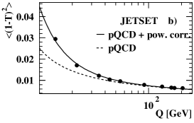
Figure 2: Results of fitting Eqs. (1,2,4) to Jetset predictions for mean values and higher moments of $1-T$.

Table 2: Results of fitting Eqs. (1,2,4) to Jetset predictions for mean values and higher moments of $1-T$.

$1-T$	Mean	2nd Moment	3rd Moment
$\alpha_{s}(M_{Z})$	0.108	0.1121	0.1131
$\bar{\alpha}_{n-1}$	0.380	1.34	5.7
$\chi^{2}/{\mathrm{ndf}}$	16	4.8	3.0

Another way of emphasising different ranges is to investigate higher moments. The OPAL Coll. investigated the power dependence of the first three moments of $1-T$ and the $C$-parameter $\!{}^{{\bf?}}$.

$$\left<f_{\mathrm{p}ow}\right>=a_{f}\frac{1}{n^{2}}\left(\frac{\mu_{I}}{E_{\mathrm{c}m}}\right)^{n}\left[\bar{\alpha}_{n-1}(\mu_{I})-\alpha_{s}(\mu)-\left(b_{0}\cdot\ln{\frac{\mu^{2}}{\mu_{I}^{2}}}+\frac{K}{2\pi}+\frac{2b_{0}}{n}\right)\alpha_{s}^{2}(\mu)\right]\quad{\rm,}$$ (4)

was used as power term. $\bar{\alpha}_{n-1}$ being a non-perturbative parameter accounting for the contributions to the event shape below an infrared matching scale $\mu_{I}$, $K=(67/18-\pi^{2}/6)C_{A}-5N_{f}/9$ and $a_{f}=4C_{f}/\pi$. Beside $\alpha_{s}$ these formulae contain $\bar{\alpha}_{n-1}$ as the only free parameters. The results shown for $\left<1-T\right>$ in Figure 2 and Table 2 indicate that the assumed power law of $1/E_{\mathrm{c}m}^{n}$ for the $n$-th moment does work.

3 Other Approaches

Figure 3: Fit results for cut variables (left), fitted 3rd order coefficient (middle) and fitted renormalisation scale (right). The continuous line represents the complete prediction. In the left plot the dashed line gives the perturbative contribution. In the middle plot it represents the 2nd order contribution to the full 3rd order curve.

To strengthen the need for power corrections in the description of data, a few other approaches were investigated: Fitting only the perturbative prediction including a 3rd order coefficient as free parameter yields very large $\chi^{2}$ and a 3rd order coefficient $C={\cal O}(1000)$ for $\left<1-T\right>$ and $\left<M^{2}_{\mathrm{h}}/E^{2}_{\mathrm{v}is}\right>$. Thus a 3rd order calculation does not give an improved prediction on the energy dependence neglecting hadronisation effects. (Figure 3b).

Leaving the renormalisation scale $x_{\mu}=\mu^{2}/E_{\mathrm{c}m}^{2}$ free, shows ambivalent results. While for $\left<1-T\right>$ the fit is reasonable and leads to a scale $x_{\mu}$ that is consistent with the one obtained from fits to distributions, the fit for $\left<M^{2}_{\mathrm{h}}/E^{2}_{\mathrm{v}is}\right>$ cannot describe the data. (Figure 3c).

To obtain the functional type of power corrections needed, one can also fit with an arbitrary power $p$:

$$\left<f_{\mathrm{p}ow}\right>=\frac{C_{p}}{E_{\mathrm{c}m}^{p}}$$ (5)

For $\left<1-T\right>$ one gets $p=0.98\pm 0.19$ $\!{}^{{\bf?}}$ in perfect agreement with the previous results.

4 Determination of $\alpha_{s}$ using Power Corrections

The analytical power ansatz for non-perturbative corrections by Dokshitzer and Webber $\!{}^{{\bf?},{\bf?}}$ is used by DELPHI to determine $\alpha_{s}$ from mean event shapes $\!{}^{{\bf?},{\bf?}}$. The power correction of this ansatz is given by

$$\left<f_{\mathrm{p}ow}\right>=a_{f}\cdot\frac{\mu_{I}}{E_{\mathrm{c}m}}\left[\bar{\alpha}_{0}(\mu_{I})-\alpha_{s}(\mu)-\left(b_{0}\cdot\ln{\frac{\mu^{2}}{\mu_{I}^{2}}}+\frac{K}{2\pi}+2b_{0}\right)\alpha_{s}^{2}(\mu)\right]\quad{\rm,}$$ (6)

with $\mu_{I}$, $K$, $a_{f}$ and $b_{0}$ as given above. In order to measure $\alpha_{s}$ from individual high energy data the free parameter $\bar{\alpha}_{0}$ has to be known.

Table 3: Determination of $\bar{\alpha}_{0}$. For $E_{\mathrm{c}m}\geq M_{Z}$ only DELPHI measurements are included in the fit. The first error is the statistical error from the fit, the second one is the scale error.

Observable	$\bar{\alpha}_{0}$	$\alpha_{s}(M_{Z})$	$\Lambda_{\overline{MS}}$[  MeV]	$\chi^{2}/\mathrm{ndf}$
$\left<1-T\right>$	$0.531\pm 0.012\pm 0.003$	$0.1187\pm 0.0017\pm 0.0060$	$235\pm 22\pm 70$	42/23
$\left<M_{h}^{2}/E_{\mathrm{v}is}^{2}\right>$	$0.434\pm 0.010\pm 0.010$	$0.1144\pm 0.0012\pm 0.0041$	$184\pm 13\pm 40$	4.0/14

To infer $\bar{\alpha}_{0}$ a combined fit of $\alpha_{s}$ and $\bar{\alpha}_{0}$ to a large set of measurements at different energies $\!{}^{{\bf?}}$ is performed. For $E_{\mathrm{c}m}\geq M_{Z}$ only DELPHI measurements are included in the fit. The resulting values of $\bar{\alpha}_{0}$ are summarised in Table 3. The extracted $\bar{\alpha}_{0}$ values are around 0.5 as expected in $\!{}^{{\bf?}}$. The numerical values are, however, incompatible with each other. So the assumed universality $\!{}^{{\bf?}}$ is not valid to the precision that is accessible from the data. Therefore $\bar{\alpha}_{0}$ is determined for $\left<1-T\right>$ and $\left<M_{h}^{2}/E_{\mathrm{v}is}^{2}\right>$ individually. The scale error is obtained from varying the renormalisation scale factor $x_{\mu}=\mu^{2}/E_{\mathrm{c}m}^{2}$ from 0.25 to 4 and the infrared matching scale from $1\mbox{\,\,Ge\kern-0.86108ptV}$ to $3\mbox{\,\,Ge\kern-0.86108ptV}$.

After having fixed $\bar{\alpha}_{0}$, the $\alpha_{s}$ values corresponding to the high energy data points can be calculated from Eqs. (1,2,6). $\alpha_{s}$ is calculated for both observables individually and then combined with an unweighted average. The resulting $\alpha_{s}$ values and the QCD expectation are shown in the leftmost plot of Figure 4.

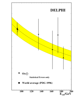
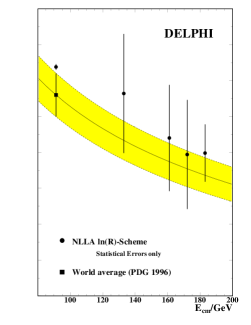
Figure 4: Energy dependence of $\alpha_{s}$ as obtained from mean event shapes (left) compared to $\alpha_{s}$ obtained from distributions. The errors shown are statistical only. The band shows the QCD expectation of extrapolating the world average to other energies.

Table 4: Running of $\alpha_{s}$ ($d\alpha/dE_{\mathrm{cm}}$) between 91  GeV and 183  GeV.

Means plus	Distributions plus
Power corr.	Monte Carlo based hadronisation models			QCD pred.
$\cal O$($\alpha_{s}^{2}$)	$\cal O$($\alpha_{s}^{2}$)	NLLA	$\cal O$($\alpha_{s}^{2}$)+NLLA
$-0.13\pm 0.05$	$-0.13\pm 0.05$	$-0.15\pm 0.05$	$-0.13\pm 0.04$	$-0.13\quad\cdot 10^{-3}\mbox{\,\,Ge\kern-0.86108ptV}^{-1}$

The $\alpha_{s}$ values follow the QCD expectation. Fitting a straight line to the energy dependence results in a slope, which agrees very well with the QCD expectation of a running $\alpha_{s}$ between 91  GeV and 183  GeV. In Figure 4 and Table 4 this result is further-on compared to $\alpha_{s}$ measurements obtained from distributions using Monte Carlo based hadronisation models. The comparison shows that the running measured from means using power correction and the one obtained from standard methods give consistent results and comparable errors.

5 Prospects

Many of the recent developments in the field of power corrections are not yet included in the presented experimental works. Beside the calculation of Milan factors, which will not influence the consistency of the experimental results much, some of the predicted power coefficients $a_{f}$ were corrected in the last months $\!{}^{{\bf?}}$. First tests show that the consistency of measured $\bar{\alpha}_{0}$ and $\alpha_{s}$ values improve with these new predictions.

Thus the experimental fits have to be repeated and with increasing theoretical understanding consistent experimental results hopefully will arise.

References

References

- [1] R. K. Ellis, D. A. Ross, and A. E. Terrano. Nucl. Phys B178(1981) 412.
- [2] CERN 89-08 Vol. 1, 1989.
- [3] ALEPH Coll. Phys. Lett. B284 (1992) 163; ALEPH Coll. Z. Phys. C55 (1992) 209; AMY Coll. Phys. Rev. Lett. 62 (1989) 1713; AMY Coll. Phys. Rev. D41 (1990) 2675; CELLO Coll. Z. Phys. C44 (1989) 63; HRS Coll. Phys. Rev. D31 (1985) 1; JADE Coll. Z. Phys. C25 (1984) 231; JADE Coll. Z. Phys. C33 (1986) 23; P.A. Movilla Fernandez, et. al. and the JADE Coll. Eur. Phys. J. C1 (1998) 461; L3 Coll. Z. Phys. C55 (1992) 39; Mark II Coll. Phys. Rev. D37 (1988) 1; Mark II Coll. Z. Phys. C43 (1989) 325; MARK J Coll. Phys. Rev. Lett. 43 (1979) 831; OPAL Coll. Z. Phys. C59 (1993) 1; PLUTO Coll. Z. Phys. C12 (1982) 297; SLD Coll. Phys. Rev. D51 (1995) 962; TASSO Coll. Phys. Lett. B214 (1988) 293; TASSO Coll. Z. Phys. C45 (1989) 11; TASSO Coll. Z. Phys. C47 (1990) 187; TOPAZ Coll. Phys. Lett. B227 (1989) 495; TOPAZ Coll. Phys. Lett. B278 (1992) 506; TOPAZ Coll. Phys. Lett. B313 (1993) 475.
- [4] L3 Coll. M. Acciarri et al. Phys. Lett. B411(1997) 339.
- [5] J. Drees, A. Grefrath, K. Hamacher, O. Passon, and D. Wicke. DELPHI 97-92 CONF 77, contributed to the EPS HEP conference in Jerusalem, 1997.
- [6] J. Drees, U. Flagmeyer, K. Hamacher, O. Passon, R. Reinhardt, and D. Wicke. DELPHI 98-18 CONF 119, contributed to Moriond, 1998.
- [7] OPAL Coll. OPAL PN 310, 1997.
- [8] ALEPH Coll. LP 258, Contributed to Lepton-Photon Conference, Hamburg, 1997.
- [9] Y. L. Dokshitzer and B. R. Webber. Phys. Lett. B352(1995) 451.
- [10] B. R. Webber. Talk given at workshop on DIS and QCD in Paris, hep-ph/9510283, 1995.
- [11] A. Lucenti and G. Salam. In these proceedings.