Three-body annihilation of neutralinos below two-body thresholds

Abstract:

We calculate the cross section for $s$-wave neutralino annihilation to three-body final states below the $W^{+}W^{-}$ and $t\bar{t}$ thresholds. Such three-body channels may dominate the annihilation cross section if the neutralino mass is not too much less than $m_{t}$ and $m_{W}$ respectively. Furthermore, because neutrinos produced in these channels are much more energetic than those from the $b\bar{b}$ or $\tau^{+}\tau^{-}$ channels, they can dominate the energetic-neutrino fluxes from neutralino annihilation in the Sun or Earth far below these thresholds and significantly enhance the neutrino signal in certain regions of the supersymmetric parameter space.

1 Introduction

It has long been well established that the observed luminous matter in Galactic halos cannot account for their total mass. Determination of the identity of this unseen dark matter has become one of the most important problems in modern cosmology. Perhaps the most promising dark-matter candidate is the neutralino $\chi$ [1], a linear combination of the supersymmetric partners of the $Z$, $\gamma$, and Higgs bosons.

The existence of neutralinos in our halo could be inferred by observation of energetic neutrinos from annihilation of neutralinos that have accumulated at the core of the Sun and/or Earth in detectors such as AMANDA, super-Kamiokande, MACRO, and HANUL [2]. These neutrinos are produced by decays of neutralino annihilation products such as $\tau$ leptons, $c$, $b$, and $t$ quarks, and gauge and Higgs bosons if the neutralino is heavy enough. In all cases where the signal is expected to be observable by these or subsequent-generation detectors, accretion of neutralinos from the Galactic halo onto the Sun or Earth comes into equilibrium with their depletion through annihilation [3]. Therefore, the annihilation rate depends on the rate of capture of neutralinos from the halo.

Although the total annihilation cross section is not needed for flux predictions, the branching ratios into the various annihilation products are: The rate for observation of neutrinos from decays of various annihilation products may differ considerably. Energetic neutrinos are much more easier to detect than low-energy ones. For example, the flux of energetic neutrinos from decays of $b$ quarks is much smaller than that from gauge bosons or top quarks with the same injection energy.

The best technique for inferring the existence of these neutrinos is to observe an upward muon produced by a charged-current interaction in the rock below the detector. The rate for observation of energetic neutrinos is proportional to the second moment of the neutrino energy spectrum, so it is this neutrino energy moment weighted by the corresponding branching ratio that determines the detection rate.

By now, the cross sections for annihilation have been calculated for all two-body final states that arise at tree level (fermion-antifermion and gauge- and Higgs-boson pairs). The precise branching ratios depend on numerous coupling constants and superpartner masses. However, roughly speaking, among the two-body channels the $b\bar{b}$ and $\tau^{+}\tau^{-}$ final states usually dominate for $m_{\chi}<m_{W}$. Neutralinos that are mostly higgsino annihilate primarily to gauge bosons if $m_{\chi}>m_{W}$, because there is no $s$-wave suppression mechanism for this channel. Neutralinos that are mostly gaugino continue to annihilate primarily to $b\bar{b}$ pairs until the neutralino mass exceeds the top-quark mass, after which the $t\bar{t}$ final state dominates, as the cross section for annihilation to fermions is proportional to the square of the fermion mass.

Three-body final states arise only at higher order in perturbation theory and are therefore usually negligible. However, as we already noted, some two-body channels easily dominates the cross section when they are open because of their large couplings, for example the $W^{+}W^{-}$ for the higgsinos and $t\bar{t}$ for gauginos. This suggests that their corresponding three-body final states can be important just below these thresholds.

More importantly, as mentioned above, the rate for indirect detection is also proportional to the second moment of the energy of the muon neutrino. The neutrinos produced in these three-body final states are generally much more energetic than those produced in $b$ and $\tau$ decays, so even when the cross sections to these channels are small compared with others, they could dominate the indirect-detection rate.

In this paper, we calculate the cross section for the processes $\chi\chi\to W^{+}W^{-*}\to Wf\bar{f^{\prime}}$ and $\chi\chi\rightarrow t\bar{t}^{*}\rightarrow tW^{-}\bar{b}$, and their charge conjugates (heretofore referred as $tWb$ and $WW^{*}$ states) in the $v_{\rm rel}\to 0$ limit, where the star denotes virtual particles. Our calculation for the $WW^{*}$ is applicable for generic neutralinos, but it is mostly significant for neutralinos that are primarily made of higgsino. This is because the gauginos have small couplings to $W^{+}W^{-}$ pairs. As for the $tWb$ final state, our calculation is only applicable to the gaugino. If the neutralino is primarily higgsino, then annihilation to this final state could also proceed through a $WW^{*}$ intermediate state, which we have not included in our calculation. However, if the neutralino is primarily higgsino with $m_{W}<m_{\chi}<m_{t}$, then it will annihilate primarily to $W^{+}W^{-}$ pairs below the $t\bar{t}$ threshold. Furthermore, the neutrino yield from $W^{+}W^{-}$ pairs is similar to that for $t\bar{t}$ pairs. Therefore, neutrino rates are affected only weakly if the process $\chi\chi\to WW^{*}\to tWb$ is neglected.

Annihilation in the Sun and Earth takes place only when the annihilating neutralinos have relative velocities $v\sim 10^{-3}\ll 1$. Therefore, if we expand the annihilation cross section as

$$\sigma v=a+bv^{2}\,,$$ (1)

then we consider only the $a$ (the $s$-wave) term. The relic abundance also depends on the annihilation cross section. However, annihilation in the early Universe takes place when $v\sim 0.5$. In the early Universe, thermal averaging of the cross section smoothes out the jump in the annihilation rate near particle thresholds [4]. Therefore, three-body final states should have only a negligible effect on the relic abundance, so we do not consider it further.

We calculate the cross section and neutrino signal for the $tt^{*}$ final state in Section II and those for the $WW^{*}$ final state in Section III, and discuss these results in Section IV. Some lengthy matrix elements needed for the calculation are given in the Appendices.

2 Calculation of the $tWb$ final state

Figure 1: Feynman diagrams for annihilation of neutralinos to the $tW^{-}\bar{b}$ final state through an intermediate $t\bar{t}^{*}$ state.

We begin by calculating the cross section to the $tWb$ final state. In some respects, our calculation parallels a recent calculation of the three-body decay of Higgs bosons into this final state [5]. The Feynman diagrams for this process are shown in Fig. 1. Like annihilation to $t\bar{t}$ pairs, annihilation to this three-body final state takes place via $s$-channel exchange of $Z^{0}$ and $A^{0}$ (pseudo-scalar Higgs) and $t$- and $u$-channel exchange of squarks. Although there are additional diagrams for this process, such as those shown in Fig. 2, these are negligible for the regions of parameter space that we investigate for the reasons discussed in the Introduction.

Figure 2: The contribution to the $tWb$ final state from $W^{+}W^{-}$ pairs. These are negligible for the regions of parameter space we investigate.

The total cross section for annihilation into three-body final states is given by [6]

$$\sigma=\int\frac{N_{c}}{2(2\pi)^{5}\lambda^{1/2}(s,m_{\chi}^{2},m_{\chi}^{2})}\frac{1}{4}|{\mathcal{M}}|^{2}d_{3}PS\,;$$ (2)

where

$$\lambda(x,y,z)=x^{2}+y^{2}+z^{2}-2xy-2yz-2zx\,;$$ (3)

${\cal M}$ is the matrix element for the process; $N_{c}$ is the color factor; and $d_{3}PS$ is the three-body phase space which can be written as

$$d_{3}PS = \int\delta^{4}(p_{1}+p_{2}-p_{4}-p_{5}-p_{6})\frac{d^{3}p_{4}}{2p_{4}^{0}}\frac{d^{3}p_{5}}{2p_{5}^{0}}\frac{d^{3}p_{6}}{2p_{6}^{0}}$$ (4)

$$= \frac{\pi^{2}s}{4}dx_{4}dx_{6}\,.$$

Here

$$x_{4}=\frac{2p_{4}^{0}}{\sqrt{s}}\,;\;\;\;\;\;\;\;\;x_{5}=\frac{2p_{5}^{0}}{\sqrt{s}}\,;\;\;\;\;\;\;\;\;x_{6}=\frac{2p_{6}^{0}}{\sqrt{s}}\,;$$ (5)

$p_{4}$, $p_{5}$, and $p_{6}$ are the four-momenta of the $t$ quark, $W$ boson and $\bar{b}$ quarks respectively, as shown in the Feynman diagrams; and $\sqrt{s}$ is the total center-of-mass energy. We approximate $m_{b}=0$, and take the $v_{\rm rel}\to 0$ limit where $v_{\rm rel}$ is the relative velocity of the annihilating neutralinos. The boundaries of the phase space are given by

$$x_{6\rm min} = 0;$$ (6)

$$x_{6\rm max} = 1-\frac{(m_{t}+m_{W})^{2}}{4m_{\chi}^{2}};$$ (7)

$$x_{4\rm min} = \frac{1}{2(1-x_{6})}\left[(2-x_{6})\left(1+\frac{m_{t}^{2}}{4m_{\chi}^{2}}-\frac{m_{W}^{2}}{4m_{\chi}^{2}}-x_{6}\right)\right.$$ (8)

$$\left.-x_{6}\lambda^{1/2}\left(1-x_{6},\frac{m_{t}^{2}}{4m_{\chi}^{2}},\frac{m_{W}^{2}}{4m_{\chi}^{2}}\right)\right];$$

$$x_{4\rm max} = \frac{1}{2(1-x_{6})}\left[(2-x_{6})\left(1+\frac{m_{t}^{2}}{4m_{\chi}^{2}}-\frac{m_{W}^{2}}{4m_{\chi}^{2}}-x_{6}\right)\right.$$ (9)

$$\left.+x_{6}\lambda^{1/2}\left(1-x_{6},\frac{m_{t}^{2}}{4m_{\chi}^{2}},\frac{m_{W}^{2}}{4m_{\chi}^{2}}\right)\right].$$

The total cross section is then given by

$$\sigma v_{\rm rel}=\frac{N_{c}}{128\pi^{3}}\int_{x_{6min}}^{x_{6max}}dx_{6}\int_{x_{4min}}^{x_{4max}}dx_{4}\frac{1}{4}|{\cal M}|^{2}\,,$$ (10)

where the spin-summed amplitude squared is given by:

$$|{\cal M}|^{2}=\sum_{{\rm spin}}|M|^{2}\,,$$ (11)

with

$$M=M_{1t}+M_{2t}+M_{3t}+M_{4t}-M_{1u}-M_{2u}-M_{3u}-M_{4u}+M_{5}+M_{7}\,.$$ (12)

If we make the approximation $t,u\ll m_{\tilde{f}}^{2}$ (we cannot make this approximation for $s$ in this case), then the $M_{i}$s are given by

$$M_{1t} = \frac{g}{\sqrt{2}}c_{1}\bar{u_{6}}\gamma_{\mu}L\epsilon_{5}^{\mu}\frac{1}{p\!\!\!/_{3}-m_{t}}Lu_{1}\bar{v_{2}}Rv_{4}\,;\qquad M_{1u}=\frac{g}{\sqrt{2}}c_{1}\bar{u_{6}}\gamma_{\mu}L\epsilon_{5}^{\mu}\frac{1}{p\!\!\!/_{3}-m_{t}}Lu_{2}\bar{v_{1}}Rv_{4}\,;$$

$$M_{2t} = \frac{g}{\sqrt{2}}c_{2}\bar{u_{6}}\gamma_{\mu}L\epsilon_{5}^{\mu}\frac{1}{p\!\!\!/_{3}-m_{t}}Ru_{1}\bar{v_{2}}Lv_{4}\,;\qquad M_{2u}=\frac{g}{\sqrt{2}}c_{2}\bar{u_{6}}\gamma_{\mu}L\epsilon_{5}^{\mu}\frac{1}{p\!\!\!/_{3}-m_{t}}Ru_{2}\bar{v_{1}}Lv_{4}\,;$$

$$M_{3t} = \frac{g}{\sqrt{2}}c_{3}\bar{u_{6}}\gamma_{\mu}L\epsilon_{5}^{\mu}\frac{1}{p\!\!\!/_{3}-m_{t}}Lu_{1}\bar{v_{2}}Lv_{4}\,;\qquad M_{3u}=\frac{g}{\sqrt{2}}c_{3}\bar{u_{6}}\gamma_{\mu}L\epsilon_{5}^{\mu}\frac{1}{p\!\!\!/_{3}-m_{t}}Lu_{2}\bar{v_{1}}Lv_{4}\,;$$

$$M_{4t} = \frac{g}{\sqrt{2}}c_{4}\bar{u_{6}}\gamma_{\mu}L\epsilon_{5}^{\mu}\frac{1}{p\!\!\!/_{3}-m_{t}}Ru_{1}\bar{v_{2}}Rv_{4}\,;\qquad M_{4u}=\frac{g}{\sqrt{2}}c_{4}\bar{u_{6}}\gamma_{\mu}L\epsilon_{5}^{\mu}\frac{1}{p\!\!\!/_{3}-m_{t}}Ru_{2}\bar{v_{1}}Rv_{4}\,;$$

and

$$M_{5} = \frac{g}{\sqrt{2}}\bar{u_{6}}\gamma_{\mu}L\epsilon_{5}^{\mu}\frac{1}{p\!\!\!/_{3}-m_{t}}(c_{5}R+c_{6}L)\gamma^{\nu}v_{4}\bar{v_{2}}\gamma_{\nu}\gamma_{5}u_{1}\,;$$

$$M_{7} = \frac{g}{\sqrt{2}}c_{7}\bar{u_{6}}\gamma_{\mu}L\epsilon_{5}^{\mu}\frac{1}{p\!\!\!/_{3}-m_{t}}\gamma_{5}v_{4}\bar{v_{2}}\gamma_{5}u_{1}\,.$$

Here, the subscripts 4,5,6 denotes the $t(\bar{t})$, $W^{-}$($W^{+}$) and $\bar{b}$($b$) respectively, and $p_{3}=p_{5}+p_{6}$ is the 4-momentum of the virtual top quark. The subscript $t$ and $u$ denotes $t$- and $u$-channel exchange of a sfermion. The left- and right-hand projectors $L$ and $R$ are

$$R=\frac{1+\gamma_{5}}{2},\qquad L=\frac{1-\gamma_{5}}{2}\,;$$ (13)

and the coefficients $c_{i}$ are given by

$$c_{1} = \sum_{j=1}^{6}\frac{1}{m_{\tilde{f_{j}}}^{2}}W_{j}^{{}^{\prime}2}\,;\qquad c_{2}=\sum_{j=1}^{6}\frac{1}{m_{\tilde{f_{j}}}^{2}}X_{j}^{{}^{\prime}2}\,;\qquad c_{3}=c_{4}=\sum_{j=1}^{6}\frac{1}{m_{\tilde{f_{j}}}^{2}}W^{\prime}_{j}X^{\prime}_{j};$$

$$c_{5} = \frac{2g^{2}c_{r}(N_{30}^{2}-N_{40}^{2})}{s\cos^{2}\theta_{w}-4m_{W}^{2}}\,;\;\;c_{6}=\frac{2g^{2}c_{l}(N_{30}^{2}-N_{40}^{2})}{s\cos^{2}\theta_{w}-4m_{W}^{2}}\,;\;\;c_{7}=\frac{2gT_{A00}h_{Aff}}{s-2m_{A}^{2}}\,;$$

where the sum on $j$ is over the squarks; $j=1,2,3$ for left-handed squarks and $j=4,5,6$ for right-handed squarks. The quantities $m_{\tilde{f_{j}}}$ are the masses of sfermions $j$. The couplings $W^{\prime}_{j}$ and $X^{\prime}_{j}$ are $\chi f\tilde{f}$ right-hand and left-hand couplings respectively; they are defined as $W^{\prime}_{u,t,j,0}$ and $X^{\prime}_{u,t,j,0}$ in the notation of [1], and $T_{A00}$ and $h_{Aff}$ are couplings of the Higgs boson $A$. $N_{30}$ and $N_{40}$ are the composition coefficients of the neutralino given in [1]. Also,

$$c_{l}=\frac{1}{2}-\frac{2}{3}\sin^{2}\theta_{W}\,;\;\;\;\;\;\;\;\;c_{r}=-\frac{2}{3}\sin^{2}\theta_{W}\,.$$ (14)

For the virtual-top propagator we use the relativistic Wigner-Weisskopf form

$$\frac{p\!\!\!/_{3}+m_{t}}{p_{3}^{2}-m_{t}^{2}+im_{t}\Gamma_{t}}\,.$$ (15)

The decay width of the top quark is not yet measured, so we use the prediction of the standard model,

$$\Gamma_{t}=\frac{G_{f}m_{t}^{3}}{8\pi\sqrt{2}}\left(1-\frac{m_{W}^{2}}{m_{t}^{2}}\right)^{2}\left(1+2\frac{m_{W}^{2}}{m_{t}^{2}}\right).$$ (16)

We calculate $|{\cal M}|^{2}$ using standard trace techniques. Notice also that

$$M_{it,jt}=M_{iu,ju}\equiv M_{i,j}\,,\;\;M_{5,it}=-M_{5,iu}\equiv M_{5,i}\,,\;\;M_{7,it}=-M_{7,iu}\equiv M_{7,i}\,;$$ (17)

where $i,j=1,2,3,4$. Thus, we have

$$|{\cal M}|^{2}= 2\left[M_{1,1}+M_{2,2}+M_{3,3}+M_{4,4}+2(M_{1,2}+M_{1,3}+M_{1,4}+M_{2,3}+M_{2,4}+M_{3,4})\right]$$ (18)

$$-2\left[M_{1t,1u}+M_{2t,2u}+M_{3t,3u}+M_{4t,4u}\right]+M_{5,5}+M_{7,7}$$

$$-4\left[M_{1t,2u}+M_{1t,3u}+M_{1t,4u}+M_{2t,3u}+M_{2t,4u}+M_{3t,4u}\right]$$

$$+4\left[M_{5,1}+M_{5,2}+M_{5,3}+M_{5,4}+M_{7,1}+M_{7,2}+M_{7,3}+M_{7,4}\right].$$

These $M_{i,j}$ are given in Appendix A.

Table 1: Model parameters for Fig. 3

$M_{2}=260-400$ GeV	$\mu=10^{4}$ GeV	$m_{A}=10^{3}$ GeV
$\tan\beta=2$	$m_{\tilde{q}}^{2}=10^{6}{\rm GeV}^{2}$	$m_{\tilde{l}}^{2}=10^{6}{\rm GeV}^{2}$

The three-body cross section for a series of typical models are shown in Fig. 3. The parameters of the models are given in Table  1. Here we assume the GUT mass relation $M_{1}=\frac{5}{3}M_{2}\tan^{2}\theta_{W}$, and the mass of the lightest neutralino varies as $M_{2}$ varies. Note that our choice of the parameter $\mu\gg M_{2}$ ensures that the neutralino is primarily gaugino. We have also chosen diagonal and degenerate mass matrices for the squarks and sleptons.

As expected, the three-body cross section approaches to the two-body value above the top threshold (we take $m_{t}=180$ GeV). Below the top mass it is non-zero but drops quickly.

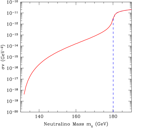
Figure 3: The dashed curve is the total annihilation cross section times relative velocity to two-body final states. The solid curve includes the $tWb$ final state as well.

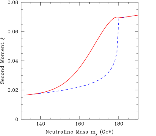
Figure 4: Detection rate of neutrinos from neutralino annihilation in the Earth versus neutralino mass. The ordinate is $\xi$ defined in Eqs.  (21) to which the detection rate is proportional. The dashed curve includes only two-body final states, the solid curve includes the $tWb$ final state as well.

We now consider the neutrino spectrum. If the rate for neutralino capture in the Sun is fixed, the flux of upward muon induced by energetic neutrinos from neutralino annihilation in the Sun and/or Earth depends on the various neutralino annihilation branching ratios, but not on the total annihilation cross section. The flux of upward muons (the quantity to be compared with experiment) is [1]

$$\Gamma_{\rm detect}\propto\xi_{\rm total}\equiv\sum_{i}a_{i}b_{i}\sum_{F}B_{F}{\left\langle Nz^{2}\right\rangle}_{F,i}(m_{\chi})\,,$$ (19)

where the sum on $i$ is over muon neutrinos and anti-neutrinos; $a_{i}$ are neutrino scattering coefficients, $a_{\nu}=6.8$ and $a_{\bar{\nu}}=3.1$; and $b_{i}$ are muon-range coefficients, $b_{\nu}=0.51$ and $b_{\bar{\nu}}=0.67$ [7]. The sum on $F$ is over all annihilation channels. The quantity $z=E_{\nu}/m_{\chi}$ is the neutrino energy scaled by the neutralino mass. In the two-body case, this is the same as the injection energy of the particle produced in neutralino annihilation, and the second moment is given by

$${\left\langle Nz^{2}\right\rangle}_{F,i}(E_{\rm in})\equiv\frac{1}{E_{\rm in}^{2}}\int\left(\frac{dN}{dE}\right)_{F,i}(E_{\nu},E_{\rm in})~{}E_{\nu}^{2}~{}dE_{\nu}\,.$$ (20)

The functions ${\left\langle Nz^{2}\right\rangle}_{F,i}(E_{\rm in})$ have been calculated for injection of all particles that the neutralino may annihilate to in both the Sun and Earth for both muon neutrinos and anti-neutrinos [7, 8]. Note that the ${\left\langle Nz^{2}\right\rangle}$ are different for particles injected in the Sun and Earth since slowing of quarks and slowing and absorption of neutrinos may be significant in the Sun but not in the Earth. For the same reason, the ${\left\langle Nz^{2}\right\rangle}$ for muon neutrinos and anti-neutrinos will differ for particles injected into the Sun, although they are the same for particles injected into the Earth.

In the three-body case, $E_{\rm in}\neq m_{\chi}$. However, Eqs. (20) can be generalized. For the $twb$ final state, the second moment is given by

$$B_{F}{\left\langle Nz^{2}\right\rangle}=\frac{3}{128\pi^{3}}\int dx_{4}dx_{6}|{\cal M}|^{2}\left({\left\langle Nz^{2}\right\rangle}_{t}x_{4}^{2}+{\left\langle Nz^{2}\right\rangle}_{W}x_{5}^{2}+{\left\langle Nz^{2}\right\rangle}_{b}x_{6}^{2}\right).$$ (21)

We plot the result for annihilation in the Earth in Fig. 4. (The results for annihilation in the Sun are similar.) We plot the relevant combination of the second moments ${\left\langle Nz^{2}\right\rangle}$ given in Eq. (19). The predicted muon flux is proportional to this quantity. The dashed curves in the Figure show the results obtained by ignoring the $tWb$ final state, and the solid curves show the results with the $tWb$ final state.

Although the three-body cross section is small except just below the $t\bar{t}$ threshold, its contribution to the the second moment $B_{F}{\left\langle Nz^{2}\right\rangle}$ may be important, as illustrated in Fig.  4. This is because the ${\left\langle Nz^{2}\right\rangle}$ for top quarks and $W$ bosons is significantly larger than that for the light fermions [8].

3 Neutralino annihilation to $WW^{*}$

Below the $W^{+}W^{-}$ threshold, the neutralino can annihilate to a real $W$ and a virtual $W$ which we denote by $W^{*}$. The real and virtual $W$ bosons then decay independently. About 10% of these decay into a muon (or anti-muon) and a muon anti-neutrino (or neutrino). These processes are illustrated in Fig. 5, where the $W^{*}$ decays into a fermion pair $f\bar{f^{\prime}}$, and the fermion pair can be $\tau\nu$, $\mu\nu$, $e\nu$, $cs$, or $ud$.

The $WW^{*}$ calculation is similar to the $tWb$ calculation. We are only interested in the $v\to 0$ limit. In this limit, only chargino exchange in the $t$ and $u$ channels shown in Fig. 5 are important. Neutrinos can be produced either by the virtual $W^{*}$ or by decay of the real $W$.

Figure 5: Neutralino annihilation to $Wf\bar{f}$ through a virtual $W^{*}$ by chargino exchange in the $t$ or $u$ channel.

The cross section is given again by Eq. (10), and $x_{4}$, $x_{5}$, and $x_{6}$ are defined similarly. Neglecting the fermion mass, the boundaries of the phase space can be written as:

$$x_{4\rm min} = \frac{m_{4}}{m_{\chi}},$$ (22)

$$x_{4\rm max} = 1+\frac{m_{4}^{2}}{4m_{\chi}^{2}},$$ (23)

$$x_{6\rm min} = \frac{1}{2}\left(2-x_{4}-\sqrt{x_{4}^{2}-\frac{m_{4}^{2}}{m_{\chi}^{2}}}\right),$$ (24)

$$x_{6\rm max} = \frac{1}{2}\left(2-x_{4}+\sqrt{x_{4}^{2}-\frac{m_{4}^{2}}{m_{\chi}^{2}}}\right).$$ (25)

where $m_{4}=m_{W}$. The amplitude is

$$M=M_{0t}+M_{1t}-M_{0u}-M_{1u}\,,$$ (26)

where

$$M_{i,t} = \frac{g^{2}}{k^{2}-m_{\chi^{+}_{i}}^{2}}\bar{v}_{2}\gamma^{\nu}(O_{i,L}^{2}L+O_{i,R}^{2}R)k\!\!\!/\gamma^{\mu}u_{1}W_{4\nu}W_{3\mu}\,,$$ (27)

$$M_{i,u} = \frac{g^{2}}{k^{{}^{\prime}2}-m_{\chi^{+}_{i}}^{2}}\bar{v}_{1}\gamma^{\nu}(O_{i,L}^{2}L+O_{i,R}^{2}R)k\!\!\!/^{{}^{\prime}}\gamma^{\mu}u_{2}W_{4\nu}W_{3\mu}\,.$$ (28)

Here $i=0,1$ denotes the two chargino states, $m_{\chi^{+}_{i}}$ their masses, and $O_{i,L}$ and $O_{i,R}$ are the couplings. The quantity $k=p_{4}-p_{2}$ and $k^{\prime}=p_{4}-p_{1}$ are the momentum transfered in the $t$ and $u$ channel respectively, and in the $v\to 0$ limit, $p_{1}=p_{2}$ and $k=k^{\prime}$. Also,

$$W_{3\mu}=\frac{g}{\sqrt{2}}\frac{1}{p_{3}^{2}-m_{W}^{2}+im_{W}\Gamma_{W}}\bar{u_{5}}\gamma_{\mu}Lu_{1}\,,$$ (29)

and $W_{4\nu}$ is the wavefunction for the outgoing $W$ boson.

Straightforward calculation yields

$$|{\cal M}|^{2}=Ng^{4} \left\{{\displaystyle\sum_{i=0}^{1}}\frac{2}{(k^{2}-M_{i}^{2})^{2}}\left[\left(O_{iL}^{4}+O_{iR}^{4}\right)M_{tta}+2O_{iL}^{2}O_{iR}^{2}M_{ttb}\right]\right.$$

$$\left.+\frac{4}{(k^{2}-M_{0}^{2})(k^{2}-M_{1}^{2})}\left[\left(O_{0L}^{2}O_{1L}^{2}+O_{0R}^{2}O_{1R}^{2}\right)\left(M_{tta}-M_{tua}\right)\right.\right.$$

$$\left.\left.+\left(O_{0L}^{2}O_{1R}^{2}+O_{0R}^{2}O_{1L}^{2}\right)\left(M_{ttb}-M_{tub}\right)\right]\right.$$

$$\left.-{\displaystyle\sum_{i=0}^{1}}\frac{2}{(k^{2}-M_{i}^{2})^{2}}\left[\left(O_{iL}^{4}+O_{iR}^{4}\right)M_{tua}+2O_{iL}^{2}O_{iR}^{2}M_{tub}\right]\right\},$$

where

$$N=\frac{g^{2}(p_{5}p_{6})}{(p_{3}^{2}-m_{W}^{2})^{2}+m_{W}^{2}\Gamma_{W}^{2}}\,,$$ (30)

and the matrix elements $M_{i,j}$ are listed in Appendix B.

This cross section can be evaluated numerically. The result for models with parameters given in Table 2 is shown in Fig. 6. Like the $twb$ case, the three-body annihilation cross section drops quickly below $m_{W}$ and approaches zero as $m_{\chi}\to m_{W}/2$.

$M_{2}=1000$ GeV	$\mu=55-110$ GeV	$m_{A}=1000$ GeV
$\tan\beta=2$	$m_{\tilde{q}}^{2}=10^{10}{\rm GeV}^{2}$	$m_{\tilde{l}}^{2}=10^{10}{\rm GeV}^{2}$

Table 2: Model parameters for Fig. 6.

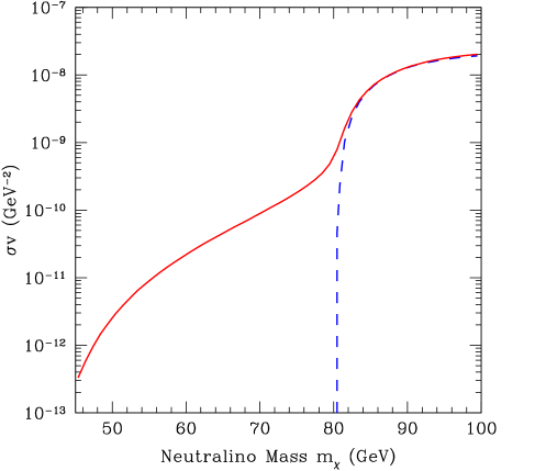
Figure 6: Cross section times relative velocity for neutralino annihilation to $W\mu\nu$. The dashed curve includes only two-body final states and the solid curve includes the three-body final states.

The calculation of neutrino flux is again analogous to the $twb$ case. However, we will not consider the neutrinos produced by decay of the muon or other fermions as they are of negligibly low energy. We have

$$B_{F}{\left\langle Nz^{2}\right\rangle}=\frac{1}{128\pi^{3}}\int dx_{4}dx_{6}|{\cal M}|^{2}\left(\frac{1}{4}(1+\frac{2}{5}\beta_{W}^{2})x_{4}^{2}+x_{6}^{2}\right)/2\,,$$ (31)

where $\beta_{W}$ is the velocity of the real $W$ boson. The second term on the right-hand side accounts for the neutrino produced via the $W^{*}$. The first term is from the decay of the real $W$ boson. This $W$ boson has a probability of $\Gamma_{W\to\mu\nu}$ to decay to a muon neutrino. On the other hand this $W$ boson is produced in all $\chi\chi\to Wf\bar{f^{\prime}}$ channels, and each of these channels has approximately the same cross section, so the contribution has a weight of $n_{chan}\Gamma_{W\to\mu\nu}\approx 1$.

The result for annihilation in the Earth is shown in Fig. 7. The results for annihilation in the Sun look similar. We see again the second moment agrees with the $WW$ result above the threshold, but does not decrease immediately below $m_{W}$, despite the fast drop of the cross section. In fact, the value of the second moment is slightly higher below the $WW$ threshold, and does not drop until the cross section vanishes as $m_{\chi}$ approaches $m_{W}/2$. Below $m_{W}/2$, the four-body channel might become significant, and may smooth the jump in much the same fashion as the three-body channel does near the two-body channel threshold, but we will not consider it here.

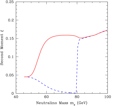
Figure 7: Second moment $\xi$ of neutrino energy spectrum for neutrinos from neutralino annihilation in the Earth. The dashed curve is the two-body calculation, and the solid curve includes the three-body final states from an intermediate $WW^{*}$ state as well.

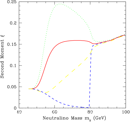
Figure 8: Contributions to the second moment $\xi$ for annihilations in the Earth. Short dashed curve: two-body result; solid curve: three-body result; dotted curve: (twice of) real $W$ contribution; long dashed curve: (twice of) virtual $W^{*}$ contribution.

To understand why there is a dip near the $WW$ threshold in Fig. 7, consider Eq. (31). There are two terms in the integrand. The $x_{4}^{2}$ term is the contribution from the decay of the “on-shell” $W$, and the $x_{6}^{2}$ term is from the virtual $W^{*}$. We plot these contributions separately in Fig. 8.

To make comparison easier, what are actually plotted are twice the contributions from these terms plus contribution from other channels. As one can see from the plot, both the real and virtual $W$ contributions agree with the two-body result above the threshold as expected; below the threshold, however, their behaviors are quite different. While the virtual $W^{*}$ contribution smoothly drops, the real $W$ contribution actually peaks well below the threshold; then it decreases as $m_{\chi}$ increases, and has a sharp turn at the $WW$ threshold. This is because the the second moment is proportional to $x_{4}^{2}$, and below the threshold $x_{4}$ steadily decreases as $m_{\chi}$ increases, as can be seen from Eqs. (22)–(23). However, above the threshold, $x_{4}$ is stabilized at the $x_{4}=1$ pole, so it stops decreasing, and gradually increases as $\beta_{W}$ increases. When averaged with the smooth curve of the $W^{*}$ contribution, this produces the strange dip at the threshold.

In this calculation we have assumed that one $W$ is on-shell while the other is off-shell. It could happen that both $W$’s are off-shell, and if such contributions are important this may produce a smoother curve and the dips in these plots may disappear. We examined this possibility by smearing the on-shell mass $m_{4}$ in the range $m_{W}-3\Gamma_{W}<m_{4}<m_{W}+3\Gamma_{W}$ and calculating an average with the assumption that the cross section is proportional to

$$\frac{1}{(m_{4}^{2}-m_{W}^{2})^{2}-m_{W}^{2}\Gamma_{W}^{2}}.$$

This produces a result that differs by less than $10^{-4}$ from the simple on-shell result. Hence it suggests that the on-shell approximation works well.

4 Conclusions

We made several approximations in our calculation. For example, in the $tWb$ calculation, we neglected the contributions from diagrams involving production of the $tWb$ final state through virtual $W$ bosons. However, in those regions of parameter space where such omissions become unacceptable, the process we are considering is not very important. In the $Wf\bar{f^{\prime}}$ case, our calculation is generally applicable, but it is most useful for a higgsino, since in that case the $W^{+}W^{-}$ channel becomes large above threshold.

Although the contributions of these three-body channels are important only in a limited region of parameter space, it may be a large effect. In fact, our calculation shows that although the cross sections of these annihilations are significant only just below the two-body channel threshold, due to the high energy of the neutrinos they produce, they can enhance the neutrino signal by many times and actually dominate the neutrino signal far below the two-body threshold. Furthermore, the regions in question may be of particular interest. For example, motivated by collider data, Kane and Wells proposed a light higgsino [9] (but see [10]). There are also arguments that the neutralino should be primarily gaugino with a mass somewhere below but near the top-quark mass [11].

There are many parameters in the minimal supersymmetric model. The results shown in Figs. 4 and 7 are of course model dependent, and these effects might be more or less important in models with different parameters. For a generic neutralino, these effects would be small. However, for the regions of parameter spaces we have focussed on it seems that the increase of the indirect-detection rate is fairly robust. For these regions of parameter space these effects should be considered for calculations of rates for energetic-neutrino detection.

Appendix A The $tt^{*}$ cross section

We give the $M_{i,j}$ for the $tt^{*}$ cross section calculation in this Appendix.

For convenience, we introduce four-momenta

$$a=-\left[b-\frac{2(p_{3}b)}{p_{3}^{2}}p_{3}\right],\;\;\;\;b=p_{6}+\frac{2(p_{5}p_{6})}{m_{W}^{2}}p_{5}\,,$$ (32)

[these should not be confused with the cross-section factors introduced in Eq. (1)]. We further introduce

$$N=\frac{1}{2}\frac{g^{2}}{(p_{3}^{2}-m_{t}^{2})^{2}+\Gamma_{t}^{2}m_{t}^{2}}\,.$$ (33)

We can then write the $M_{i,i}$ as

$$M_{1,1} = 4Nc_{1}^{2}m_{t}^{2}(p_{1}b)(p_{2}p_{4})\,,\qquad M_{2,2}=4Nc_{2}^{2}p_{3}^{2}(p_{1}a)(p_{2}p_{4})\,,$$

$$M_{3,3} = 4Nc_{3}^{2}m_{t}^{2}(p_{1}b)(p_{2}p_{4})\,,\qquad M_{4,4}=4Nc_{4}^{2}p_{3}^{2}(p_{1}a)(p_{2}p_{4})\,,$$

and

$$M_{5,5}= 16N \left\{c_{5}^{2}p_{3}^{2}\left[(p_{1}p_{4})(p_{2}a)+(p_{1}a)(p_{2}p_{4})-m_{\chi}^{2}(p_{4}a)\right]\right.$$

$$\left.+c_{6}^{2}m_{3}^{2}\left[(p_{1}p_{4})(p_{2}b)+(p_{1}b)(p_{2}p_{4})-m_{\chi}^{2}(p_{4}b)\right]\right.$$

$$\left.+2c_{5}c_{6}m_{t}^{2}(p_{3}b)\left((p_{1}p_{2})-2m_{\chi}^{2})\right)\right\},$$

$$M_{7,7}= 16N c_{7}^{2}m_{\chi}^{2}\left\{2\left[(p_{3}p_{4})+m_{t}^{2}\right](p_{3}b)+\left[m_{t}^{2}-p_{3}^{2}\right](p_{4}b)\right\}.$$

The $M_{i,j}$’s are given by

$$M_{1,2} = 4Nc_{1}c_{2}m_{\chi}^{2}m_{t}^{2}(p_{3}b)\,,\qquad\qquad\;\;M_{1,3}=4Nc_{1}c_{3}m_{\chi}m_{t}^{3}(p_{1}b)\,,$$

$$M_{1,4} = 4Nc_{1}c_{4}m_{\chi}m_{t}(p_{3}b)(p_{2}p_{4})\,,\qquad M_{2,3}=4Nc_{2}c_{3}m_{\chi}m_{t}(p_{3}b)(p_{2}p_{4})\,,$$

$$M_{2,4} = 4Nc_{2}c_{4}m_{\chi}m_{t}(p_{3}p_{3})(p_{1}a)\,,\qquad M_{3,4}=4Nc_{3}c_{4}m_{\chi}^{2}m_{t}^{2}(p_{3}b)\,,$$

and

$$\begin{split}M_{5,1}=-4Nc_{1}m_{t}^{2}&\left\{c_{5}\left[(p_{1}p_{2})(p_{3}b)+(p_{2}p_{3})(p_{1}b)-(p_{1}p_{3})(p_{2}b)-2m_{\chi}^{2}(p_{3}b)\right]\right.\\ &\left.+c_{6}\left[2(p_{2}p_{4})(p_{1}b)-m_{\chi}^{2}(p_{4}b)\right]\right\},\end{split}$$

$$\begin{split}M_{5,2}=&4Nc_{2}\left\{c_{5}\left[4(p_{2}p_{4})(p_{1}p_{3})(p_{3}b)-2(p_{2}p_{4})(p_{1}b)(p_{3}p_{3})\right.\right.\\ &\left.-2m_{\chi}^{2}(p_{3}p_{4})(p_{3}b)+m_{\chi}^{2}(p_{3}p_{3})(p_{4}b)\right]\\ &\left.+c_{6}m_{t}^{2}\left[(p_{1}p_{2})(p_{3}b)+(p_{1}p_{3})(p_{2}b)-(p_{2}p_{3})(p_{1}b)-2m_{\chi}^{2}(p_{3}b)\right]\right\},\end{split}$$

$$\begin{split}M_{5,3}=4Nc_{3}m_{t}m_{\chi}&\left\{2c_{5}\left[(p_{2}p_{4})(p_{3}b)+(p_{1}p_{4})(p_{3}b)+(p_{1}p_{3})(p_{4}b)-(p_{3}p_{4})(p_{1}b)\right]\right.\\ &\left.+c_{6}m_{t}^{2}\left[(p_{3}b)-2(p_{1}b)\right]\right\},\\ \end{split}$$

$$\begin{split}M_{5,4}=&-4Nc_{4}m_{\chi}\left\{c_{5}(p_{3}p_{3})\left[2(p_{2}p_{4})-(p_{1}p_{4})\right]+c_{6}m_{t}^{2}[(p_{2}p_{3})-2(p_{1}p_{3})]\right\},\end{split}$$

$$M_{7,1} = 2Nc_{1}c_{7}m_{\chi}m_{t}\left(2(p_{3}b)[(p_{3}p_{4})+m_{t}^{2}]+(p_{4}b)[m_{t}^{2}-p_{3}^{2}]\right),$$

$$M_{7,2} = 8Nc_{2}c_{7}m_{\chi}^{3}m_{t}(p_{3}b),\qquad M_{7,3}=4Nc_{3}c_{7}m_{t}^{2}m_{\chi}^{2}(p_{1}b)\,,$$

$$M_{7,4} = 2Nc_{4}c_{7}\left(p_{3}^{2}(p_{1}p_{2})(p_{4}a)+m_{t}^{2}(p_{1}p_{2})(p_{3}b)+m_{t}^{2}m_{\chi}^{2}(p_{3}b)\right),$$

$$M_{7,5} = 8Nc_{7}\left(4c_{5}m_{t}m_{\chi}^{3}(p_{3}b)-c_{6}m_{t}m_{\chi}[2((p_{3}p_{4})+m_{t}^{2})(p_{3}b)+(m_{t}^{2}-p_{3}^{2})(p_{4}b)]\right).$$

$$M_{1t,1u} = 2Nc_{1}^{2}m_{t}^{2}m_{\chi}^{2}(p_{4}b)\,,\qquad\qquad M_{1t,2u}=2Nc_{1}c_{2}m_{t}^{2}m_{\chi}^{2}(p_{3}b)\,,$$

$$M_{1t,3u} = 2Nc_{1}c_{3}m_{t}^{3}m_{\chi}(p_{2}b)\,,\qquad\;\quad M_{2t,2u}=2Nc_{2}^{2}m_{\chi}^{2}p_{3}^{2}(p_{4}a)\,,$$

$$M_{2t,4u} = 2Nc_{2}c_{4}m_{t}m_{\chi}p_{3}^{2}(p_{2}a)\,,\qquad\;M_{3t,4u}=2Nc_{3}c_{4}m_{t}^{2}(p_{1}p_{2})(p_{3}b)\,,$$

$$M_{1t,4u} = 2Nc_{1}c_{4}m_{t}m_{\chi}[(p_{2}p_{4})(p_{3}b)+(p_{2}p_{3})(p_{4}b)-(p_{3}p_{4})(p_{2}b)]\,,$$

$$M_{2t,3u} = 2Nc_{2}c_{3}m_{t}m_{\chi}[(p_{2}p_{4})(p_{3}b)+(p_{3}p_{4})(p_{2}b)-(p_{2}p_{3})(p_{4}b)]\,,$$

$$M_{3t,3u} = 2Nc_{3}^{2}m_{t}^{2}[(p_{2}p_{4})(p_{1}b)+(p_{1}p_{4})(p_{2}b)-(p_{1}p_{2})(p_{4}b)]\,,$$

$$M_{4t,4u} = 2Nc_{4}^{2}p_{3}^{2}[(p_{2}p_{4})(p_{1}a)+(p_{1}p_{4})(p_{2}a)-(p_{1}p_{2})(p_{4}a)]\,.$$

In the $v\to 0$ limit, we can approximate $\vec{p}_{1}=\vec{p}_{2}=0$. In terms of $x_{4}$ and $x_{6}$, we have

$$(p_{1}p_{2}) \approx m_{\chi}^{2}\,,\qquad\qquad\qquad\qquad\qquad(p_{1}p_{3})\approx(p_{2}p_{3})\approx m_{\chi}^{2}(2-x_{4})\,,$$

$$(p_{1}p_{4}) \approx (p_{2}p_{4})\approx m_{\chi}^{2}x_{4}\,,\qquad\qquad\quad(p_{3}p_{3})\approx 4m_{\chi}^{2}(1-x_{4})+m_{t}^{2}\,,$$

$$(p_{3}p_{4}) \approx 2m_{\chi}^{2}x_{4}-m_{t}^{2}\,,\qquad\qquad\qquad(p_{3}p_{5})\approx 2m_{\chi}^{2}(1-x_{4}+\frac{1}{4}\Delta_{456})\,,$$

$$(p_{3}p_{6}) \approx 2m_{\chi}^{2}(1-x_{4}+\frac{1}{4}\Delta_{645})\,,\qquad(p_{4}p_{5})\approx 2m_{\chi}^{2}(1-x_{6}-\frac{1}{4}\Delta_{456})\,,$$

$$(p_{4}p_{6}) \approx 2m_{\chi}^{2}(1-x_{5}-\frac{1}{4}\Delta_{645})\,,\qquad(p_{5}p_{6})\approx 2m_{\chi}^{2}(1-x_{4}-\frac{1}{4}\Delta_{564})\,,$$

where

$$\Delta_{i,j,k}\equiv\frac{m_{i}^{2}+m_{j}^{2}-m_{k}^{2}}{m_{\chi}^{2}}\,.$$ (34)

Appendix B The $WW^{*}$ cross section

We give the $M_{i,j}$ necessary for the $WW^{*}$ calculation in this Appendix.

$$M_{tta} = 2\left[2(kq)(p_{2}k)-k^{2}(p_{2}q)+\frac{4}{m_{4}^{2}}(p_{2}p_{4})(p_{4}k)(kq)-\frac{2}{m_{4}^{2}}(p_{2}p_{4})(p_{4}q)k^{2}\right],$$

$$M_{ttb} = -12m_{\chi}^{2}k^{2}\,,$$

$$M_{tua} = -8m_{\chi}^{2}\left[k^{2}-\frac{(p_{4}k)^{2}}{m_{4}^{2}}-\frac{(p_{5}k)(p_{6}k)}{m_{4}^{2}}-\frac{(p_{4}k)(p_{4}p_{5})(p_{6}k)}{m_{4}^{4}}\right.$$

$$-\left.\frac{(p_{4}k)(p_{4}p_{6})(p_{5}k)}{m_{4}^{4}}+\frac{(p_{4}k)^{2}(p_{5}p_{6})}{m_{4}^{4}}+\frac{k^{2}(p_{4}p_{5})(p_{4}p_{6})}{m_{4}^{4}}-\frac{k^{2}}{2m_{4}^{2}}(p_{5}p_{6})\right],$$

$$M_{tub} = \frac{1}{2}\left\{2\left[-12m_{\chi}^{2}k^{2}+8(p_{1}k)^{2}+8\frac{m_{\chi}^{2}}{m_{4}^{2}}(p_{4}k)^{2}+8\frac{(p_{1}p_{4})^{2}}{m_{4}^{2}}k^{2}-16\frac{(p_{4}k)(p_{1}k)(p_{1}p_{4})}{m_{w}^{2}}\right]\right.$$

$$\left.+\left[k^{2}-\frac{2(p_{5}k)(p_{6}k)}{(p_{5}p_{6})}\right]\left[8m_{\chi}^{2}-16\frac{(p_{1}p_{4})^{2}}{m_{4}^{2}}\right]\right.$$

$$\left.+\left[m_{\chi}^{2}-\frac{2(p_{1}p_{5})(p_{1}p_{6})}{(p_{5}p_{6})}\right]\left[8k^{2}-16\frac{(p_{4}k)^{2}}{m_{4}^{2}}\right]\right.$$

$$\left.+\left[m_{4}^{2}-\frac{2(p_{4}p_{5})(p_{4}p_{6})}{(p_{5}p_{6})}\right]\left[8\frac{m_{\chi}^{2}}{m_{4}^{2}}k^{2}-16\frac{(p_{1}k)^{2}}{m_{4}^{2}}\right]\right.$$

$$\left.+2\left[(p_{1}k)-\frac{(p_{1}p_{5})(p_{6}k)+(p_{1}p_{6})(p_{5}k)}{p_{5}p_{6}}\right]\left[-8(p_{1}k)\right]\right.$$

$$\left.+2\left[(p_{4}k)-\frac{(p_{4}p_{5})(p_{6}k)+(p_{4}p_{6})(p_{5}k)}{p_{5}p_{6}}\right]\left[16\frac{(p_{1}p_{4})(p_{1}k)}{m_{4}^{2}}-8\frac{m_{\chi}^{2}(p_{4}k)}{m_{4}^{2}}\right]\right.$$

$$\left.+2\left[(p_{1}p_{4})-\frac{(p_{1}p_{5})(p_{4}p_{6})+(p_{4}p_{5})(p_{1}p_{6})}{p_{5}p_{6}}\right]\left[16\frac{(p_{1}k)(p_{4}k)}{m_{4}^{2}}-8\frac{k^{2}(p_{1}p_{4})}{m_{4}^{2}}\right]\right\}.$$

As in the $tWb$ case, these four-vector products can be expressed by the variables $x_{4}$, $x_{5}$ and $x_{6}$:

$$(p_{1}p_{2}) \approx m_{\chi}^{2}\,,\qquad\qquad\qquad\qquad\qquad\quad(p_{1}p_{3})\approx(p_{2}p_{3})\approx m_{\chi}^{2}(2-x_{4})\,,$$

$$(p_{1}p_{4}) \approx (p_{2}p_{4})\approx m_{\chi}^{2}x_{4}\,,\qquad\qquad\qquad(p_{1}p_{5})\approx(p_{2}p_{5})\approx m_{\chi}^{2}x_{5}\,,$$

$$(p_{1}p_{6}) \approx (p_{2}p_{6})\approx m_{\chi}^{2}x_{6},\qquad\qquad\qquad p_{3}^{2}\approx 2(p_{5}p_{6}),$$

$$(p_{4}p_{5}) \approx 2m_{\chi}^{2}(1-x_{6}-\frac{m_{4}^{2}}{4m_{\chi}^{2}})\,,\qquad\quad\;\;(p_{4}p_{6})\approx 2m_{\chi}^{2}(1-x_{5}+\frac{m_{4}^{2}}{4m_{\chi}^{2}})\,,$$

$$(p_{5}p_{6}) \approx 2m_{\chi}^{2}(1-x_{4}+\frac{m_{4}^{2}}{4m_{\chi}^{2}})\,,$$

and note

$$k = p_{4}-p_{2},$$ (35)

$$q = 2\frac{(p_{5}p_{1})p_{6}+(p_{6}p_{1})p_{5}}{(p_{5}p_{6})}\,.$$ (36)

References

- [1] G. Jungman, M. Kamionkowski and K. Griest, Phys. Rept. 267 (1996) 195 [hep-ph/9506380].
-
[2]
J. Silk, K. Olive and M. Srednicki,
Phys. Rev. Lett. 55 (1985) 257;
K. Freese, Phys. Lett. B 167 (1986) 295;
L. M. Krauss, K. Freese, D. N. Spergel and W. H. Press, Astrophys. J. 299 (1985) 1001;
L. M. Krauss, M. Srednicki and F. Wilczek, Phys. Rev. D 33 (1986) 2079;
T. Gaisser, G. Steigman and S. Tilav, Phys. Rev. D 34 (1986) 2206;
M. Kamionkowski, Phys. Rev. D 44 (1991) 3021. - [3] M. Kamionkowski et al., Phys. Rev. Lett. 74 (1995) 5174 [hep-ph/9412213].
-
[4]
K. Griest and D. Seckel, Phys. Rev. D 43 (1990) 3191;
P. Gondolo and G. Gelmini, Nucl. Phys. B 360 (1991) 145. - [5] A. Djouadi, J. Kalinowski and P. M. Zerwas, Z. Physik C 70 (1996) 435 [hep-ph/9511342].
- [6] See e.g., V. D. Barger and R. J. N. Phillips, Collider Physics, Addison-Wesley, 1997.
- [7] S. Ritz and D. Seckel, Nucl. Phys. B 304 (1988) 877.
- [8] G. Jungman and M. Kamionkowski, Phys. Rev. D 51 (1995) 328 [hep-ph/9407351].
-
[9]
G. L. Kane and J. D. Wells,
Phys. Rev. Lett. 76 (1996) 4458 [hep-ph/9603336];
K. Freese and M. Kamionkowski, Phys. Rev. D 55 (1997) 1771 [hep-ph/9609370]. - [10] J. Ellis et al., hep-ph/9801445.
- [11] L. Roszkowski, Phys. Lett. B 262 (1991) 59.