UM-TH-97-17

May 1998

${\cal O}(N_{f}\alpha^{2})$ Electromagnetic Charge Renormalization
in the Standard Model
Paresh Malde and Robin G. Stuart
Randall Laboratory of Physics, University of Michigan,
Ann Arbor, MI 48109-1120,
USA

The ${\cal O}(N_{f}\alpha^{2})$ electroweak radiative corrections to the Thomson scattering matrix element are calculated for a general renormalization scheme with massless fermions. All integrals can be evaluated exactly in dimensional regularization which in several cases yields new results that are remarkably simple in form. A number of stringent internal consistency checks are performed. The $Z$-$\gamma$ mixing complicates the calculation of 1-particle reducible diagrams considerably at this order and a general treatment of this problem is given. Conditions satisfied by ${\cal O}(N_{f}\alpha^{2})$ counterterms are derived and may be applied to other calculations at this order.

1 Introduction

A century ago the electron was discovered by J. J. Thomson. Today the scattering process that bears his name serves as a means to define the most precisely measured physical constant, the electromagnetic coupling constant, $\alpha$. Thomson scattering is the scattering of a fermion, most conveniently taken to be an electron, off a single photon of vanishingly small energy. It is only for such a photon that both energy and momentum for the process can be simultaneously conserved. The cross-section for Thomson scattering is

$$\sigma_{T}=\frac{8\pi\alpha}{3m_{f}^{2}}Q_{f}^{2},$$ (1)

where $m_{f}$ is the fermion’s mass and $Q_{f}$ is its charge. It thus provides direct access to the strength of the electromagnetic coupling, $\alpha$. Nowadays $\alpha$ is determined from the quantum Hall effect or from the electron’s anomalous magnetic moment, but Thomson scattering remains the prototypical process by which $\alpha$ is defined in particle physics.

A general renormalizable model contains a number of free parameters that must be fixed by experimental input in order for the model to become predictive. For highest precision the best measured quantities are used. In the case of the Standard Model of electroweak interactions there are three free parameters of the bosonic sector that are normally fixed using $\alpha$, $G_{\mu}$, the muon decay constant, and $M_{Z}$ the mass of the $Z^{0}$ boson. Of these $\alpha$ is by far the best known quantity experimentally. Its use in high-energy calculations introduces contributions from hadronic effects that can be mitigated to some extent using dispersion relations applied to experimental data [1, 2, 3, 4, 5]. Still an hadronic uncertainty remains but this may be eliminated using one extra piece of experimental data as input [6]. $\alpha$ then plays a key rôle in all calculations of precision electroweak physics.

In recent years great strides have been made in the calculation of 2-loop and higher-order Feynman diagrams and their application to electroweak physics. In the processes considered to date, the main effort has been directed at the computation of the Feynman diagrams whereas the renormalization has normally been a very minor aspect. In the calculation of the ${\cal O}(\alpha^{2}m_{t}^{4}/M_{W}^{2})$ corrections to the $\rho$-parameter [7, 8, 9, 10] there is a single topology containing counterterms. In some calculations [11] the $\overline{\rm MS}$ renormalization scheme is used and the counterterms are taken care of by discarding divergent pieces of diagrams. Such an approach is dangerous as it removes the check of the cancellation of divergences between diagrams and counterterms. The calculations are then performed in more than one gauge to test for consistency. The full ${\cal O}(\alpha^{2})$ corrections to the anomalous magnetic moment of the muon have been calculated [12, 13]. This process first appears at ${\cal O}(\alpha)$ and so ${\cal O}(\alpha^{2})$ counterterms are not encountered and much of the complexity associated with 2-loop renormalization in the Standard Model is avoided.

As progress continues in 2-loop calculations, confrontation with the full complexity of 2-loop renormalization is inevitable. It is our aim here to calculate the 2-loop corrections to Thomson scattering in a general renormalization scheme. We will limit ourselves to corrections that contain an internal fermion loop with the fermions assumed to be massless. These will be referred to as ${\cal O}(N_{f}\alpha^{2})$ corrections where $N_{f}$ is the number of fermions. Because $N_{f}$ uniquely tags these corrections, they form a separately gauge-invariant set and can be expected to be dominant because $N_{f}$ is quite large. Although the ${\cal O}(N_{f}\alpha^{2})$ corrections are a somewhat reduced set, the full complexity of the 2-loop calculation is manifest and all the intricacies and new features of the 2-loop renormalization are present. The calculation will allow us to obtain conditions on the counterterms which, once obtained, can be used in other calculations of this order. The resulting cancellation of divergences provides a powerful check that is an alternative to calculating in several gauges.

In the present calculation, one of the greatest challenges is organizational. The various contributions must be arranged so as to avoid double counting and should be grouped in some logically consistent fashion. Decisions have to be made as to whether to carry wavefunction counterterms in individual diagrams, and thereby work with finite Greens functions, even when they can be shown to cancel in the final matrix element. The $Z$-$\gamma$ mixing adds considerably to the complexity of the calculation at this order. The presentation chosen here is an attempt to achieve the goals of consistency and clarity. Contributions that are clearly related, such as the 2-loop $Z$-$\gamma$ mixing and photon vertex corrections are treated together as far as possible.

In section 2 our notation is explained. Section 3 explains the renormalization of the Standard model and derives the relevant counterterms valid at 2-loops. Section 4 reviews the calculation of Thomson scattering at ${\cal O}(\alpha)$. Section 5 discusses the rôle of wavefunction renormalization and Ward identities in the calculation. It is shown that the 1-loop Ward identities must be explicitly imposed. In section 6 the calculation of Thomson scattering at ${\cal O}(N_{f}\alpha^{2})$ is described with separate subsections devoted to the various classes of contributions. Finally section 7 derives conditions that must be satisfied by the 2-loop counterterms.

2 Notation and Conventions

In calculating radiative corrections to ${\cal O}(N_{f}\alpha^{2})$, expressions will be obtained that contain the product of two 1-loop contributions and it will thus be necessary to distinguish between 1-loop fermionic and bosonic corrections. The order and type of a correction will be indicated, where needed, by a superscript in parentheses. Thus $\delta Z^{(1f)}$ indicates the 1-loop fermionic part of the counterterm $\delta Z$. The 1-loop bosonic corrections are denoted by the superscript ^(1b) and the superscript ⁽¹⁾ indicates both together. The superscript ⁽²⁾ when used here means the full ${\cal O}(N_{f}\alpha^{2})$ correction.

Ultraviolet (UV) divergences will be regulated by dimensional regularization in which $n$ denotes the complex number of space-time dimensions. Most loop integrals will be given in exact form rather than expanding about $n=4$. In fact, keeping the full $n$ dependence helps display some dramatic cancellations that occur between different classes of Feynman diagrams. It is assumed that nowadays, with the wide availability of computer algebraic manipulation programs, the exact results are easily transformed into series expansions when required. With this in mind some expressions are conveniently and compactly written in terms of $\epsilon=2-n/2$.

Two-point functions for the vector bosons, $\Pi_{\mu\nu}(q^{2})$, can always be divided into transverse and longitudinal pieces,

$$\Pi_{\mu\nu}(q^{2})=\left(\delta_{\mu\nu}-\frac{q_{\mu}q_{\nu}}{q^{2}}\right)\Pi_{T}(q^{2})+\left(\frac{q_{\mu}q_{\nu}}{q^{2}}\right)\Pi_{L}(q^{2}).$$

Here we will be exclusively concerned with the transverse part $\Pi_{T}(q^{2})$. The subscript ‘_T’ will therefore be dropped.

Throughout this work the Euclidean metric is used with the square of time-like being negative. The calculation is performed in ’t Hooft-Feynman, $R_{\xi=1}$, gauge.

A fully anti-commuting Dirac $\gamma_{5}$ will be assumed. This could only lead to difficulties in fermion loops that generate the antisymmetric $\epsilon$ tensor, such as internal fermion triangles. In that case, however, when one sums over a complete generation, anomaly cancellation guarantees that additional terms cannot appear.

3 Renormalization of the Standard Model

3.1 Renormalization of the Bosonic Sector

The bare lagrangian, ${\cal L}^{0}$ is the true lagrangian of the theory. The renormalized lagrangian, ${\cal L}^{R}$ and counterterm lagrangian, $\delta{\cal L}$, satisfy ${\cal L}^{0}={\cal L}^{R}+\delta{\cal L}$. The bare lagrangian of the Standard Model for free neutral gauge bosons is

$${\cal L}_{W}^{0}=-\frac{1}{2}(\partial_{\nu}W^{0}_{3\mu})\partial_{\nu}W^{0}_{3\mu}-\frac{1}{2}(\partial_{\nu}B^{0}_{\mu})\partial_{\nu}B^{0}_{\mu}-\frac{(M_{W}^{2})^{0}}{2{g^{0}}^{2}}\left(g^{\prime 0}B_{\mu}^{0}-g^{0}W_{3\mu}\right)^{2}$$ (2)

where $W^{0}$ and $B^{0}$ are the bare $SU(2)_{L}$ isospin and $U(1)$ hypercharge fields and $g^{0}$ and $g^{\prime 0}$ are the $SU(2)_{L}$ and $U(1)$ coupling constants respectively. $(M_{W}^{2})^{0}$ is the bare mass squared of the $W$ boson and $(M_{Z}^{2})^{0}$ will be used to denote that of the $Z^{0}$ boson. They are constructed from parameters of the Higgs sector from which the relation

$$\frac{(M_{W}^{2})^{0}}{(M_{Z}^{2})^{0}}=\frac{{g^{0}}^{2}}{{g^{0}}^{2}+{g^{\prime 0}}^{2}}$$ (3)

may be derived. The renormalized and counterterm lagrangians are obtained by writing the bare fields, coupling constants and masses in terms of the corresponding renormalized quantities and their counterterms,

$$W^{0} =(1+\delta Z_{W})^{\frac{1}{2}}W \qquad\qquad g^{0} =g+\delta g \qquad\qquad(M_{W}^{2})^{0} =M_{W}^{2}+\delta M_{W}^{2}$$ (4)

$$B^{0} =(1+\delta Z_{B})^{\frac{1}{2}}B \qquad\qquad g^{\prime 0} =g^{\prime}+\delta g^{\prime} \qquad\qquad(M_{Z}^{2})^{0} =M_{Z}^{2}+\delta M_{Z}^{2}$$ (5)

These conventions differ from those used Ross and Taylor [14] and are more closely consistent with those of Aoki et al [15].

The weak mixing angle, $\theta_{W}$, is defined so as to diagonalize the mass matrix of the renormalized fields and hence the renormalized $W_{3}$ and $B$ fields are then related to renormalized $Z$ field and photon field, $A$, by

$$W_{3} = c_{\theta}Z+s_{\theta}A,$$ (6)

$$B =- s_{\theta}Z+c_{\theta}A,$$ (7)

where $s_{\theta}$ and $c_{\theta}$ are $\sin\theta_{W}$ and $\cos\theta_{W}$ respectively.

The transverse parts of the 2-point counterterms for the photon, $Z^{0}$ and $Z$-$\gamma$ mixing are obtained by substituting eq.s(4) and (5) into (2). Keeping only terms that can contribute up second order at $q^{2}=0$ gives

$$= -\frac{1}{2}M_{Z}^{2}(2s_{\theta}c_{\theta}\delta_{-}+\frac{1}{2}\delta Z_{Z\gamma})^{2}$$ (8)

$$= -M_{Z}^{2}\bigg{\{}(2s_{\theta}c_{\theta}\delta_{-}+\frac{1}{2}\delta Z_{Z\gamma})$$ (9)

$$\ \ \ \ \ \ \ -\frac{(s_{\theta}^{2}-c_{\theta}^{2})}{8s_{\theta}c_{\theta}}\delta Z_{Z\gamma}^{2}+\left(\frac{\delta M_{W}^{2}}{M_{W}^{2}}-2s_{\theta}^{2}\delta_{-}\right)(2s_{\theta}c_{\theta}\delta_{-}+\frac{1}{2}\delta Z_{Z\gamma})$$

$$\ \ \ \ \ \ \ +s_{\theta}c_{\theta}\delta_{-}(\delta Z_{B}+\delta Z_{W})-2s_{\theta}c_{\theta}\delta_{-}\frac{\delta g}{g}\bigg{\}}$$

$$= -\delta M_{Z}^{2}-M_{Z}^{2}\delta Z_{Z}$$

$$-M_{Z}^{2}\bigg{\{}\frac{1}{4}\delta Z_{Z\gamma}^{2}+2\frac{s_{\theta}}{c_{\theta}}\frac{\delta M_{W}^{2}}{M_{W}^{2}}(2s_{\theta}c_{\theta}\delta_{-}+\frac{1}{2}\delta Z_{Z\gamma})-\frac{\delta M_{W}^{2}}{M_{W}^{2}}\delta Z_{W}$$

$$\ \ \ \ \ \ \ -4s_{\theta}^{4}\delta_{-}^{2}-2\frac{s_{\theta}^{3}}{c_{\theta}}\delta_{-}\delta Z_{Z\gamma}+2\frac{s_{\theta}}{c_{\theta}}\delta_{-}(\delta Z_{B}+\delta Z_{W})-4s_{\theta}^{2}\delta_{-}\frac{\delta g}{g}\bigg{\}}$$

where here and in what follows we define

$$\delta Z_{\gamma}=c_{\theta}^{2}\delta Z_{B}+s_{\theta}^{2}\delta Z_{W},\quad\delta Z_{Z}=s_{\theta}^{2}\delta Z_{B}+c_{\theta}^{2}\delta Z_{W},\quad\delta Z_{Z\gamma}=s_{\theta}c_{\theta}(\delta Z_{W}-\delta Z_{B}),$$ (11)

$$\delta_{-}=\frac{1}{2}\left(\frac{\delta g}{g}-\frac{\delta g^{\prime}}{g^{\prime}}\right).$$ (12)

The relation

$$\frac{\delta M_{W}^{2(1)}}{M_{W}^{2}}-\frac{\delta M_{Z}^{2(1)}}{M_{Z}^{2}}=4s_{\theta}^{2}\delta_{-}^{(1)}$$ (13)

follows from eq.(3) and is valid to first order. Note that at this order the photon develops a mass counterterm [16] which is a reflection of the fact that the renormalized field, $A_{\mu}$, is not the same as the physical photon. In principle one could rediagonalize the neutral boson mass matrix at each order by redefining $\theta_{W}$ but it is cumbersome and unnecessary.

In the corrections to Thomson scattering the charged $W$-boson appears as an internal particle. Its ${\cal O}(\alpha)$ 2-point counterterm is

$$\raisebox{-5.69046pt}{ \begin{minipage}[t][0.5cm][c]{71.13188pt} \psfig{width=71.13188pt} \end{minipage}}=-\delta Z_{W}^{(1)}(q^{2}+M_{W}^{2})\delta_{\mu\nu}+\delta Z_{W}^{(1)}q_{\mu}q_{\nu}-\delta M_{W}^{2(1)}\delta_{\mu\nu}$$ (14)

Note that the first term in eq.(14) contains an inverse propagator, $(q^{2}+M_{W}^{2})$, and so for internal $W$’s it will cancel with wavefunction counterterms at vertices. Of course coupling constant counterterms and external particle wavefunction counterterms still need to be included but internal $W$’s therefore effectively only generate 2-point counterterms of the form $\delta Z_{W}^{(1)}q_{\mu}q_{\nu}-\delta M_{W}^{2(1)}\delta_{\mu\nu}$. In practice this provides a very convenient way of eliminating much of the labour in calculating diagrams constructed by inserting ${\cal O}(N_{f}\alpha)$ counterterms in ${\cal O}(\alpha)$ diagrams.

In the on-shell renormalization scheme the 1-loop counterterms are

$$\delta{M_{W}^{2(1)}} = \mathop{\rm Re}\nolimits\Pi_{WW}^{(1)}(-M_{W}^{2}),$$ (15)

$$\delta{M_{Z}^{2(1)}} = \mathop{\rm Re}\nolimits\Pi_{ZZ}^{(1)}(-M_{Z}^{2}),$$ (16)

$$\frac{\delta g^{(1)}}{g} = -\frac{1}{2}\Pi_{\gamma\gamma}^{(1)\prime}(0)+\frac{s_{\theta}}{c_{\theta}}\frac{\Pi_{Z\gamma}^{(1)}(0)}{M_{Z}^{2}}+\frac{c_{\theta}^{2}}{2s_{\theta}^{2}}\mathop{\rm Re}\nolimits\left(\frac{\Pi_{WW}^{(1)}(-M_{W}^{2})}{M_{W}^{2}}-\frac{\Pi_{ZZ}^{(1)}(-M_{Z}^{2})}{M_{Z}^{2}}\right),\ \ \$$ (17)

$$\frac{\delta g^{\prime(1)}}{g^{\prime}} = -\frac{1}{2}\Pi_{\gamma\gamma}^{(1)\prime}(0)+\frac{s_{\theta}}{c_{\theta}}\frac{\Pi_{Z\gamma}^{(1)}(0)}{M_{Z}^{2}}-\frac{1}{2}\mathop{\rm Re}\nolimits\left(\frac{\Pi_{WW}^{(1)}(-M_{W}^{2})}{M_{W}^{2}}-\frac{\Pi_{ZZ}^{(1)}(-M_{Z}^{2})}{M_{Z}^{2}}\right).$$ (18)

In the $\overline{\rm MS}$ renormalization scheme the counterterms are just the divergent parts of these plus certain other constants. By direct calculation of the diagrams concerned the divergent parts of the 1-loop counterterms are found to be

$$\delta{M_{W}^{2}}^{(1b)} = \left(\frac{g^{2}}{16\pi^{2}}\right)\frac{M_{W}^{2}}{6c_{\theta}^{2}}(31s_{\theta}^{2}-25)\Delta$$ (19)

$$\delta{M_{W}^{2}}^{(1f)} = \left(\frac{g^{2}}{16\pi^{2}}\right)\frac{4M_{W}^{2}}{3}\Delta$$ (20)

$$\delta{M_{Z}^{2}}^{(1b)} = -\left(\frac{g^{2}}{16\pi^{2}}\right)\frac{M_{Z}^{2}}{6c_{\theta}^{2}}(42s_{\theta}^{4}-74s_{\theta}^{2}+25)\Delta$$ (21)

$$\delta{M_{Z}^{2}}^{(1f)} = \left(\frac{g^{2}}{16\pi^{2}}\right)\frac{4M_{Z}^{2}}{9c_{\theta}^{2}}(8s_{\theta}^{4}-6s_{\theta}^{2}+3)\Delta$$ (22)

$$\delta Z_{W}^{(1b)} = \left(\frac{g^{2}}{16\pi^{2}}\right)\frac{19}{6}\Delta$$ (23)

$$\delta Z_{W}^{(1f)} = -2\frac{\delta g^{(1f)}}{g}\ =\ -\left(\frac{g^{2}}{16\pi^{2}}\right)\frac{4}{3}\Delta$$ (24)

$$\delta Z_{B}^{(1b)} = -2\frac{\delta g^{\prime(1b)}}{g^{\prime}}\ =\ -\left(\frac{g^{2}}{16\pi^{2}}\right)\frac{s_{\theta}^{2}}{6c_{\theta}^{2}}\Delta$$ (25)

$$\delta Z_{B}^{(1f)} = -2\frac{\delta g^{\prime(1f)}}{g^{\prime}}\ =\ -\left(\frac{g^{2}}{16\pi^{2}}\right)\frac{20s_{\theta}^{2}}{9c_{\theta}^{2}}\Delta$$ (26)

$$\frac{\delta g^{(1b)}}{g} = -\left(\frac{g^{2}}{16\pi^{2}}\right)\frac{43}{12}\Delta$$ (27)

in which $\Delta=\pi^{-\epsilon}\Gamma(\epsilon)$. In all cases the fermionic counterterms have been summed over a single complete generation.

3.2 Renormalization of the Fermionic Sector

3.2.1 Fermion 2-point counterterm

The bare lagrangian for a free fermion, $f$, is given in terms of the bare fermion field, $\psi^{0}$, and fermion mass, $m^{0}_{f}$ by

$${\cal L}_{\psi}=-\bar{\psi}^{0}(\hbox to0.0pt{\hbox to5.30904pt{\hfil/\hfil}\hss}\partial+m_{f}^{0})\psi^{0}.$$ (28)

In the Standard Model the left- and right-helicity, $\psi_{L}$ and $\psi_{R}$, components of the bare field are renormalized independently. The renormalized fields and fermion mass are defined from the corresponding bare quantities by the rescalings

$$\psi^{0}_{L}=(1+\delta Z_{L})^{\frac{1}{2}}\psi_{L},\ \ \ \ \ \ \ \psi^{0}_{R}=(1+\delta Z_{R})^{\frac{1}{2}}\psi_{R},\ \ \ \ \ \ \ m_{f}^{0}=m_{f}+\delta m_{f}.$$ (29)

This leads to a 1-loop counterterm

$$= -i\hbox to0.0pt{\hbox to5.03125pt{\hfil/\hfil}\hss}p(\delta Z_{L}\gamma_{L}+\delta Z_{R}\gamma_{R})-m_{f}\left(\frac{\delta Z_{L}+\delta Z_{R}}{2}\right)-\delta m_{f}$$ (31)

$$= -\frac{1}{2}(\delta Z_{R}\gamma_{L}+\delta Z_{L}\gamma_{R})(i\hbox to0.0pt{\hbox to5.03125pt{\hfil/\hfil}\hss}p+m_{f})$$

$$-\frac{1}{2}(i\hbox to0.0pt{\hbox to5.03125pt{\hfil/\hfil}\hss}p+m_{f})(\delta Z_{L}\gamma_{L}+\delta Z_{R}\gamma_{R})-\delta m_{f}$$

where the form (31) is expressed in terms of inverse propagators and is useful for demonstrating the cancellation of fermion wavefunction counterterms where they occur in internal loops.

The finite pieces of the counterterms will depend on the particular renormalization scheme that has been chosen but the divergent part is common to all schemes. This can be found by computing the 1-loop Feynman diagrams contributing to the fermion self-energy. These diagrams are shown in Fig.1 and give

Figure 1: Fermion self-energy diagrams

$$= -i\hbox to0.0pt{\hbox to5.03125pt{\hfil/\hfil}\hss}p\left(\frac{g^{2}}{16\pi^{2}}\right)\left(\frac{1}{2}\right)\gamma_{L}(\pi M_{W}^{2})^{\frac{n}{2}-2}\frac{2(n-2)}{n}\Gamma\left(2-\frac{\displaystyle n}{\displaystyle 2}\right)$$ (32)

$$-i\hbox to0.0pt{\hbox to5.03125pt{\hfil/\hfil}\hss}p\left(\frac{g^{2}}{16\pi^{2}}\right)(\beta_{Lf}^{2}\gamma_{L}+\beta_{Rf}^{2}\gamma_{R})(\pi M_{Z}^{2})^{\frac{n}{2}-2}\frac{2(n-2)}{n}\Gamma\left(2-\frac{\displaystyle n}{\displaystyle 2}\right)$$

$$\ \ \ \ \ \ \ \ \ \ \ \ -m_{f}\left(\frac{g^{2}}{16\pi^{2}}\right)\beta_{Lf}\beta_{Rf}(\pi M_{Z}^{2})^{\frac{n}{2}-2}\frac{2n}{(n-2)}\Gamma\left(2-\frac{\displaystyle n}{\displaystyle 2}\right)$$

$$-i\hbox to0.0pt{\hbox to5.03125pt{\hfil/\hfil}\hss}p\left(\frac{g^{2}s_{\theta}^{2}}{16\pi^{2}}\right)Q_{f}^{2}(\pi m_{f})^{\frac{n}{2}-2}\frac{1}{(n-3)}\Gamma\left(2-\frac{\displaystyle n}{\displaystyle 2}\right)$$

$$\ \ \ \ \ \ \ \ \ \ \ \ -m_{f}\left(\frac{g^{2}s_{\theta}^{2}}{16\pi^{2}}\right)Q_{f}^{2}(\pi m_{f})^{\frac{n}{2}-2}\frac{n}{(n-3)}\Gamma\left(2-\frac{\displaystyle n}{\displaystyle 2}\right)$$

where terms that are suppressed by factors $m_{f}^{2}/M_{W}^{2}$ relative to the leading ones have been dropped and $\beta_{Lf}$ and $\beta_{Rf}$ are the left- and right-handed couplings of the $Z^{0}$ to the fermion,

$$\beta_{Lf}=\frac{t_{3f}-s_{\theta}^{2}Q_{f}}{c_{\theta}},\ \ \ \ \ \ \beta_{Rf}=-\frac{s_{\theta}^{2}Q_{f}}{c_{\theta}}.$$ (33)

The first term of eq.(32) comes from Fig.1a, the second and third terms from Fig.1b and the last two from the pure QED diagram, Fig.1c.

In the on-shell renormalization scheme, defined by setting the renormalized fermion mass $m_{f}$ equal to the pole mass, the fermion mass counterterm is then given by

$$\delta m_{f} = m_{f}\left(\frac{g^{2}}{16\pi^{2}}\right)\left(\frac{1}{4}\right)(\pi M_{W}^{2})^{\frac{n}{2}-2}\frac{2(n-2)}{n}\Gamma\left(2-\frac{\displaystyle n}{\displaystyle 2}\right)$$ (34)

$$+ m_{f}\left(\frac{g^{2}}{16\pi^{2}}\right)\left(\frac{\beta_{Lf}^{2}+\beta_{Rf}^{2}}{2}\right)(\pi M_{Z}^{2})^{\frac{n}{2}-2}\frac{2(n-2)}{n}\Gamma\left(2-\frac{\displaystyle n}{\displaystyle 2}\right)$$

$$- m_{f}\left(\frac{g^{2}}{16\pi^{2}}\right)\beta_{Lf}\beta_{Rf}(\pi M_{Z}^{2})^{\frac{n}{2}-2}\frac{2n}{(n-2)}\Gamma\left(2-\frac{\displaystyle n}{\displaystyle 2}\right)$$

$$- m_{f}\left(\frac{g^{2}}{16\pi^{2}}\right)Q_{f}^{2}s_{\theta}^{2}(\pi m_{f})^{\frac{n}{2}-2}\frac{(n-1)}{(n-3)}\Gamma\left(2-\frac{\displaystyle n}{\displaystyle 2}\right)$$

3.3 Fermion-Boson interaction lagrangian

The bare interaction lagrangian between the neutral gauge bosons and fermions is

$${\cal L}_{\psi W}^{0}=ig^{0}t_{3}\bar{\psi}^{0}_{L}\gamma_{\mu}\psi^{0}_{L}W^{0}_{3\mu}+ig^{\prime 0}\frac{Y_{L}}{2}\bar{\psi}^{0}_{L}\gamma_{\mu}\psi^{0}_{L}B^{0}_{\mu}+ig^{\prime 0}\frac{Y_{R}}{2}\bar{\psi}^{0}_{R}\gamma_{\mu}\psi^{0}_{R}B^{0}_{\mu}.$$ (35)

$\psi$ represents the fermion wavefunction. Here $\gamma_{\mu}$ are the usual Dirac $\gamma$-matrices. The electric charge, $Q$, of given fermion flavour and helicity is related to its hypercharge, $Y$, by $Q=t_{3}+Y_{L}=Y_{R}$.

Substituting eq.s(4) and (5) into (35) yields the vertex counterterms for the photon. To second order in the counterterms for the coupling constants and bosonic fields and first order in the fermionic counterterms this is

$$\raisebox{-5.69046pt}{ \begin{minipage}[t][0.5cm][c]{71.13188pt} \psfig{width=71.13188pt} \end{minipage}}=igs_{\theta}\gamma_{\mu}\gamma_{L}\bigg{\{} Q\delta Z_{L}+t_{3}\left(\frac{\delta g}{g}+\frac{1}{2}\delta Z_{W}\right)+(Q-t_{3})\left(\frac{\delta g^{\prime}}{g^{\prime}}+\frac{1}{2}\delta Z_{B}\right)$$

$$- \frac{t_{3}}{2}\delta Z_{W}\left(\frac{1}{4}\delta Z_{W}-\frac{\delta g}{g}\right)-\frac{(Q-t_{3})}{2}\delta Z_{B}\left(\frac{1}{4}\delta Z_{B}-\frac{\delta g^{\prime}}{g^{\prime}}\right)\bigg{\}}$$

$$+igQs_{\theta}\gamma_{\mu}\gamma_{R}\bigg{\{} \delta Z_{R}+\left(\frac{\delta g^{\prime}}{g^{\prime}}+\frac{1}{2}\delta Z_{B}\right)-\frac{1}{2}\delta Z_{B}\left(\frac{1}{4}\delta Z_{B}-\frac{\delta g^{\prime}}{g^{\prime}}\right)\bigg{\}}$$ (36)

and for the $Z^{0}$, although it is not required here, the vertex counterterm is

$$\raisebox{-5.69046pt}{ \begin{minipage}[t][0.5cm][c]{71.13188pt} \psfig{width=71.13188pt} \end{minipage}}=ig\gamma_{\mu}\gamma_{L}\bigg{\{} \beta_{L}\delta Z_{L}+t_{3}c_{\theta}\left(\frac{\delta g}{g}+\frac{1}{2}\delta Z_{W}\right)-(Q-t_{3})\frac{s_{\theta}^{2}}{c_{\theta}}\left(\frac{\delta g^{\prime}}{g^{\prime}}+\frac{1}{2}\delta Z_{B}\right)$$

$$- \frac{t_{3}}{2}c_{\theta}\delta Z_{W}\left(\frac{1}{4}\delta Z_{W}-\frac{\delta g}{g}\right)+\frac{(Q-t_{3})}{2}\frac{s_{\theta}^{2}}{c_{\theta}}\delta Z_{B}\left(\frac{1}{4}\delta Z_{B}-\frac{\delta g^{\prime}}{g^{\prime}}\right)\bigg{\}}$$

$$+ig\gamma_{\mu}\gamma_{R}\bigg{\{} \beta_{R}\delta Z_{R}-Q\frac{s_{\theta}^{2}}{c_{\theta}}\left(\frac{\delta g^{\prime}}{g^{\prime}}+\frac{1}{2}\delta Z_{B}\right)+\frac{Q}{2}\frac{s_{\theta}^{2}}{c_{\theta}}\delta Z_{B}\left(\frac{1}{4}\delta Z_{B}-\frac{\delta g^{\prime}}{g^{\prime}}\right)\bigg{\}}$$ (37)

Here $\gamma_{L}$ and $\gamma_{R}$ are the left- and right-helicity projection operators. It is a simple matter, using eq.(31) and (36), to show that the fermion wavefunction counterterms, $\delta Z_{L}$ and $\delta Z_{R}$, cancel between vertex and 2-point counterterms in all Feynman diagrams of interest here. We will therefore not consider them further.

3.4 Higgs field lagrangian

The bare Higgs field after spontaneous symmetry breaking generates charged and neutral Goldstone scalars $\left(\phi^{\pm}\right)^{0}$, $\phi_{Z}^{0}$. Defining the renormalized scalars fields and wavefunction counterterms via the relation

$$\phi^{0}=(1+\delta Z_{\phi})^{\frac{1}{2}}\phi$$ (38)

leads to ${\cal O}(\alpha)$ scalar and vector-scalar mixing counterterms

$$= -\delta Z_{\phi}q^{2}-\delta\beta$$ (39)

$$= -ip_{\mu}M_{W}\left(\delta Z_{\phi}+\frac{1}{2}\delta Z_{W}+\frac{\delta g}{g}\right)$$ (40)

here $\delta\beta$ is a quadratically divergent 1-point counterterm. It will be assumed that it is adjusted to exactly cancel the tadpole contributions and can therefore be ignored. A detailed complete renormalization of the Higgs sector along the lines of ref.[14] can be found in ref.[17] where it is shown that

$$\delta Z_{\phi}^{(1)}=\frac{\delta M_{W}^{2(1)}}{M_{W}^{2}}-2\frac{\delta g^{(1)}}{g}.$$ (41)

Note that the fermionic part of this counterterm is finite and in the $\overline{{\rm MS}}$ renormalization scheme is therefore set to zero. This is also true of the mixing between neutral scalars and vector bosons.

3.5 Gauge-fixing lagrangian

In the calculations performed here ’t Hooft-Feynman, $R_{\xi=1}$, gauge will be employed for which the gauge-fixing lagrangian is

$${\cal L}_{{\rm g.f.}}=-\frac{1}{2\xi}\left\{2\left|\partial_{\mu}W_{\mu}^{+}-\xi M_{W}\phi^{+}\right|^{2}+\left(\partial_{\mu}Z_{\mu}-\xi M_{Z}\phi_{Z}\right)^{2}+\left(\partial_{\mu}A_{\mu}\right)^{2}\right\}$$ (42)

with $\xi=1$. At tree level this has the advantage that the mixing between vector bosons and Goldstone scalars is canceled between the vector-scalar interaction lagrangian and the gauge-fixing lagrangian, ${\cal L}_{{\rm g.f.}}$. In order to satisfy Ward identities ${\cal L}_{{\rm g.f.}}$ is constructed from renormalized fields. Mixing counterterms then reappear in 2-loop diagrams thereby nullifying an important advantage of $R_{\xi}$ gauges. Certain authors [18] have chosen to replace the renormalized fields and masses in eq.(42) with bare one and satisfy the Ward identities by renormalizing the gauge parameter, $\xi$. Mixing counterterms are thus eliminated but no reduction in labour is achieved because gauge-parameter counterterms now appear and the two approaches are formally equivalent. The latter, however, goes against the notion of renormalization as a rescaling of the physical parameters. In the present work we follow Ross and Taylor [14] leaving ${\cal L}_{{\rm g.f.}}$ unrenormalized.

As is well-known it is only correct to include ${\cal L}_{{\rm g.f.}}$ of eq.(42) if the corresponding Faddeev-Popov ghost lagrangian is included as well. It can be shown that the fermionic part of the ${\cal O}(N_{f}\alpha)$ 2-point ghost counterterms can only take the form

$$= -\delta Z_{\xi}(q^{2}+M_{W}^{2})$$ (43)

where $\delta Z_{\xi}$ is the ghost wavefunction counterterm. Note that there is no ghost mass counterterm per se which is consistent with the requirement that the ghosts appear only in closed loops and do not couple directly to fermions. The presence of the inverse propagator $(q^{2}+M_{W}^{2})$ in the ghost counterterm means that contributions from this 2-point counterterm cancel against diagrams containing ghost vertex counterterms and thus at ${\cal O}(N_{f}\alpha^{2})$ the ghosts effectively go uncorrected.

4 Charge Renormalization at ${\cal O}(\alpha)$

The Thomson scattering amplitude has been calculated by a number of authors [19, 20, 21, 22]. The results of ref.[22] are given for a general renormalization scheme assuming only that renormalization of the bare parameters of the model takes the form given in eq.(4) and eq.(5) and the same conventions are adopted here. For external photon momentum $q^{2}=0$, the sum of 1-loop photon-fermion vertex diagrams and external fermion leg corrections is

$$\raisebox{-2.84544pt}{ \begin{minipage}[t][0.5cm][c]{71.13188pt} \psfig{width=71.13188pt} \end{minipage}}\equiv V_{i\gamma}^{(1b)}(0)\gamma_{\mu}\gamma_{L}=i\frac{g^{3}s_{\theta}}{16\pi^{2}}2t_{3}\gamma_{\mu}\gamma_{L}(\pi M_{W}^{2})^{-\epsilon}\Gamma(\epsilon)$$ (44)

The corresponding vertex and external leg corrections for the $Z^{0}$-boson are

$$\raisebox{-2.84544pt}{ \begin{minipage}[t][0.5cm][c]{71.13188pt} \psfig{width=71.13188pt} \end{minipage}}\equiv V_{iZ}^{(1b)}(0)\gamma_{\mu}\gamma_{L}=i\frac{g^{3}c_{\theta}}{16\pi^{2}}2t_{3}\gamma_{\mu}\gamma_{L}(\pi M_{W}^{2})^{-\epsilon}\Gamma(\epsilon)$$ (45)

In both cases care has been taken to use the Feynman rules obtained from the renormalized lagrangian without applying the relation, $gs_{\theta}=g^{\prime}c_{\theta}$. This is important when one comes to derive the 1-loop counterterm insertions at ${\cal O}(N_{f}\alpha^{2})$.

The $Z$-$\gamma$ mixing at $q^{2}=0$ that contributes to the Thomson scattering matrix element is given by

$$\raisebox{-4.26773pt}{ \begin{minipage}[t][0.5cm][c]{78.24507pt} \psfig{width=71.13188pt} \end{minipage}}\equiv\delta_{\mu\nu}\Pi_{Z\gamma}^{(1b)}(0) = -2\frac{(g^{2}+g^{\prime 2})}{16\pi^{2}}s_{\theta}c_{\theta}\delta_{\mu\nu}M_{W}^{2}(\pi M_{W}^{2})^{-\epsilon}\Gamma(\epsilon)$$ (46)

$$= -2\frac{g^{2}}{16\pi^{2}}s_{\theta}c_{\theta}\delta_{\mu\nu}M_{Z}^{2}(\pi M_{W}^{2})^{-\epsilon}\Gamma(\epsilon)$$ (47)

where again in eq.(46) care has been take not to apply the relation $gs_{\theta}=g^{\prime}c_{\theta}$. The 1-loop fermionic corrections to the $Z$-$\gamma$ mixing, $\Pi_{Z\gamma}^{(1f)}(0)$, vanish at $q^{2}=0$.

The photon self-energy is guaranteed to be purely transverse by gauge invariance and will be written

$$\raisebox{-5.69046pt}{ \begin{minipage}[t][0.5cm][c]{71.13188pt} \psfig{width=71.13188pt} \end{minipage}}=(q^{2}\delta_{\mu\nu}-q_{\mu}q_{\nu})\Pi_{\gamma\gamma}^{\prime}(q^{2})$$ (48)

with

$$\Pi_{\gamma\gamma}^{\prime(1b)}(0) = \left(\frac{g^{2}s_{\theta}^{2}}{16\pi^{2}}\right)\frac{10}{3}(\pi M_{W}^{2})^{-\epsilon}\Gamma(\epsilon)+\left(\frac{g^{2}s_{\theta}^{2}}{16\pi^{2}}\right)(\pi M_{W}^{2})^{-\epsilon}\epsilon\Gamma(\epsilon)$$ (49)

$$- \frac{(gs_{\theta}+g^{\prime}c_{\theta})^{2}}{16\pi^{2}}.\frac{1}{12}(\pi M_{W}^{2})^{-\epsilon}\Gamma(\epsilon)-\frac{g^{\prime 2}c_{\theta}^{2}}{16\pi^{2}}.\frac{1}{3}(\pi M_{W}^{2})^{-\epsilon}\epsilon\Gamma(\epsilon)$$

$$= \left(\frac{g^{2}s_{\theta}^{2}}{16\pi^{2}}\right)\left(3+\frac{2}{3}\epsilon\right)(\pi M_{W}^{2})^{-\epsilon}\Gamma(\epsilon)$$ (50)

and

$$\Pi_{\gamma\gamma}^{\prime(1f)}(0)=-\frac{g^{\prime 2}c_{\theta}^{2}}{16\pi^{2}}\frac{4}{3}\pi^{-\epsilon}\Gamma(\epsilon)\sum_{f}Q_{f}^{2}(m_{f}^{2})^{-\epsilon}$$ (51)

where the sum is over internal fermions. When these internal fermions are quarks eq.(51) cannot be evaluated reliably because of strong QCD corrections. In that case one writes

$$\Pi_{\gamma\gamma}^{\prime(f)}(0)=\mathop{\rm Re}\nolimits\Pi_{\gamma\gamma}^{\prime(f)}(\hat{q}^{2})-[\mathop{\rm Re}\nolimits\Pi_{\gamma\gamma}^{\prime(f)}(\hat{q}^{2})-\Pi_{\gamma\gamma}^{\prime(f)}(0)]$$ (52)

with $\hat{q}^{2}$ being chosen to be sufficiently large that perturbative QCD can be used. For $|\hat{q}^{2}|\gg m_{f}^{2}$

$$\Pi_{\gamma\gamma}^{\prime(1f)}(\hat{q}^{2})=-\frac{g^{\prime 2}c_{\theta}^{2}}{16\pi^{2}}8(\pi\hat{q}^{2})^{\frac{n}{2}-2}\frac{\Gamma\left(2-\frac{\displaystyle n}{\displaystyle 2}\right)\Gamma\left(\frac{\displaystyle n}{\displaystyle 2}\right)^{2}}{\Gamma(n)}$$ (53)

where we have summed over a complete fermion generation. The quantity in eq.(52) in square brackets is obtained from the experimentally measured cross-section, $\sigma_{h}(q^{2})$, for $e^{+}e^{-}\rightarrow$hadrons by means of the dispersion relation

$$\mathop{\rm Re}\nolimits\Pi_{\gamma\gamma}^{\prime(f)}(\hat{q}^{2})-\Pi_{\gamma\gamma}^{\prime(f)}(0)=-\frac{\hat{q}^{2}}{4\pi^{2}\alpha}\int_{-\infty}^{-4m_{\pi}^{2}}\frac{\sigma_{h}(q^{2})}{q^{2}-\hat{q}^{2}+i\epsilon}dq^{2},$$ (54)

where $m_{\pi}$ is the mass of the $\pi^{0}$. This dispersion integral has been evaluated most precisely for $\hat{q}^{2}=-M_{Z}^{2}$ [1, 2, 3, 4, 5].

The 1-loop counterterm contributions to Thomson scattering may be obtained from eq.s(9) and (36). Combining all the contributions gives the result that to ${\cal O}(\alpha)$

$$\sqrt{4\pi\alpha}=e\left(1+\frac{1}{2}\Pi_{\gamma\gamma}^{\prime(1)}(0)-\frac{s_{\theta}}{c_{\theta}}\frac{\Pi_{Z\gamma}^{(1b)}(0)}{M_{Z}^{2}}+s_{\theta}^{2}\frac{\delta g^{(1)}}{g}+c_{\theta}^{2}\frac{\delta g^{\prime(1)}}{g^{\prime}}\right)$$ (55)

in a general renormalization scheme. The quantity $\alpha$ that appears on the left-hand side of eq.(55) is the experimentally measured value $\alpha^{-1}=137.036...$, and all parameters on the right-hand side are the renormalized parameters in the particular renormalization scheme that has been chosen.

Note that all dependence on the wavefunction renormalization counterterms, $\delta Z_{W}$ and $\delta Z_{B}$ has canceled and, as a consequence, one can safely set $\delta Z_{W}^{(1)}=\delta Z_{B}^{(1)}=0$ as was done in ref.s[19, 22]. This choice leads to divergent Green functions that, however, combine to yield finite expressions for physical quantities such as eq.(55). This cancellation of divergences is a useful and stringent check. It will be seen, however, that at ${\cal O}(N_{f}\alpha^{2})$ the ${\cal O}(N_{f}\alpha)$ wavefunction counterterms must be explicitly included in order to obtain physically correct results. This amounts to imposing the 1-loop Ward identities by force.

5 Wave function Renormalization and Ward Identities

As noted in the foregoing section at 1-loop order, one has the option of setting

$$\delta Z_{W}^{(1)}=\delta Z_{B}^{(1)}=0$$ (56)

because physical results such as eq.(55) are independent of them. The same cancellation of the dependence on $\delta Z_{W}^{(1)}$ and $\delta Z_{B}^{(1)}$ that occurred at 1-loop will obviously occur for $\delta Z_{W}^{(2)}$ and $\delta Z_{B}^{(2)}$ at 2-loops but then, as will be demonstrated, the condition (56) cannot be maintained and the 1-loop Ward identities must be imposed explicitly. Actually this feature is seen to be quite general. At ${\cal O}(\alpha^{n})$ the wavefunction counterterms $\delta Z^{(n)}$ will cancel out in physical expressions but lower order wavefunction counterterms must be included.

Consider the diagrams shown in Fig.2.

Figure 2: Diagrams containing a 1-loop fermionic counterterm and a factor $(\pi M_{W}^{2})^{-\epsilon}\Gamma(\epsilon)$.

The counterterms denoted by ‘$\times$’ are the fermionic pieces only and the self-energy and vertex blobs represent bosonic radiative corrections. The blobs containing an ‘$\times$’ denote the bosonic 1-loop diagrams with one-loop fermionic counterterm insertions. These diagrams are all proportional to the fermionic part of a 1-loop counterterm and the quantity $(\pi M_{W}^{2})^{-\epsilon}\Gamma(\epsilon)$ and there are no other diagrams having this functional dependence. The matrix element for Thomson scattering is expected to be proportional to the charge, $Q$, of the external fermion and independent of its weak isospin, $t_{3}$. It follows that those parts of the diagrams in Fig.2 proportional to $t_{3}$ must cancel amongst themselves. By explicit calculation this is found to be

$$ig\left(\frac{g^{2}}{16\pi^{2}}\right)2t_{3}s_{\theta}(s_{\theta}^{2}-c_{\theta}^{2})\left\{\frac{\delta g^{(1f)}}{g}-\frac{\delta g^{\prime(1f)}}{g^{\prime}}+\frac{1}{2}\delta Z_{W}^{(1f)}-\frac{1}{2}\delta Z_{B}^{(1f)}\right\}(\pi M_{W}^{2})^{-\epsilon}\Gamma(\epsilon)$$ (57)

The 1-loop Ward identities require that

$$\frac{1}{2}\delta Z_{B}^{(1)}+\frac{\delta g^{\prime(1)}}{g^{\prime}} = 0$$ (58)

$$\frac{1}{2}\delta Z_{W}^{(1f)}+\frac{\delta g^{(1f)}}{g} = 0$$ (59)

where eq.(58) is true for both fermionic and bosonic counterterms separately. Hence (57) correctly vanishes provided $\delta Z_{W}^{(1f)}$ and $\delta Z_{B}^{(1f)}$ are included in a manner consistent with the 1-loop Ward identities. The conditions (58) and (59) will therefore be applied where needed in the following.

It will also be useful to note that in any renomalization scheme

$$\frac{1}{2}\delta Z_{W}^{(1b)}+\frac{\delta g^{(1b)}}{g}+2\left(\frac{g^{2}}{16\pi^{2}}\right)(\pi M_{W}^{2})^{-\epsilon}\Gamma(\epsilon). =$$ finite (60)

$$\delta Z^{(1f)}_{\phi}=\frac{\delta M_{W}^{2(1f)}}{M_{W}^{2}}-2\frac{\delta g^{(1f)}}{g} =$$ finite (61)

The former vanishes in the on-shell renormalization scheme and the latter in $\overline{\rm MS}$.

Although rather arduous, we have checked that the sum of terms proportional to $t_{3}$ from pure counterterm contributions also vanishes. This is a useful check of combinatorics and the counterterms (9) and (36). In this case however the cancellation happens without having to impose the 1-loop Ward identities explicitly and is valid beyond ${\cal O}(N_{f}\alpha^{2})$ and up to ${\cal O}(\alpha^{2})$.

It can also be shown that the ${\cal O}(N_{f}\alpha^{2})$ corrections from one particle reducible (1PR) proportional to $t_{3}$ cancel amongst themselves.

6 Charge Renormalization at ${\cal O}(N_{f}\alpha^{2})$

All results given in this section will assume one massless fermion generation and in loops in Feynman diagrams will be summed over all fermions in that generation.

6.1 One-particle reducible diagrams

The presence of mixing between the $Z^{0}$ and the photon greatly complicates the calculation particularly in the counterterm and one-particle reducible (1PR) sectors. Baulieu and Coquereaux [16] have shown how to treat $Z$-$\gamma$ mixing to arbitrary order in $\alpha$. Their results can be applied straightforwardly to neutral current processes such as $e^{+}e^{-}\rightarrow\mu^{+}\mu^{-}$ but it is not immediately clear how to treat the case of Thomson scattering where the photon is external. In ref.[23] it was shown how to rearrange the expressions obtained by Baulieu and Coquereaux in a form that displays the exact factorization of the residue at the pole of a resonant matrix element that is known from $S$-matrix theory to occur even in the presence of mixing. The same procedure can be used to obtain an exact expression for the residue at $q^{2}=0$ for some neutral current process such as $e^{+}e^{-}\rightarrow\mu^{+}\mu^{-}$. In that case the initial state residue factor is found to be

$$\frac{V_{iZ}(0)\frac{\displaystyle\Pi_{Z\gamma}(0)}{\displaystyle M_{Z}^{2}-\Pi_{ZZ}(0)}+V_{i\gamma}(0)}{\sqrt{\frac{\displaystyle d}{\displaystyle dq^{2}}\left(q^{2}-\Pi_{\gamma\gamma}(q^{2})-\frac{\displaystyle\Pi_{\gamma Z}^{2}(q^{2})}{\displaystyle M_{Z}^{2}-\Pi_{ZZ}(q^{2})}\right)\Bigg{|}_{q^{2}=0}}}$$ (62)

which is precisely the Thomson scattering matrix element up to crossings. Here $V_{iZ}(q^{2})$ and $V_{i\gamma}(q^{2})$ are the exact, all order, $e^{+}e^{-}Z$ and $e^{+}e^{-}\gamma$ vertex corrections respectively. The self-energy and mixing corrections $\Pi_{ZZ}(q^{2})$, $\Pi_{Z\gamma}(q^{2})$ and $\Pi_{\gamma\gamma}(0)$ are also the exact expressions. Expanding the square root generates the appropriate factors for 1PR diagrams and the correctness of the procedure is confirmed by the cancellation between the 1PR counterterm contributions proportional to $t_{3}$ with those coming from higher-order counterterms as described in section 5.

It was shown in the previous section that the wave function counterterms, $\delta Z_{W}^{(1)}$ and $\delta Z_{B}^{(1)}$ must be included in a manner consistent with the Ward identities and as stated above it can also be shown that the contributions from the 1PR diagrams proportional to $t_{3}$ cancel amongst themselves. The calculation can therefore be organized in such a way that the 1PR diagrams and their associated counterterms together form a class that is separately finite and proportional only to the charge, $Q$, of the external fermion. This also means that there will be a separate cancellation of the divergences of ${\cal O}(N_{f}\alpha^{2})$ one-particle irreducible (1PI) diagrams with their associated counterterms. In particular, it follows that the divergence structure of the 1PI diagrams is not influenced by the 1PR sector.

The 1PR self-energy diagrams contributing to the Thomson scattering matrix element are shown in Fig.3.

Figure 3: ${\cal O}(N_{f}\alpha^{2})$ one-particle reducible (1PR) diagrams.

The self-energy blobs are indicated to be fermionic or bosonic contributions by the ‘f’ or ‘b’ below them. The associated combinatoric factors are also given. Note diagrams containing the 1-loop vertex corrections, (44) and (45), do not appear because they are proportional to $t_{3}$ and have been shown to cancel as discussed in section 5. Discarding all terms proportional to $t_{3}$ from the 1PR diagrams their contribution is

$$igs_{\theta}Q\Pi^{{\rm 1PR}}(0) = igs_{\theta}^{3}Q\left(2\frac{\delta g^{(1f)}}{g}-\frac{\delta M_{W}^{2(1f)}}{M_{W}^{2}}\right).\widehat{\Pi}^{(1b)}_{Z\gamma}(0)-igs_{\theta}^{2}c_{\theta}Q\widehat{\Pi}^{\prime(1f)}_{Z\gamma}(0).\widehat{\Pi}^{(1b)}_{Z\gamma}(0)$$ (63)

$$+ igs_{\theta}^{3}\frac{Q}{2}\widehat{\Pi}^{(1b)}_{Z\gamma}(0).\widehat{\Pi}^{\prime(1f)}_{\gamma\gamma}(0)+igs_{\theta}\frac{3Q}{4}\widehat{\Pi}^{\prime(1f)}_{\gamma\gamma}(0).\widehat{\Pi}^{\prime(1b)}_{\gamma\gamma}(0)$$

where

$$\widehat{\Pi}^{(1b)}_{Z\gamma}(0) = 2\left(\frac{g^{2}}{16\pi^{2}}\right)(\pi M_{W}^{2})^{-\epsilon}\Gamma(\epsilon)+\frac{1}{2}\delta Z_{W}^{(1b)}+\frac{\delta g^{(1b)}}{g}$$

$$\widehat{\Pi}^{\prime(1f)}_{Z\gamma}(0) = \Pi_{Z\gamma}^{\prime(1f)}(0)+2s_{\theta}c_{\theta}\left(\frac{\delta g^{(1f)}}{g}-\frac{\delta g^{\prime(1f)}}{g^{\prime}}\right)$$

$$\widehat{\Pi}^{\prime(1)}_{\gamma\gamma}(0) = \Pi_{\gamma\gamma}^{\prime(1)}(0)+2\left(s_{\theta}^{2}\frac{\delta g^{(1)}}{g}+c_{\theta}^{2}\frac{\delta g^{\prime(1)}}{g^{\prime}}\right)$$

The eq.s(58) and (59) have been used along with the fact $\Pi_{ZZ}^{(1f)}(0)=0$. The quantity $\Pi_{Z\gamma}^{\prime(1f)}(q^{2})$ is the derivative of $\Pi_{Z\gamma}^{(1f)}(q^{2})$ with respect to $q^{2}$. It will have a hadronic component for $q^{2}=0$ that may be obtained using methods described in ref.[24]. This hadronic contribution is distinct from the one that appears in $\Pi_{\gamma\gamma}^{\prime(1f)}(0)$ that was discussed in section 4. For the leptons $\Pi_{\gamma\gamma}^{\prime(1f)}(0)$ may be evaluated perturbatively from

$$\Pi_{Z\gamma}^{\prime(1f)}(0)=-\frac{g^{2}s_{\theta}}{16\pi^{2}}\frac{4}{3}\pi^{-\epsilon}\Gamma(\epsilon)\sum_{f}\left(\frac{\beta_{Lf}+\beta_{Rf}}{2}\right)Q_{f}(m_{f}^{2})^{-\epsilon}.$$ (64)

In the on-shell renormalization scheme all terms vanish identically because of the definitions of the 1-loop counterterms. This does not eliminate hadronic contributions, however, because they will reappear when the counterterms obtained from charge renormalization are used in other calculations and will give rise to an hadronic uncertainty.

6.2 Vertex and $Z$-$\gamma$ corrections

6.2.1 Diagrams

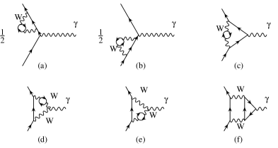
Figure 4: ${\cal O}(N_{f}\alpha^{2})$ photon vertex corrections.

Representative topologies for the ${\cal O}(N_{f}\alpha^{2})$ photon vertex diagrams contributing to Thomson scattering are shown in Fig.4. These may be calculated using methods described in ref.[25]. Diagrams of the type Fig.4e–f containing virtual photons or $Z^{0}$’s, instead of $W$ bosons, cancel by Ward identities and we have explicitly checked that this occurs. The sum of all diagrams in Fig.4 is

$$\equiv V_{i\gamma}^{(2)}(0)\gamma_{\mu}\gamma_{L}$$

$$= -ig\left(\frac{g^{2}}{16\pi^{2}}\right)^{2}8t_{3}s_{\theta}\gamma_{\mu}\gamma_{L}\frac{(\pi M_{W}^{2})^{n-4}}{n}\Gamma(4-n)\Gamma\left(2-\frac{n}{2}\right)\Gamma\left(\frac{n}{2}\right),$$

exactly for all $n$.

Figure 5: ${\cal O}(N_{f}\alpha^{2})$ corrections to the $Z$-$\gamma$ mixing, $\Pi^{(2)}_{Z\gamma}(0)$.

Representative diagrams contributing to $Z$-$\gamma$ mixing in ${\cal O}(N_{f}\alpha^{2})$ are shown in Fig.5. Again methods for calculating the individual diagrams may be found in ref.[25]. Upon summing all diagrams together one obtains the remarkably simple result

$$\equiv \delta_{\mu\nu}\Pi_{Z\gamma}^{(2b)}(0)$$

$$= \left(\frac{g^{2}}{16\pi^{2}}\right)^{2}8s_{\theta}c_{\theta}\delta_{\mu\nu}M_{Z}^{2}\frac{(\pi M_{W}^{2})^{n-4}}{n}\Gamma(4-n)\Gamma\left(2-\frac{n}{2}\right)\Gamma\left(\frac{n}{2}\right).$$

The ${\cal O}(N_{f}\alpha^{2})$ diagrams when added together must form a pure vector current proportional to the charge, $Q$, of the external fermion and independent of its weak isospin, $t_{3}$. Contributions from the photon self-energy, which will be dealt with later, are obviously of this form and cancellation of terms proportional to $t_{3}$ is expected between the vertex corrections, given above, and the $Z$-$\gamma$ mixing when it is coupled to the external fermion. This is indeed borne out and one obtains

$$V_{i\gamma}^{(2)}(0)\gamma_{\mu}\gamma_{L}+i\frac{g}{c_{\theta}}\gamma_{\mu}(t_{3}\gamma_{L}-s_{\theta}^{2}Q)\frac{\Pi_{Z\gamma}^{(2b)}(0)}{M_{Z}^{2}}=\\ -ig\left(\frac{g^{2}}{16\pi^{2}}\right)^{2}8Qs_{\theta}^{3}\gamma_{\mu}\frac{(\pi M_{W}^{2})^{n-4}}{n}\Gamma(4-n)\Gamma\left(2-\frac{n}{2}\right)\Gamma\left(\frac{n}{2}\right).$$ (67)

6.2.2 Counterterm Insertions

The ${\cal O}(N_{f}\alpha^{2})$ corrections coming from the insertion of 1-loop counterterms into 1-loop diagrams may be calculated using the expressions for the 2-point counterterms given in section 3 and simplified using the Ward identity (59). Note once again that contributions coming from the first term in the 2-point counterterm for the $W$ boson, (14), cancel against vertex counterterms. The result is

$$V_{i\gamma}^{(2\delta)}(0)\gamma_{\mu}\gamma_{L}=\frac{\delta g^{(1f)}}{g}ig\left(\frac{g^{2}}{16\pi^{2}}\right)3t_{3}s_{\theta}\gamma_{\mu}\gamma_{L}(\pi M_{W}^{2})^{-\epsilon}\Gamma(\epsilon)\\ -\frac{\delta M_{W}^{2(1f)}}{M_{W}^{2}}ig\left(\frac{g^{2}}{16\pi^{2}}\right)t_{3}s_{\theta}\gamma_{\mu}\gamma_{L}(\pi M_{W}^{2})^{-\epsilon}\epsilon\Gamma(\epsilon)$$ (68)

Similarly the ${\cal O}(N_{f}\alpha^{2})$ contribution from 1-loop counterterm insertions into the 1-loop $Z$-$\gamma$ mixing is

$$\Pi_{Z\gamma}^{(2\delta)}(0)=\frac{\delta g^{(1f)}}{g}\left(\frac{g^{2}s_{\theta}}{16\pi^{2}}\right)s_{\theta}c_{\theta}M_{Z}^{2}(\pi M_{W}^{2})^{-\epsilon}\Gamma(\epsilon)\\ -\delta M_{W}^{2(1f)}\left(\frac{g^{2}s_{\theta}}{16\pi^{2}}\right)\frac{s_{\theta}}{c_{\theta}}(\pi M_{W}^{2})^{-\epsilon}(2-\epsilon)\Gamma(\epsilon)$$ (69)

Individual self-energy diagrams contributing to eq.(46) contain pieces proportional to $g^{2}s_{\theta}c_{\theta}M_{W}^{2}$ and $g^{2}(s_{\theta}^{3}/c_{\theta})M_{W}^{2}$ and there is a very complex and intricate interplay between diagrams containing $W$ boson 2-point counterterms (14), scalar counterterms (39) the vector-scalar mixing counterterms (40) to produce an overall result proportional to $g^{2}(s_{\theta}/c_{\theta})M_{W}^{2}$. This, when connected to the external fermion by a $Z^{0}$ propagator leads to a result proportional simply to $g^{3}s_{\theta}$ of the same form as $V_{i\gamma}^{(2\delta)}(0)$ in eq.(68).

Combining eq.(68) and eq.(69) yields the total ${\cal O}(N_{f}\alpha^{2})$ contribution counterterm insertions in the vertex and $Z$-$\gamma$ mixing,

$$V_{i\gamma}^{(2\delta)}(0)\gamma_{\mu}\gamma_{L}+i\frac{g}{c_{\theta}}\gamma_{\mu}(t_{3}\gamma_{L}-s_{\theta}^{2}Q)\frac{\Pi_{Z\gamma}^{(2\delta)}(0)}{M_{Z}^{2}}=\\ \left(2\frac{\delta g^{(1f)}}{g}-\frac{\delta M_{W}^{2(1f)}}{M_{W}^{2}}\right)ig\left(\frac{g^{2}}{16\pi^{2}}\right)2t_{3}s_{\theta}\gamma_{\mu}\gamma_{L}(\pi M_{W}^{2})^{-\epsilon}\Gamma(\epsilon)\\ -\frac{\delta g^{(1f)}}{g}ig\left(\frac{g^{2}}{16\pi^{2}}\right)Qs_{\theta}^{3}\gamma_{\mu}(\pi M_{W}^{2})^{-\epsilon}\Gamma(\epsilon)\\ +\frac{\delta M_{W}^{2(1f)}}{M_{W}^{2}}ig\left(\frac{g^{2}}{16\pi^{2}}\right)Qs_{\theta}^{3}\gamma_{\mu}(\pi M_{W}^{2})^{-\epsilon}(2-\epsilon)\Gamma(\epsilon)$$ (70)

Note that the finite terms, proportional to $t_{3}\epsilon\Gamma(\epsilon)$ have canceled. The remaining part proportional to $t_{3}$ contributes to eq.(57) and therefore cancels with other terms as discussed in section 5. It will be discarded and only the second and third terms in eq.(70), proportional to $Q$, will be retained.

6.2.3 Counterterms

The expressions for the counterterms given in eq.(8), (9) and (36) are correct to ${\cal O}(\alpha^{2})$ and need to be specialized to ${\cal O}(N_{f}\alpha^{2})$. Using the Ward identities, (58) and (59), the $Z$-$\gamma$ mixing counterterm of eq.(9) becomes

$$= M_{Z}^{2}s_{\theta}c_{\theta}\bigg{\{}3\left(\frac{\delta g^{(1b)}}{g}.\frac{\delta g^{(1f)}}{g}-\frac{\delta g^{\prime(1b)}}{g^{\prime}}.\frac{\delta g^{\prime(1f)}}{g^{\prime}}\right)$$ (71)

$$\ \ \ \ \ \ \ \ \ \ \ \ \ -\frac{\delta M_{W}^{2(1f)}}{M_{W}^{2}}\left(\frac{1}{2}\delta Z_{W}^{(1b)}+\frac{\delta g^{(1b)}}{g}\right)\bigg{\}}$$

and the photon vertex counterterm, eq.(36), yields

$$= -igs_{\theta}t_{3}\gamma_{\mu}\gamma_{L}\bigg{\{}3\left(\frac{\delta g^{(1b)}}{g}.\frac{\delta g^{(1f)}}{g}-\frac{\delta g^{\prime(1b)}}{g^{\prime}}.\frac{\delta g^{\prime(1f)}}{g^{\prime}}\right)$$ (72)

$$\ \ \ \ \ \ \ \ \ \ \ \ \ \ \ \ \ \ \ \ -2\frac{\delta g^{(1f)}}{g}\left(\frac{1}{2}\delta Z_{W}^{(1b)}+\frac{\delta g^{(1b)}}{g}\right)\bigg{\}}$$

$$\ \ \ \ \ \ \ \ \ \ -igs_{\theta}Q\gamma_{\mu}3\frac{\delta g^{\prime(1b)}}{g^{\prime}}.\frac{\delta g^{\prime(1f)}}{g^{\prime}}$$

Their contribution to the Thomson scattering matrix element together is

$$\left(2\frac{\delta g^{(1f)}}{g}-\frac{\delta M_{W}^{2(1f)}}{M_{W}^{2}}\right)\left(\frac{1}{2}\delta Z_{W}^{(1b)}+\frac{\delta g^{(1b)}}{g}\right)ig2t_{3}s_{\theta}\gamma_{\mu}\gamma_{L}\\ +\frac{\delta M_{W}^{2(1f)}}{M_{W}^{2}}igQs_{\theta}^{3}\left(\frac{1}{2}\delta Z_{W}^{(1b)}+\frac{\delta g^{(1b)}}{g}\right)\gamma_{\mu}\\ -igs_{\theta}Q\,.\,3\left(s_{\theta}^{2}\frac{\delta g^{(1b)}}{g}.\frac{\delta g^{(1f)}}{g}+c_{\theta}^{2}\frac{\delta g^{\prime(1b)}}{g^{\prime}}.\frac{\delta g^{\prime(1f)}}{g^{\prime}}\right)\gamma_{\mu}$$ (73)

As discussed in section 5 the part proportional to $t_{3}$ can be shown to cancel against products of 1-loop counterterms coming from 1PR diagrams and will therefore be discarded.

It is convenient at this point to define a quantity, $\widehat{\Pi}_{Z\gamma}^{(2)}(0)$, obtained by combining the parts proportional to $Q$ of eq.(LABEL:eq:NfZgamma), eq.(70) and all but the last term in eq.(73). Hence

$$\widehat{\Pi}_{Z\gamma}^{(2)}(0) = \left(\frac{g^{2}}{16\pi^{2}}\right)^{2}8s_{\theta}c_{\theta}M_{Z}^{2}\frac{(\pi M_{W}^{2})^{n-4}}{n}\Gamma(4-n)\Gamma\left(2-\frac{n}{2}\right)\Gamma\left(\frac{n}{2}\right)$$ (74)

$$+\frac{\delta g^{(1f)}}{g}\left(\frac{g^{2}}{16\pi^{2}}\right)s_{\theta}c_{\theta}M_{Z}^{2}(\pi M_{W}^{2})^{-\epsilon}\Gamma(\epsilon)$$

$$-\frac{\delta M_{W}^{2(1f)}}{M_{W}^{2}}s_{\theta}c_{\theta}M_{Z}^{2}\left(\frac{1}{2}\delta Z_{W}^{(1b)}+\frac{\delta g^{(1b)}}{g}+2\left(\frac{g^{2}}{16\pi^{2}}\right)(\pi M_{W}^{2})^{-\epsilon}\Gamma(\epsilon)\right)$$

$$-\frac{\delta M_{W}^{2(1f)}}{M_{W}^{2}}\left(\frac{g^{2}}{16\pi^{2}}\right)s_{\theta}c_{\theta}M_{Z}^{2}(\pi M_{W}^{2})^{-\epsilon}(2-\epsilon)\Gamma(\epsilon).$$

Figure 6: ${\cal O}(N_{f}\alpha^{2})$ corrections to the photon self-energy, $\Pi^{\prime(2)}_{\gamma\gamma}(0)$.

6.3 The Photon Self-Energy

6.3.1 Diagrams

Representative topologies for the diagrams contributing to the photon self-energy, $\Pi_{\gamma\gamma}^{\prime}(0)$ of eq.(48) at ${\cal O}(N_{f}\alpha^{2})$ are shown in Fig.6. Calculation of the photon self-energy involves projecting out the transverse parts of individual diagrams followed by differentiation with respect to the external momentum squared using techniques described in ref.[25]. Individual diagrams are not separately transverse but we have checked that the longitudinal part vanishes when all diagrams are added together. The result is

$$\Pi_{\gamma\gamma}^{\prime(2)}(0) = \left(\frac{g^{2}s_{\theta}}{16\pi^{2}}\right)^{2}\frac{8}{3}\frac{(n+2)}{n}(\pi M_{W}^{2})^{n-4}\Gamma(4-n)\Gamma\left(2-\frac{n}{2}\right)\Gamma\left(\frac{n}{2}-1\right)$$

$$+ \left(\frac{g^{2}s_{\theta}}{16\pi^{2}}\right)^{2}\frac{4}{27c_{\theta}^{2}}(44s_{\theta}^{4}-27s_{\theta}^{2}+9)$$

$$\ \ \ \ \ \ \ \ \times\frac{(n-6)}{n}(\pi M_{Z}^{2})^{n-4}\Gamma(5-n)\Gamma\left(2-\frac{n}{2}\right)\Gamma\left(\frac{n}{2}-1\right)$$

$$- \left(\frac{g^{2}s_{\theta}}{16\pi^{2}}\right)^{2}\frac{4(n-2)}{3n}\pi^{n-4}(M_{W}^{2})^{\frac{n}{2}-2}\Gamma\left(3-\frac{n}{2}\right)\Gamma\left(2-\frac{n}{2}\right)\sum_{f}Q_{f}^{2}(m_{f}^{2})^{\frac{n}{2}-2}$$

$$- \left(\frac{g^{2}s_{\theta}}{16\pi^{2}}\right)^{2}\frac{8}{3}\pi^{n-4}(M_{W}^{2})^{\frac{n}{2}-2}\Gamma\left(2-\frac{n}{2}\right)^{2}\sum_{f}Q_{f}t_{3f}(m_{f}^{2})^{\frac{n}{2}-2}$$

$$- \left(\frac{g^{2}s_{\theta}}{16\pi^{2}}\right)^{2}\frac{16(n-2)}{3n}\pi^{n-4}(M_{Z}^{2})^{\frac{n}{2}-2}\Gamma\left(3-\frac{n}{2}\right)\Gamma\left(2-\frac{n}{2}\right)$$

$$\ \ \ \ \ \ \ \ \times\sum_{f}Q_{f}^{2}\left(\frac{\beta_{Lf}^{2}+\beta_{Rf}^{2}}{2}\right)(m_{f}^{2})^{\frac{n}{2}-2}$$

$$+ \left(\frac{g^{2}s_{\theta}}{16\pi^{2}}\right)^{2}\frac{16n}{3(n-2)}\pi^{n-4}(M_{Z}^{2})^{\frac{n}{2}-2}\Gamma\left(3-\frac{n}{2}\right)\Gamma\left(2-\frac{n}{2}\right)$$

$$\ \ \ \ \ \ \ \ \times\sum_{f}Q_{f}^{2}\beta_{Lf}\beta_{Rf}(m_{f}^{2})^{\frac{n}{2}-2}$$

$$+ \left(\frac{g^{2}s_{\theta}}{16\pi^{2}}\right)^{2}\frac{4s_{\theta}^{2}}{3}\frac{(5n^{2}-33n+34)}{n(n-5)}\pi^{n-4}\Gamma\left(3-\frac{n}{2}\right)\Gamma\left(2-\frac{n}{2}\right)\sum_{f}Q_{f}^{4}(m_{f}^{2})^{n-4}$$

Contributions that are suppressed by factors $m_{f}^{2}/M_{W}^{2}$ relative to the leading terms have been dropped. The first term on the right hand side of eq.(LABEL:eq:twoloopphotonse) comes from diagrams Fig.6a–e that contain an internal $W$ boson, the second comes from diagrams Fig.6f&g containing an internal $Z^{0}$. The last term in eq.(LABEL:eq:twoloopphotonse) comes from diagrams Fig.6h&i that are pure QED in nature. Contributions for which the fermion mass can be safely set to zero without affecting the final result were be obtained using the methods described in ref.[25]. The terms in which the fermion mass appears are obtained using the asymptotic expansion of ref.[26]. It should be noted that setting $m_{f}=0$ in Fig.6c–g does not immediately cause obvious problems in the computation because the diagram still contains one non-vanishing scale. A certain amount of care is thus required to identify situations in which the fermion mass cannot be discarded. In the case of the photon self-energy, the need to include such terms is indicated by divergences proportional to the $\ln m_{f}^{2}$ in the counterterm insertion diagrams. All diagrams that yield $m_{f}$-dependent terms can be split in two by a cut through two internal fermion propagators. The contributions are therefore precisely those that are accessed via dispersion relations (54).

As it stands the eq.(LABEL:eq:twoloopphotonse) for $\Pi_{\gamma\gamma}^{\prime(2)}(0)$ contains a divergence, in its fourth term, with a coefficient that depends on $\ln m_{f}^{2}$. It will be seen in the next section that this is canceled by a counterterm insertion. There remain finite terms depending on the fermion mass that must be treated using dispersion relations when the internal fermions are quarks.

6.3.2 Counterterm Insertions

The ${\cal O}(N_{f}\alpha^{2})$ corrections coming from 1-loop counterterm insertions into 1-loop diagrams for the transverse part of the photon self-energy may be calculated to be

$$\Pi_{\gamma\gamma}^{\prime(2\delta)}(0) = 2\frac{\delta g^{(1f)}}{g}\left(\frac{g^{2}s_{\theta}^{2}}{16\pi^{2}}\right)(\pi M_{W}^{2})^{-\epsilon}\Gamma(\epsilon)$$ (76)

$$+\frac{\delta M_{W}^{2(1f)}}{M_{W}^{2}}\left(\frac{g^{2}s_{\theta}^{2}}{16\pi^{2}}\right)\left(\frac{2}{3}\epsilon-5\right)(\pi M_{W}^{2})^{-\epsilon}\epsilon\Gamma(\epsilon)$$

$$-\left(\frac{\delta g^{(1b)}}{g}+\frac{1}{2}\delta Z_{W}^{(1b)}\right)\left(\frac{g^{2}s_{\theta}^{2}}{16\pi^{2}}\right)\frac{4}{3}\pi^{-\epsilon}\Gamma(\epsilon)\sum_{f}Q_{f}t_{3f}(m_{f}^{2})^{-\epsilon}$$

$$+\left(\frac{g^{2}s_{\theta}^{2}}{16\pi^{2}}\right)\frac{8}{3}\pi^{-\epsilon}\epsilon\Gamma(\epsilon)\sum_{f}Q_{f}^{2}\frac{\delta m_{f}^{(1b)}}{m_{f}}(m_{f})^{-\epsilon}$$

It was checked that the longitudinal form factor vanishes which involves, once again, an intricate interplay between diagrams containing $W$-boson 2-point counterterms (14), scalar counterterms (39) and vector-scalar mixing counterterms (40).

By virtue of (60), the second term on the right-hand side of eq.(76) cancels the divergence in the fourth term of eq.(LABEL:eq:twoloopphotonse) that depends on $\ln m_{f}^{2}$. It may also be seen by substituting the expression for $\delta m_{f}$ in eq.(34) into eq.(76) that the remaining terms that depend on $m_{f}$ in $\Pi_{\gamma\gamma}^{\prime(2)}(0)$ are rendered finite by the counterterm insertions with the exception of the last. Moreover, in the on-shell renormalization scheme, there is an exact cancellation and these finite terms are eliminated completely. At 1-loop the bosonic and fermionic sectors of the theory are renormalized independently of one another. It is obviously a great convenience and simplification here to demand that the internal fermions are renormalized in the on-shell scheme. This will be done in the following but no such constraint will be imposed on the bosonic sector.

Combining eq.(LABEL:eq:twoloopphotonse) and eq.(76) we define a new quantity, $\widehat{\Pi}_{\gamma\gamma}^{\prime(2)}(0)=\Pi_{\gamma\gamma}^{\prime(2)}(0)+\Pi_{\gamma\gamma}^{\prime(2\delta)}(0)$, given by

$$\widehat{\Pi}_{\gamma\gamma}^{\prime(2)}(0) = \left(\frac{g^{2}s_{\theta}}{16\pi^{2}}\right)^{2}\frac{8}{3}\frac{(n+2)}{n}(\pi M_{W}^{2})^{n-4}\Gamma(4-n)\Gamma\left(2-\frac{n}{2}\right)\Gamma\left(\frac{n}{2}-1\right)$$ (77)

$$+ \left(\frac{g^{2}s_{\theta}}{16\pi^{2}}\right)^{2}\frac{4}{27c_{\theta}^{2}}(44s_{\theta}^{4}-27s_{\theta}^{2}+9)$$

$$\ \ \ \ \ \ \ \ \times\frac{(n-6)}{n}(\pi M_{Z}^{2})^{n-4}\Gamma(5-n)\Gamma\left(2-\frac{n}{2}\right)\Gamma\left(\frac{n}{2}-1\right)$$

$$+ 2\left(\frac{g^{2}s_{\theta}^{2}}{16\pi^{2}}\right)\frac{\delta g^{(1f)}}{g}(\pi M_{W}^{2})^{\frac{n}{2}-2}\Gamma\left(2-\frac{n}{2}\right)$$

$$- \left(\frac{g^{2}s_{\theta}^{2}}{16\pi^{2}}\right)\frac{\delta M_{W}^{2(1f)}}{M_{W}^{2}}\left(\frac{n+11}{3}\right)(\pi M_{W}^{2})^{\frac{n}{2}-2}\Gamma\left(3-\frac{n}{2}\right)$$

$$- \left(\frac{g^{2}s_{\theta}^{2}}{16\pi^{2}}\right)\frac{4}{3}\left(\frac{\delta g^{(1b)}}{g}+\frac{1}{2}\delta Z_{W}^{(1b)}+2\left(\frac{g^{2}}{16\pi^{2}}\right)(\pi M_{W}^{2})^{\frac{n}{2}-2}\Gamma\left(2-\frac{n}{2}\right)\right)$$

$$\ \ \ \ \ \ \ \ \times\pi^{\frac{n}{2}-2}\Gamma\left(2-\frac{n}{2}\right)\sum_{f}Q_{f}t_{3f}(m_{f}^{2})^{\frac{n}{2}-2}$$

$$+ \left(\frac{g^{2}s_{\theta}^{2}}{16\pi^{2}}\right)^{2}\frac{4(n^{3}-12n^{2}+41n-34)}{n(n-3)(n-5)}\pi^{n-4}\Gamma\left(3-\frac{n}{2}\right)\Gamma\left(2-\frac{n}{2}\right)$$

$$\ \ \ \ \ \ \ \ \times\sum_{f}Q_{f}^{4}(m_{f}^{2})^{n-4}$$

Of the two remaining terms in eq.(77) that depend on $m_{f}$, the first corresponds to weak corrections to photon-fermion vertex that have their origin in the diagram of Fig.6e. The second comes from the pure QED diagrams, Fig.6h&i, and their associated fermion mass counterterms. When expanded about $n=4$ its leading logarithms reproduce the well-known result of Jost and Luttinger [27]. Both sets can be treated via the dispersion relation trick, eq.(52). This requires that the diagrams be evaluated at some high $\hat{q}^{2}$. Fig.6e at high $\hat{q}^{2}$ contains two unrelated scales and cannot be treated by the techniques used so far. In principle it can be obtained in closed analytic form from results given by Scharf and Tausk [28] but it is neither compact nor illuminating and probably best obtained numerically.

The pure QED diagrams of Fig.6h&i are exactly calculable for $|\hat{q}^{2}|\gg m_{f}^{2}$. The result is

$$\Pi_{\gamma\gamma}^{\prime(2{\rm QED})}(\hat{q}^{2})=-\sum_{f}\left(\frac{g^{2}}{16\pi^{2}}\right)^{2}Q_{f}^{4}s_{\theta}^{4}(\pi\hat{q}^{2})^{n-4}\\ \times\Bigg{\{}8(n^{2}-7n+16)\frac{\Gamma\left(2-\frac{\displaystyle n}{\displaystyle 2}\right)^{2}\Gamma\left(\frac{\displaystyle n}{\displaystyle 2}\right)^{3}\Gamma\left(\frac{\displaystyle n}{\displaystyle 2}-2\right)}{\Gamma(n)\Gamma(n-1)}\\ +24\frac{(n^{2}-4n+8)}{(n-1)(n-4)}.\frac{\Gamma(4-n)\Gamma\left(\frac{\displaystyle n}{\displaystyle 2}\right)^{2}\Gamma\left(\frac{\displaystyle n}{\displaystyle 2}-2\right)}{\Gamma\left(\frac{\displaystyle 3n}{\displaystyle 2}-2\right)}\Bigg{\}}$$ (78)

Broadhurst et al. [29] have given an expression for the subtracted photon vacuum polarization at general $q^{2}$. The high-energy limit can be obtained by applying analytic continuation relations for the hypergeometric functions, ${}_{2}F_{1}$ and ${}_{3}F_{2}$ that appear in their result.

Despite appearances, the expression on the right hand side of eq.(78) has only a simple pole with a constant coefficient at $n=4$ that can be canceled by local counterterms. The leading logarithmic expressions can be found in ref.[30, section 8-4-4] where the authors invite the “foolhardy reader” to check that the finite parts are transverse. Here we have gone further and demonstrated this property in the exact result.

It can be checked that the divergent part of (78) is identical to that of the last term in eq.(77) so that that the difference $\mathop{\rm Re}\nolimits\Pi_{\gamma\gamma}^{\prime(f)}(\hat{q}^{2})-\Pi_{\gamma\gamma}^{\prime(f)}(0)$ is finite. This provides yet another useful check of various aspects of the calculation.

6.4 Charge renormalization in a general scheme

All the ingredients are now in place to write down the complete set of ${\cal O}(N_{f}\alpha^{2})$ corrections to the Thomson scattering matrix element and from it obtain an expression, extending eq.(55), for the physical electromagnetic charge of a fermion in terms of the renormalized parameters of the theory.

Gathering all the parts together gives our main result

$$\sqrt{4\pi\alpha}=e\bigg{\{}1 +\frac{1}{2}\Pi_{\gamma\gamma}^{\prime(1)}(0)-\frac{s_{\theta}}{c_{\theta}}\frac{\Pi_{Z\gamma}^{(1b)}(0)}{M_{Z}^{2}}+s_{\theta}^{2}\frac{\delta g^{(1)}}{g}+c_{\theta}^{2}\frac{\delta g^{\prime(1)}}{g^{\prime}}$$

$$+\frac{1}{2}\widehat{\Pi}_{\gamma\gamma}^{\prime(2)}(0)-\frac{s_{\theta}}{c_{\theta}}\frac{\widehat{\Pi}_{Z\gamma}^{(2)}(0)}{M_{Z}^{2}}+\Pi^{{\rm 1PR}}(0)+s_{\theta}^{2}\frac{\delta g^{(2)}}{g}+c_{\theta}^{2}\frac{\delta g^{\prime(2)}}{g^{\prime}}$$

$$-3\left(s_{\theta}^{2}\frac{\delta g^{(1b)}}{g}.\frac{\delta g^{(1f)}}{g}+c_{\theta}^{2}\frac{\delta g^{\prime(1b)}}{g^{\prime}}.\frac{\delta g^{\prime(1f)}}{g^{\prime}}\right)\bigg{\}}$$ (79)

where $\widehat{\Pi}_{\gamma\gamma}^{\prime(2)}(0)$ is given in eq.(77), $\widehat{\Pi}_{Z\gamma}^{(2)}(0)$ in eq.(74) and $\Pi^{{\rm 1PR}}(0)$ in eq.(63).

7 ${\cal O}(N_{f}\alpha^{2})$ wavefunction counterterms

Up to this point we have been pursuing the expression for the physical matrix element for Thomson scattering and, to that end, terms that do not contribute to the final result have often been discarded. Although the final result does not depend on the ${\cal O}(N_{f}\alpha^{2})$ wavefunction renormalization counterterms, $\delta Z_{W}^{(2)}$ and $\delta Z_{B}^{(2)}$, the Green’s functions that have been calculated in the foregoing allow relations to be determined between them and $\delta g^{(2)}$ and $\delta g^{\prime(2)}$. In all cases the leading divergences of these counterterms, i.e. those corresponding to a double pole at $n=4$, are independent of renormalization scheme but subleading and finite parts will depend on which renormalization scheme has been chosen.

When the ${\cal O}(N_{f}\alpha^{2})$ diagrams contributing to $Z$-$\gamma$ mixing (LABEL:eq:NfZgamma) are combined with the counterterm insertions (69) and the counterterms (9) the result must be finite in any scheme. One thus obtains

$$\left(\frac{g^{2}}{16\pi^{2}}\right)^{2}8\frac{(\pi M_{W}^{2})^{n-4}}{n}\Gamma(4-n)\Gamma\left(2-\frac{n}{2}\right)\Gamma\left(\frac{n}{2}\right)+\frac{\delta g^{(1f)}}{g}\left(\frac{g^{2}}{16\pi^{2}}\right)(\pi M_{W}^{2})^{-\epsilon}\Gamma(\epsilon)$$

$$+\frac{\delta M_{W}^{2(1f)}}{M_{W}^{2}}\left(\frac{g^{2}}{16\pi^{2}}\right)(\pi M_{W}^{2})^{-\epsilon}\epsilon\Gamma(\epsilon)$$

$$-\frac{\delta M_{W}^{2(1f)}}{M_{W}^{2}}\left(\frac{1}{2}\delta Z_{W}^{(1b)}+\frac{\delta g^{(1b)}}{g}+2\left(\frac{g^{2}}{16\pi^{2}}\right)(\pi M_{W}^{2})^{-\epsilon}\Gamma(\epsilon)\right)$$ (80)

$$+3\left(\frac{\delta g^{(1b)}}{g}.\frac{\delta g^{(1f)}}{g}-\frac{\delta g^{\prime(1b)}}{g^{\prime}}.\frac{\delta g^{\prime(1f)}}{g^{\prime}}\right)-\frac{\delta g^{(2)}}{g}+\frac{\delta g^{\prime(2)}}{g^{\prime}}-\frac{1}{2}\delta Z_{W}^{(2)}+\frac{1}{2}\delta Z_{B}^{(2)}=\mbox{finite}$$

Turning to the ${\cal O}(N_{f}\alpha^{2})$ corrections to the photon vertex it similarly follows that when the contributions from diagrams, (LABEL:eq:Nfalphavertex), counterterm insertions, (68), and pure counterterms (36) are added together the result is finite. The part of the vertex proportional to $t_{3}$ yields the condition

$$\left(\frac{g^{2}}{16\pi^{2}}\right)^{2}8\frac{(\pi M_{W}^{2})^{n-4}}{n}\Gamma(4-n)\Gamma\left(2-\frac{n}{2}\right)\Gamma\left(\frac{n}{2}\right)+\frac{\delta g^{(1f)}}{g}\left(\frac{g^{2}}{16\pi^{2}}\right)(\pi M_{W}^{2})^{-\epsilon}\Gamma(\epsilon)$$

$$+\frac{\delta M_{W}^{2(1f)}}{M_{W}^{2}}\left(\frac{g^{2}}{16\pi^{2}}\right)(\pi M_{W}^{2})^{-\epsilon}\epsilon\Gamma(\epsilon)$$

$$-2\frac{\delta g^{(1f)}}{g}\left(\frac{1}{2}\delta Z_{W}^{(1b)}+\frac{\delta g^{(1b)}}{g}+2\left(\frac{g^{2}}{16\pi^{2}}\right)(\pi M_{W}^{2})^{-\epsilon}\Gamma(\epsilon)\right)$$ (81)

$$+3\left(\frac{\delta g^{(1b)}}{g}.\frac{\delta g^{(1f)}}{g}-\frac{\delta g^{\prime(1b)}}{g^{\prime}}.\frac{\delta g^{\prime(1f)}}{g^{\prime}}\right)-\frac{\delta g^{(2)}}{g}+\frac{\delta g^{\prime(2)}}{g^{\prime}}-\frac{1}{2}\delta Z_{W}^{(2)}+\frac{1}{2}\delta Z_{B}^{(2)}=\mbox{finite}$$

This expression differs from the previous one but is consistent with it because of the finiteness of the combinations (60) and (61). This consistency is a stringent check of very many aspects of the calculation.

The part of the the photon vertex proportional to $Q$ leads to the condition

$$\frac{\delta g^{\prime(2)}}{g^{\prime}}+\frac{1}{2}\delta Z_{B}^{(2)}-3\left(\frac{\delta g^{\prime(1b)}}{g^{\prime}}.\frac{\delta g^{\prime(1f)}}{g^{\prime}}\right)=\mbox{finite}.$$ (82)

Obviously eq.s(81) and (82) can be used to obtain a condition for the combination of counterterms

$$\frac{\delta g^{(2)}}{g}+\frac{1}{2}\delta Z_{W}^{(2)}+2\frac{\delta g^{(1f)}}{g}\left(\frac{1}{2}\delta Z_{W}^{(1b)}+\frac{\delta g^{(1b)}}{g}\right)-3\frac{\delta g^{(1b)}}{g}.\frac{\delta g^{(1f)}}{g}$$

which is the ${\cal O}(N_{f}\alpha^{2})$ $W$-fermion coupling counterterm and occurs, for example, in the calculation of corrections to the muon lifetime. Indeed this fact has been exploited as an extremely stringent cross check of both the results of this paper and of the calculation ${\cal O}(N_{f}\alpha^{2})$ corrections to the muon lifetime [31].

The corrections to photon self-energy calculated in section 6.3 yield an independent condition on the the ${\cal O}(N_{f}\alpha^{2})$ counterterms

$$s_{\theta}^{2}\delta Z_{W}^{(2)}+c_{\theta}^{2}\delta Z_{B}^{(2)}+\widehat{\Pi}_{\gamma\gamma}^{\prime(2)}(0)=\mbox{finite}$$ (83)

where $\widehat{\Pi}_{\gamma\gamma}^{\prime(2)}(0)$ is given in eq.(77).

8 Summary

The complete ${\cal O}(N_{f}\alpha^{2})$ renormalization of the electromagnetic charge in the Standard Model using a general renormalization scheme has been presented. This represents the first practical calculation in which the full structure of the 2-loop renormalization has been confronted and lays the groundwork for future calculations of this type. The results have already been exploited in the calculation of the ${\cal O}(N_{f}\alpha^{2})$ corrections to the muon lifetime.

The $Z$-$\gamma$ mixing adds considerably to the overall complexity and number of Feynman diagrams that must be considered. Contributions coming from the insertion of 1-loop counterterms in 1-loop diagrams constitute a significant portion of the calculation due partly to the appearance at this order of counterterms that mix vector bosons with scalars.

All integrals were performed exactly in dimensional regularization without expanding in $\epsilon=2-n/2$ yet in many cases they produced new and remarkably simple expressions that display the full analytic structure of the results.

The rôle of wavefunction counterterms was investigated. It was found that the ${\cal O}(\alpha)$ wavefunction counterterms, $\delta Z^{(1)}$, had to be included in a manner consistent with Ward identities but that the ${\cal O}(N_{f}\alpha^{2})$ counterterms, $\delta Z^{(2)}$, could be neglected since they cancel in the final physical result. The price for this is that one must deal with divergent Greens functions in intermediate steps.

A large number of internal consistency checks were performed in the course of the calculation in order to ensure the correctness of the results presented here.

References

- [1] A. D. Martin and D. Zeppenfeld, Phys. Lett. B 345 (1995) 558.
- [2] S. Eidelman and F. Jegerlehner, Z. Phys. C 76 (1995) 585.
- [3] M. L. Swartz, Phys. Rev. D 53 (1996) 5268.
- [4] M. Davier and A. Höcker, hep-ph/9711308.
- [5] J. H. Kühn and M. Steinhauser, hep-ph/9802241.
- [6] R. G. Stuart Phys. Rev. D 52 (1995) 1655.
- [7] R. Barbieri et al., Phys. Lett. B 288 (1992) 95; errata ibid B 312 (1993) 511.
- [8] R. Barbieri et al., Nucl. Phys. B 409 (1993) 105.
- [9] J. Fleischer, O. V. Tarasov and F. Jegerlehner, Phys. Lett. B 319 (1993) 249.
- [10] J. Fleischer, O. V. Tarasov and F. Jegerlehner, Phys. Rev. D 51 (1995) 3820.
- [11] G. Degrassi, P. Gambino and A. Vicini, Phys. Lett. B 383 (1996) 219.
- [12] A. Czarnecki, B. Krause and W. J. Marciano, Phys. Rev. D 52 (1995) 2619.
- [13] A. Czarnecki, B. Krause and W. J. Marciano, Phys. Rev. Lett. 76 (1996) 3267.
- [14] D. A. Ross and J. C. Taylor, Nucl. Phys. B 51 (1973) 125.
- [15] K. I. Aoki et al, or, Suppl. Progr. Theor. Phys. 73 (1982) 1.
- [16] L. Baulieu and R. Coquereaux, Ann. Phys. 140 (1982) 163.
- [17] R. G. Stuart, D. Phil. thesis, University of Oxford; Rutherford-Appleton Laboratory Report RAL-T008, (1985)
- [18] M. Böhm, W. Hollik and H. Spiesberger, Fortschr. Phys. 34 (1986) 687.
- [19] A. Sirlin, Phys. Rev. D 22 (1980) 971.
- [20] W. F. L. Hollik, Fortschr. Phys. 38 (1990) 165.
- [21] A. Sirlin, Phys. Lett. B 232 (1990) 537.
- [22] R. G. Stuart, Phys. Lett. B 272 (1991) 353.
- [23] R. G. Stuart, Phys. Rev. Lett. 70 (1993) 3193.
- [24] W. J. Marciano and A. Sirlin, Phys. Rev. D 22 (1980) 2695; (E) D 31 (1985) 231.
- [25] R. Akhoury, P. Malde and R. G. Stuart, hep-ph/9707520.
- [26] A. I. Davydychev and J. B. Tausk, Nucl. Phys. B 397 (1993) 123.
- [27] R. Jost and J. M. Luttinger, Helv. Phys. Acta 23 (1950) 201.
- [28] R. Scharf and J. B. Tausk, Nucl. Phys. B 412 (1994) 523.
- [29] D. J. Broadhurst, J. Fleischer and O. V. Tarasov, Z. Phys. C 60 (1993) 287.
- [30] C. Itzykson and J.-B. Zuber, Quantum Field Theory, McGraw-Hill (1980).
- [31] P. Malde and R. G. Stuart, in preparation.