Abstract

Applications of perturbative QCD to deeply virtual Compton scattering and hard exclusive meson electroproduction processes require a generalization of usual parton distributions for the case when long-distance information is accumulated in nonforward matrix elements $\langle p^{\prime}\,|\,{\cal O}(0,z)\,|\,p\rangle$ of quark and gluon light-cone operators. In our previous papers we used two types of nonperturbative functions parametrizing such matrix elements: double distributions $F(x,y;t)$ and nonforward distribution functions ${\cal F}_{\zeta}(X;t)$. Here we discuss in more detail the double distributions (DDs) and evolution equations which they satisfy. We propose simple models for $F(x,y;t=0)$ DDs with correct spectral and symmetry properties which also satisfy the reduction relations connecting them to the usual parton densities $f(x)$. In this way, we obtain self-consistent models for the $\zeta$-dependence of nonforward distributions. We show that, for small $\zeta$, one can easily obtain nonforward distributions (in the $X>\zeta$ region) from the parton densities: ${\cal F}_{\zeta}(X;t=0)\approx f(X-\zeta/2)$.

PACS number(s): 12.38.Bx, 13.60.Fz, 13.60.Le

I Introduction

Applications of perturbative QCD to deeply virtual Compton scattering and hard exclusive electroproduction processes [1, 2, 3, 4, 5, 6, 7] require a generalization of usual parton distributions for the case when long-distance information is accumulated in nonforward matrix elements $\langle p-r\,|\,{\cal O}(0,z)\,|\,p\rangle\,|\,_{z^{2}=0}$ of quark and gluon light-cone operators. As argued in Refs. [2, 4, 5], such matrix elements can be parametrized by two basic types of nonperturbative functions. With $z$ taken in the lightcone “minus” direction, the double distributions (DDs) $F(x,y;t)$ specify the light-cone “plus” fractions $xp^{+}$ and $yr^{+}$ of the initial hadron momentum $p$ and the momentum transfer $r$ carried by the initial parton. Though $z$ is an integration variable, only one direction on the lightcone (specified by external momenta) is important for the lightcone-dominated processes. In other words, only the lightcone plus direction of the hadron $p$ and $r$ momenta are essential for such processes. By definition, the DDs $F(x,y;t)$ do not depend on the $r^{+}/p^{+}$ ratio. On the other hand, treating the proportionality coefficient as an independent parameter: $r^{+}\equiv\zeta p^{+}$, one can introduce an alternative description in terms of the nonforward parton distributions ${\cal F}_{\zeta}(X;t)$ with $X=x+y\zeta$ being the total fraction of the initial hadron momentum taken by the initial parton. The shape of the functions ${\cal F}_{\zeta}(X;t)$ explicitly depends on the parameter $\zeta$ characterizing the skewedness of the relevant nonforward matrix element. This parametrization of nonforward matrix elements by ${\cal F}_{\zeta}(X;t)$ is similar to that proposed originally by X. Ji [1, 3] who introduced off-forward parton distributions (OFPDs) $H(x,\xi;t)$. The latter are close to functions considered earlier in Ref. [8]. The functions $H(x,\xi;t)$ have a simple relation to nonforward distributions (NFPDs) ${\cal F}_{\zeta}(X;t)$, while the non-diagonal distributions $F(x_{1},x_{2})$ discussed by Collins, Frankfurt and Strikman [7] essentially coincide with ${\cal F}_{\zeta=x_{1}-x_{2}}(x_{1};t=0)$ (see Ref. [5] for details). The basic distinction between our approach and those of Refs. [1, 3, 7] is that we treat the double distributions $F(x,y;t)$ as the primary objects of the QCD analysis producing the nonforward distributions ${\cal F}_{\zeta}(X;t)$ (and other types of distributions) after an appropriate integration.

The formalism of double distributions provides a rather effective tool for studying some general (e.g., spectral) properties of NFPDs and it allows to find analytic solutions of evolution equations [2, 4, 5]. Incorporating symmetries of DDs [9] imposes rather strong restrictions on realistic models of NFPDs. A possible strategy for a self-consistent model building is to use nonperturbative or phenomenological approaches (MIT bag, quark models, QCD sum rule ideas, etc.) to construct double distributions at low normalization point and then evolve them to higher $Q^{2}$ values.

The evolution equation for the nonsinglet quark double distribution was derived in Ref.[2], where its analytic solution was also given. Evolution of the gluon distribution in pure gluodynamics was discussed in Refs.[4, 5]. In this paper, we present also a full set of evolution equations for the flavor-singlet case and derive a solution following the method of Refs.[2, 4, 5]. An independent study of singlet evolution based on our approach was performed in Ref.[10]. Evolution equations for various versions of nonforward distributions can be found in [3, 5, 11, 12, 13]. A convenient way to obtain the relevant evolution kernels is to use the universal light-ray evolution kernels [12, 13, 14, 15]. The evolution of nonforward distributions was studied numerically in refs.[11, 16, 9, 17, 18].

In the present paper, we incorporate the spectral and symmetry properties of double distributions to construct some simple models for DDs. Using the relations between DDs and NFPDs/OFPDs, we derive models for the latter and show that using the formalism of double distributions we can easily explain characteristic qualitative and quantitative features of the evolution of nonforward distributions observed in Refs.[11, 17].

II Basic definitions

The kinematics of the amplitudes of the DVCS process $\gamma^{*}(q)N(p)\to\gamma(q^{\prime})N(p^{\prime})$ and hard electroproduction $\gamma^{*}(q)N(p)\to M(q^{\prime})N(p^{\prime})$ can be specified by the initial nucleon momentum $p$, the momentum transfer $r=p-p^{\prime}$ and the momentum $q^{\prime}$ of the final photon or meson. To get a Bjorken-type scaling limit, one should also keep the invariant momentum transfer $t\equiv r^{2}$ small compared to the virtuality $-Q^{2}\equiv(q-r)^{2}$ of the initial photon and the energy invariant $p\cdot q\equiv m_{p}\nu$. The essential features of the hard electroproduction processes (DVCS included) can be most easily demonstrated if we set $q^{\prime 2}=0$, $p^{2}=0$, $r^{2}=0$ and use $p$, $q^{\prime}$ as the basic light-cone (Sudakov) 4-vectors. It is easy to see that the requirement $p^{\prime 2}\equiv(p+r)^{2}=p^{2}$ reduces in this limit to the condition $p\cdot r=0$ which can be satisfied only if the two lightlike momenta $p$ and $r$ are proportional to each other: $r=\zeta p$, where $\zeta$ coincides with the Bjorken variable $\zeta=x_{Bj}\equiv Q^{2}/2(p\cdot q)$. The latter satisfies the constraint $0\leq x_{Bj}\leq 1$. For small but finite $t$ and $m_{p}$, the momentum transfer $r$ still must have a non-zero plus component $r^{+}=\zeta p^{+}$. It also may have a transverse component $r_{\perp}$.

In the pQCD factorization treatment of hard electroproduction processes, the nonperturbative information is accumulated in the nonforward matrix element $\langle p-r\,|\,\varphi(0)\varphi(z)\,|\,p\rangle$ (we use here $\varphi$ as a generic notation for quark ($\psi$) or gluonic ($G$) fields). It depends on the relative coordinate $z$ through three invariant variables $(pz),(rz)$ and $z^{2}$. In the forward case, when $r=0$, one gets the usual parton distributions by Fourier transforming the light-cone projected (i.e., $z^{2}=0$) matrix element with respect to $(pz)$. In the nonforward case, we can try to start with the general Fourier representation

$$\langle p-r\,|\,\varphi(0)\varphi(z)\,|\,p\rangle\equiv{\cal M}((pz),(rz),z^{2};t,m_{p}^{2})=\int_{-\infty}^{\infty}dx\,\int_{-\infty}^{\infty}dy\,\int_{-\infty}^{\infty}e^{-ix(pz)-iy(rz)}\rho(x,y,\nu;t)\,e^{-iz^{2}\nu}d\nu$$ (1)

with respect to all three $z$-dependent invariants. The Fourier transform $\rho(x,y,\nu;t)$ can be called a triple distribution. Note that the generous $({-\infty},{\infty})$ limits for all three variables $x,y,\nu$ serve for a most general function of $(zp),(zr)$ and $z^{2}$. However, incorporating information that the Fourier transformation is written for a function ${\cal M}$ given by Feynman integrals having specific causality properties, one arrives at more narrow limits: $\nu$ runs from 0 to $\infty$, $x$ is between $-1$ and 1 while $y$ is between $0$ and 1 (this was proven in [5] for any Feynman diagram using the approach of Ref. [19]). To interpret the $x$-variable as the fraction of the initial momentum $p$ carried by the relevant parton, it makes sense to separate integration over positive and negative $x$ components and redefine $x\to-x$ and $y\to 1-y$ for the negative $x$ component. After that, the $x$-variable is always positive and $x$ and $y$ are further constrained by inequality $0\leq x+y\leq 1$ [2, 5]. These spectral conditions can be summarized by the following representation

$$\langle p-r\,|\,\varphi(0)\varphi(z)\,|\,p\rangle=$$ (2)

$$\hskip 42.67912pt\int_{0}^{\infty}d\nu\,e^{-i\nu(z^{2}-i\epsilon)}\int_{0}^{1}\int_{0}^{1}\biggl{[}e^{-ix(pz)-iy(rz)}\Phi(x,y,\nu;t)+e^{ix(pz)-i(1-y)(rz)}\bar{\Phi}(x,y,\nu;t)\biggl{]}\theta(x+y\leq 1)\,dx\,dy\,,$$ (3)

in which $\Phi(x,y,\nu;t)$ and $\bar{\Phi}(x,y,\nu;t)$ result from positive-$x$ and negative-$x$ components of $\rho(x,y,\nu;t)$ respectively. In particular, for quark operators, $\Phi(x,y,\nu;t)$ can be interpreted as the quark distribution while $\bar{\Phi}(x,y,\nu;t)$ as the antiquark one (a more detailed discussion is given in the next section). Similarly, $y$ and $(1-y)$ can be interpreted as the fractions in which the momentum transfer $r$ is shared among the two fields of the composite operator $\varphi(0)\varphi(z)$. Finally, the $\nu$ variable characterizes the virtuality of these fields. For a light-cone dominated process, the leading term is given by the $z^{2}\to 0$ limit of the nonforward matrix element, i.e. by zeroth moment of $\Phi(x,y,\nu;t)$ with respect to $\nu$

$$F(x,y;t)=\int_{0}^{\infty}\Phi(x,y,\nu;t)\,d\nu\,,$$ (4)

where $F(x,y;t)$ is the double distribution.

For a lightlike interval $z^{2}=0$, one can treat $z$ as having only light-cone “minus” component, and then the scalar products $(pz),(rz)$ project out the “plus” components of general (non-lightlike) momenta $p$ and $r$. This allows to give a parton interpretation of $F(x,y;t)$ as a probability amplitude for the active parton to carry fractions $xp^{+}$ and $yr^{+}$ of the plus components of the external momenta $r$ and $p$. Though the momenta $p^{+}$ and $r^{+}$ can be treated as proportional to each other $r^{+}=\zeta p^{+}$, $p^{+}$ and $r^{+}$ specify the “+”-momentum flow in two different channels. For $r^{+}=0$, the net “+”-momentum flows only in the $s$-channel and the total “+”-momentum entering into the composite operator vertex is zero. In this case, the matrix element is analogous to a distribution function. The partons entering the composite vertex then carry the fractions $x_{i}p^{+}$ of the initial proton momentum ($-1<x_{i}<1$). When $x_{i}$ is negative, we interpret the parton as belonging to the final state to secure that the integral always runs over the segment $0\leq x\leq 1$. In this parton picture, the spectators take the remaining momentum $(1-x)p^{+}$. On the other hand, if the total “+”-momentum flowing through the composite vertex is $r^{+}$, the matrix element has the structure of a distribution amplitude in which the momentum $r^{+}$ splits into the fractions $yr^{+}$ and $(1-y)r^{+}\equiv\bar{y}r^{+}$ carried by the two fields that appear in the vertex. In a combined situation, when both $p^{+}$ and $r^{+}$ are nonzero, the initial parton takes $xp^{+}+yr^{+}$, while the final one carries the momentum $xp^{+}-\bar{y}r^{+}$. For $r=0$, we get the forward matrix element which is parametrized by the usual parton distributions $f(x)$. This gives reduction relations [2, 4, 5] connecting double distributions with the usual ones (see Eqs.(12),(13) below).

III Quark and gluon distributions

For quark operators, the double distributions are defined by the following representation [2]:

$$\langle p^{\prime},s^{\prime}\,\,|\,\,\bar{\psi}_{a}(0)\hat{z}E(0,z;A)\psi_{a}(z)\,\,|\,\,p,s\rangle\,|\,_{z^{2}=0}$$ (5)

$$=\bar{u}(p^{\prime},s^{\prime})\hat{z}u(p,s)\int_{0}^{1}\int_{0}^{1}\,\left(e^{-ix(pz)-iy(rz)}F_{a}(x,y;t)-e^{ix(pz)-i\bar{y}(rz)}F_{\bar{a}}(x,y;t)\right)\theta(x+y\leq 1)\,dx\,dy$$ (6)

$$+\frac{1}{4M}\,\bar{u}(p^{\prime},s^{\prime})(\hat{z}\hat{r}-\hat{r}\hat{z})u(p,s)\int_{0}^{1}\int_{0}^{1}\,\left(e^{-ix(pz)-iy(rz)}K_{a}(x,y;t)-e^{ix(pz)-i\bar{y}(rz)}K_{\bar{a}}(x,y;t)\right)\theta(x+y\leq 1)\,dx\,dy\ \,$$ (7)

for parton helicity-averaged ones and by

$$\langle p^{\prime},s^{\prime}\,\,|\,\,\bar{\psi}_{a}(0)\hat{z}\gamma_{5}E(0,z;A)\psi_{a}(z)\,\,|\,\,p,s\rangle\,|\,_{z^{2}=0}$$ (8)

$$=\bar{u}(p^{\prime},s^{\prime})\hat{z}\gamma_{5}u(p,s)\int_{0}^{1}\int_{0}^{1}\,\left(e^{-ix(pz)-iy(rz)}G_{a}(x,y;t)+e^{ix(pz)-i\bar{y}(rz)}G_{\bar{a}}(x,y;t)\right)\theta(x+y\leq 1)\,dx\,dy$$ (9)

$$+\frac{(rz)}{2M}\bar{u}(p^{\prime},s^{\prime})\gamma_{5}u(p,s)\int_{0}^{1}\int_{0}^{1}\,\left(e^{-ix(pz)-iy(rz)}P_{a}(x,y;t)+e^{ix(pz)-i\bar{y}(rz)}P_{\bar{a}}(x,y;t)\right)\theta(x+y\leq 1)\,dx\,dy$$ (10)

in the parton helicity-sensitive case. Here and in what follows we adhere to the “bar” convention $\bar{y}=1-y,\bar{x}=1-x$, $etc.,$ for momentum fractions and use the “Russian hat” notation $\gamma_{\alpha}z^{\alpha}\equiv\hat{z}$. As usual, $\bar{u}(p^{\prime},s^{\prime}),u(p,s)$ are the Dirac spinors for the nucleon. In this definition, we explicitly separate quark and antiquark components of the double distribution. Note that such a separation is unambiguous: in the Fourier representation, it is completely determined by the sign of the $x$-term in the exponential.

To clarify the physical meaning of separating the DDs into two components, it is instructive to consider the forward limit $r=0$ in which the matrix element is parametrized by usual parton densities, e.g., in the helicity averaged case

$$\langle p\,\,|\,\,\bar{\psi}_{a}(0)\hat{z}E(0,z;A)\psi_{a}(z)\,\,|\,\,p\rangle\,|\,_{z^{2}=0}=\bar{u}(p)\hat{z}u(p)\int_{0}^{1}\,\left(e^{-ix(pz)}f_{a}(x)-e^{ix(pz)}f_{\bar{a}}(x)\right)\,dx\,.$$ (11)

The exponential factors accompanying the quark and antiquark distributions reflect the fact that the field $\psi(z)$ appearing in the operator $\bar{\psi}(0)\ldots\psi(z)$ consists of the quark annihilation operator (quark with momentum $xp$ comes into this point) and the antiquark creation operator (i.e., antiquark with momentum $xp$ goes out of this point). To get the relative signs with which quark and antiquark distributions appear in these definitions, we should take into account that antiquark creation and annihilation operators appear in $\bar{\psi}(0)\ldots\psi(z)$ in the opposite order. Comparing the expression (11) with the $r=0$ limit of the definitions for DDs, we obtain “reduction formulas” relating the two components of the double distributions to the quark and antiquark parton densities, respectively:

$$\int_{0}^{1-x}\,F_{a}(x,y;t=0)\,dy=f_{a}(x)\hskip 28.45274pt;\hskip 28.45274pt\int_{0}^{1-x}\,F_{\bar{a}}(x,y;t=0)\,dy=f_{\bar{a}}(x)\,,$$ (12)

and similarly for the helicity-sensitive case:

$$\int_{0}^{1-x}\,G_{a}(x,y;t=0)\,dy=\Delta f_{a}(x)\hskip 28.45274pt;\hskip 28.45274pt\int_{0}^{1-x}\,G_{\bar{a}}(x,y;t=0)\,dy=\Delta f_{\bar{a}}(x)\,.$$ (13)

The reduction formulas tell us that integrating the double distribution $F_{a}(x,y;t=0)$ over a vertical line $x=$const in the $(x,y)$-plane, one gets the quark density $f_{a}(x)$ while integrating its counterpart $F_{\bar{a}}(x,y;t=0)$ gives the antiquark density $f_{\bar{a}}(x)$. This is an illustration of our statement that $F_{a}(x,y)$ and $F_{\bar{a}}(x,y)$ are independent functions. In particular, $F_{a}(x,y)$ contains the valence component (reducing to $f_{a}^{val}(x)$) absent in $F_{\bar{a}}(x,y)$.

Our definitions (5), (8) reflect the results of the $\alpha$-representation analysis [5] that the plus component of the momentum of the particle (either quark or antiquark) going out of the hadronic blob can be written as $xp^{+}+yr^{+}$ with both $x$ and $y$ positive and $x+y\leq 1$. This is in full compliance with the parton model based expectation that the initial hadron splits into an active parton and spectators which both carry positive fractions of its plus momentum. To show the positivity of the plus momentum component for spectators, we should explicitly take into account that, in the kinematics of DVCS and hard electroproduction processes, the plus component of the momentum transfer $r=p-p^{\prime}$ is positive $r^{+}=\zeta p^{+}>0$. Requiring that the plus component of the final hadron momentum is also positive, we conclude that $0\leq\zeta\leq 1$. Hence, $0\leq x+y\zeta\leq 1$ (since $0\leq\zeta\leq 1$ and $0\leq x+y\leq 1$), i.e., the plus component of the momentum carried by spectators is also positive. On the other hand, the parton “going back” has the momentum whose plus component $xp^{+}-\bar{y}r^{+}=(x-\bar{y}\zeta)p^{+}$ may be either positive or negative, depending on the relationship between $x$, $y$ and $\zeta$. When $(x-\bar{y}\zeta)$ is negative, one may wish to interpret such a parton as an antiparton leaving the hadron together with the initial parton. One should remember, however, that the double distributions $F(x,y;t)$ “know nothing” about the magnitude of the skewedness $\zeta$: they are universal functions describing flux of $p^{+}$ and $r^{+}$ independently of what the ratio $r^{+}/p^{+}$ might be. As we explained above, the quark DDs are unambiguously divided into two separate components $F_{a}(x,y;t)$ and $F_{\bar{a}}(x,y;t)$, but there is no further subdivision inside them based on interrelation between the values of $x$ and $y$.

In a similar way, we can introduce double distributions for the gluons

$$\langle p^{\prime},s^{\prime}\,\,|\,\,z_{\mu}z_{\nu}G_{\mu\alpha}^{a}(0)E_{ab}(0,z;A)G_{\alpha\nu}^{b}(z)\,\,|\,\,p,s\rangle\,|\,_{z^{2}=0}$$ (14)

$$=\bar{u}(p^{\prime},s^{\prime})\hat{z}u(p,s)\,(z\cdot p)\int_{0}^{1}\int_{0}^{1}\,\frac{1}{2}\left(e^{-ix(pz)-iy(rz)}+e^{ix(pz)-i\bar{y}(rz)}\right)\theta(x+y\leq 1)\,F_{g}(x,y;t)\,xdx\,dy+``K_{g}"{\rm-term}.$$ (15)

$$\langle p^{\prime},s^{\prime}\,\,|\,\,z_{\mu}z_{\nu}G_{\mu\alpha}^{a}(0)E_{ab}(0,z;A)\tilde{G}_{\alpha\nu}^{b}(z)\,\,|\,\,p,s\rangle\,|\,_{z^{2}=0}$$ (16)

$$=\bar{u}(p^{\prime},s^{\prime})\hat{z}\gamma_{5}u(p,s)\,(z\cdot p)\int_{0}^{1}\int_{0}^{1}\,\frac{i}{2}\left(e^{-ix(pz)-iy(rz)}-e^{ix(pz)-i\bar{y}(rz)}\right)\theta(x+y\leq 1)\,G_{g}(x,y;t)\,xdx\,dy+``P_{g}"{\rm-term}.$$ (17)

There are no “antigluons”, so the positive-$x$ and negative-$x$ parts are described by the same function. Note that our definition of the gluon double distributions here differs from that used in our earlier papers[4, 5, 13] by an extra factor of $x$ in its right hand side. This form is more convenient for applications of the method of Refs. [2, 4, 5] to solve evolution equations for double distributions in the singlet case. The choice made above corresponds also to the simplest form of the reduction formulas

$$\int_{0}^{1-x}\,F_{g}(x,y;t=0)\,dy=f_{g}(x)\hskip 28.45274pt;\hskip 28.45274pt\int_{0}^{1-x}\,G_{g}(x,y;t=0)\,dy=\Delta f_{g}(x).$$ (18)

Another ambiguity in the definition of the gluon double distribution is related to the overall factor $(z\cdot p)$ in the rhs of Eqs.(14) and (16). Instead of it, we could take, e.g., $(z\cdot p^{\prime})$ or $(z\cdot r)$ (such a choice is utterly inconvenient for taking the forward limit) or $(z\cdot P)$ where $P=(p+p^{\prime})/2$ is a symmetric combination of the initial and final momenta. The latter choice (made in ref.[9]) is more convenient for the studies of symmetry properties of the gluon DDs. Our choice made in Eqs. (14) and (16) simplifies the expressions for off-diagonal ($QG$ and $GQ$) evolution kernels (see Eq.(39) below).

The flavor-singlet quark operators

$${\cal O}_{Q}(uz,vz)=\sum_{a=1}^{N_{f}}\frac{i}{2}\biggl{[}\bar{\psi}_{a}(uz)\hat{z}E(uz,vz;A)\psi_{a}(vz)-\bar{\psi}_{a}(vz)\hat{z}E(vz,uz;A)\psi_{a}(uz)\biggr{]}$$ (19)

and

$$\Delta{\cal O}_{Q}(uz,vz)=\sum_{a=1}^{N_{f}}\frac{1}{2}\biggl{[}\bar{\psi}_{a}(uz)\hat{z}\gamma_{5}E(uz,vz;A)\psi_{a}(vz)+\bar{\psi}_{a}(vz)\hat{z}\gamma_{5}E(vz,uz;A)\psi_{a}(uz)\biggr{]}\,$$ (20)

are expressed in terms of double distributions $F_{Q}(x,y;t)$, $G_{Q}(x,y;t)$, etc. specified by

$$\langle\,p^{\prime},s^{\prime}\,|\,\,{\cal O}_{Q}(uz,vz)\,\,|\,\,p,s\rangle\,|\,_{z^{2}=0}=\bar{u}(p^{\prime},s^{\prime})\hat{z}u(p,s)\int_{0}^{1}\int_{0}^{1}\,\frac{i}{2}\left(e^{-ixv(pz)-iyv(rz)+ixu(pz)-i\bar{y}u(rz)}\right.$$ (21)

$$\left.\hskip 56.9055pt-\,e^{ixv(pz)-i\bar{y}v(rz)-ixu(pz)-iu(rz)}\right)\,F_{Q}(x,y;t)\,\theta(x+y\leq 1)\,dx\,dy+``K_{Q}"{\rm-term},$$ (22)

$$\langle\,p^{\prime},s^{\prime}\,|\,\,\Delta{\cal O}_{Q}(uz,vz)\,\,|\,\,p,s\rangle\,|\,_{z^{2}=0}=\bar{u}(p^{\prime},s^{\prime})\hat{z}\gamma_{5}u(p,s)\int_{0}^{1}\int_{0}^{1}\,\frac{1}{2}\left(e^{-ixv(pz)-iyv(rz)+ixu(pz)-i\bar{y}u(rz)}\right.$$ (23)

$$\left.\hskip 56.9055pt+e^{ixv(pz)-i\bar{y}v(rz)-ixu(pz)-iu(rz)}\right)\,G_{Q}(x,y;t)\,\theta(x+y\leq 1)\,dx\,dy+``P_{Q}"{\rm-term}.$$ (24)

They are given by the sum of “$a+\bar{a}$” distributions:

$$F_{Q}(x,y;t)=\sum_{a=1}^{N_{f}}(F_{a}(x,y;t)+F_{\bar{a}}(x,y;t))\hskip 28.45274pt;\hskip 28.45274ptG_{Q}(x,y;t)=\sum_{a=1}^{N_{f}}(G_{a}(x,y;t)+G_{\bar{a}}(x,y;t))\,.$$ (25)

IV Evolution equations

The QCD perturbative expansion for the matrix element in Eq.(1) generates $\ln z^{2}$ terms. As a result, limit $z^{2}\to 0$ is singular and the distributions $F(x,y;t)$, etc., contain logarithmic ultraviolet divergences which require an additional $R$-operation characterized by some subtraction scale $\mu$: $F(x,y;t)\to F(x,y;t\,|\,\mu)$. The $\mu$-dependence of $F(x,y;t\,|\,\mu)$ is governed by the evolution equation

$$\mu\frac{d}{d\mu}\,F_{a}(x,y;t\,|\,\mu)=\int_{0}^{1}\int_{0}^{1}\,\sum_{b}\,R^{ab}(x,y;\xi,\eta)\,F_{b}(\xi,\eta;t\,|\,\mu)\,\theta(\xi+\eta\leq 1)\,d\xi\,d\eta\,,$$ (26)

where $a,b=G,Q$. A similar set of equations, with kernels denoted by $\Delta R^{ab}(x,y;\xi,\eta)$ prescribes the evolution of the parton helicity sensitive distributions $G^{a}(x,y;t\,|\,\mu)$. Since the evolution kernels do not depend on $t$, from now on we will drop the $t$-variable from the arguments of $F(x,y;t\,|\,\mu)$ in all cases when this dependence is inessential (likewise, the $\mu$-variable will be ignored in our notation when it is not important).

Since integration over $y$ converts $F_{a}(x,y;t=0\,|\,\mu)$ into the parton distribution function $f_{a}(x\,|\,\mu)$, whose evolution is described by the DGLAP equations [20, 21, 22]

$$\mu\frac{d}{d\mu}f_{a}(x\,|\,\mu)=\int_{x}^{1}P_{ab}(x/\xi;g)f_{b}(\xi\,|\,\mu)\,\frac{d\xi}{\xi}\,,$$ (27)

the kernels $R^{ab}(x,y;\xi,\eta;g)$ must satisfy the reduction relation

$$\int_{0}^{1-x}R^{ab}(x,y;\xi,\eta;g)\,dy=\frac{1}{\xi}\,P^{ab}(x/\xi;g)\,.$$ (28)

Aternatively, integration over $x$ converts $F_{a}(x,y;t=0\,|\,\mu)$ into an object similar to a meson distribution amplitude (DA), so one may expect that the result of integration of $R^{ab}(x,y;\xi,\eta;g)$ over $x$ should be related to the kernels governing the DA evolution [23, 24]. For the diagonal kernels the relations are rather simple:

$$\int_{0}^{1-y}R^{QQ}(x,y;\xi,\eta;g)dx=V^{QQ}(y,\eta;g)\,$$ (29)

for the quark kernel and a slightly more complicated expression for the gluon kernel:

$$\int_{0}^{1-y}\frac{x}{\xi}\,R^{GG}(x,y;\xi,\eta;g)dx=V^{GG}(y,\eta;g)\,.$$ (30)

The $x/\xi$ factor appears because of the extra $x$ which was added in the definition of the gluon DD by analogy with the definition for the usual gluon densities. The nondiagonal kernels $R^{GQ}$ and $R^{QG}$ obey more complicated reduction formulas (see the Appendix).

The reduction properties of the diagonal evolution kernels can be illustrated using the explicit form of the $QQ$-kernel:

$$R^{QQ}(x,y;\xi,\eta;g)=\frac{\alpha_{s}}{\pi}C_{F}\frac{1}{\xi}\left\{\theta(0\leq x/\xi\leq{\rm min}\{y/\eta,\bar{y}/\bar{\eta}\})-\frac{1}{2}\delta(1-x/\xi)\delta(y-\eta)\right.$$ (31)

$$+\left.\frac{\theta(0\leq x/\xi\leq 1)x/\xi}{(1-x/\xi)}\left[\frac{1}{\eta}\delta(x/\xi-y/\eta)+\frac{1}{\bar{\eta}}\delta(x/\xi-\bar{y}/\bar{\eta})\right]-2\delta(1-x/\xi)\delta(y-\eta)\int_{0}^{1}\frac{z}{1-z}\,dz\right\}.$$ (32)

Here the last (formally divergent) term, as usual, provides the regularization for the $1/(x-\xi)$ singularities present in the kernel. This singularity can be also written as $1/(\eta-y)$ for the term containing $\delta(x/\xi-y/\eta)$ and as $1/(\bar{\eta}-\bar{y})$ for the term with $\delta(x/\xi-\bar{y}/\bar{\eta})$. Depending on the chosen form of the singularity, incorporating the $1/(1-z)$ term into a plus-type distribution, one should treat $z$ as $x/\xi$, $y/\eta$ or $\bar{y}/\bar{\eta}$. One can check that integrating $R^{QQ}(x,y;\xi,\eta;g)$ over $y$ or $x$ gives the DGLAP splitting function $P^{QQ}(x/\xi;g)$ and the DA evolution kernel $V^{QQ}(y,\eta;g)$ , respectively:

$$P^{QQ}(z;g)=\frac{\alpha_{s}}{\pi}C_{F}\left(\frac{1+z^{2}}{1-z}\right)_{+},$$ (33)

$$V^{QQ}(y,\eta;g)=\frac{\alpha_{s}}{\pi}C_{F}\left\{\left(\frac{y}{\eta}\right)\left[1+\frac{1}{\eta-y}\right]\theta(y\leq\eta)+\left(\frac{\bar{y}}{\bar{\eta}}\right)\left[1+\frac{1}{y-\eta}\right]\theta(y\geq\eta)\right\}_{+}\,.$$ (34)

Here, “+” denotes the standard “plus” regularization [21].

A convenient way to get explicit expressions for $R^{ab}(x,y;\xi,\eta;g)$ is to extract them from the kernels $B^{ab}(u,v)$ describing the evolution equations for the light-ray operators [14, 15, 12, 13]

$$\mu\frac{d}{d\mu}\,{\cal O}_{a}(0,z)=\int_{0}^{1}\int_{0}^{1}\sum_{b}B^{ab}(u,v){\cal O}_{b}(uz,\bar{v}z)\,\theta(u+v\leq 1)\,du\,dv\,.$$ (35)

Since the definitions of the gluon distributions $F^{g}(x,y;t)$, $G^{g}(x,y;t)$ contain an extra $(pz)$ factor on the right-hand side, which results in the differentiation $\partial/\partial x$ of the relevant kernel, it is convenient to proceed in two steps. First, we introduce the auxiliary kernels $r^{ab}(x,y;\xi,\eta;g)$ directly related by

$$r^{ab}(x,y;\xi,\eta;g)=\int_{0}^{1}\int_{0}^{1}\delta(x-\xi(1-u-v))\,\delta(y-u-\eta(1-u-v))\,B^{ab}(u,v)\,\theta(u+v\leq 1)\,du\,dv$$ (36)

$$\hskip 85.35826pt=\frac{1}{\xi}B^{ab}(y-\eta x/\xi,\bar{y}-\bar{\eta}x/\xi)$$ (37)

to the light-ray evolution kernels $B^{ab}(u,v)$. The second step is to get the $R$-kernels using the relations

$$R^{QQ}(x,y;\xi,\eta;g)=r^{QQ}(x,y;\xi,\eta;g)\ \ ,\ \ R^{GG}(x,y;\xi,\eta;g)=\frac{\xi}{x}\,r^{GG}(x,y;\xi,\eta;g)$$ (38)

$$\frac{\partial}{\partial x}\biggl{(}xR^{GQ}(x,y;\xi,\eta;g)\biggr{)}=-r^{GQ}(x,y;\xi,\eta;g)\,\ \ ,\ \ R^{QG}(x,y;\xi,\eta;g)=-\xi\,\frac{\partial}{\partial x}\,r^{QG}(x,y;\xi,\eta;g)\,.$$ (39)

Hence, to obtain $R^{GQ}(x,y;\xi,\eta;g)$, we should integrate $r^{GQ}(x,y;\xi,\eta;g)$ with respect to $x$. We fix the integration ambiguity by the requirement that $R^{GQ}(x,y;\xi,\eta;g)$ vanishes for $x>1$. Then

$$R^{GQ}(x,y;\xi,\eta;g)=\frac{1}{x}\,\int_{x}^{1}r^{GQ}(\tilde{x},y;\xi,\eta;g)\,d\tilde{x}\,.$$ (40)

This convention guarantees a simple relation (28) to the DGLAP kernels. Explicit expressions for the evolution kernels and discussion of evolution equations in the singlet case is given in the Appendix (see also ref. [10]).

V Parton interpretation and models for double distributions

The structure of the integrals relating double distributions with the usual ones

$$f_{a,\bar{a},g}(x)=\int_{0}^{1-x}F_{a,\bar{a},g}(x,y)dy$$ (41)

[where $F(x,y)\equiv F(x,y;t=0$) ] has a simple graphical illustration (see Fig.2a). The DDs $F(x,y)$ live on the triangle defined by $0\leq x,y,x+y\leq 1$. Integrating $F(x,y)$ over a line parallel to the $y$-axis, we get $f(x)$. The reduction formulas and the interpretation of the $x$-variable of $F(x,y)$ as a fraction of the $p^{+}$ momentum suggests that the profile of $F(x,y)$ in the $x$-direction is basically driven by the shape of $f(x)$. On the other hand, the profile in the $y$-direction characterizes the spread of momentum induced by the momentum transfer $r^{+}$. Hence, the $y$-dependence of $F(x,y)$ for fixed $x$ should be similar to that of a distribution amplitude $\varphi(y)$. By analogy with, e.g., the pion distribution amplitude $\varphi_{\pi}(y)$, which is symmetric with respect to the change $y\leftrightarrow 1-y$, one may expect that the distribution of the $r$-momentum between the two partons described by the same field should also have some symmetry. However, the symmetry cannot be as simple as $y\leftrightarrow 1-y$ since the initial $p$ and the final $p^{\prime}\equiv p-r$ momenta are not treated symmetrically in our description: the variable $x$ specifies the fraction of the initial momentum $p$ both for the outgoing ($xp+yr$) and incoming ($xp-(1-y)r$) partons. To treat $p$ and $p^{\prime}$ symmetrically, we should interpret $x$ for the returning parton as the fraction of the final hadron momentum $p^{\prime}=p-r$, i.e., rewrite its momentum $xp-(1-y)r$ as $x(p-r)-(1-x-y)r$. Hence, the symmetry of a double distribution $F(x,y)$ may be only with respect to the interchange $y\leftrightarrow 1-x-y$ [9].

Another way to make the symmetry between the initial and final hadrons more explicit is to use $P\equiv(p+p^{\prime})/2$ and $r$ as the basic momenta rather than $p$ and $r$ (cf. [1, 3, 9]) writing the momenta of the partons as $xP+\tilde{y}r$ and $xP-(1-\tilde{y})r$. Then the $y\leftrightarrow 1-x-y$ symmetry corresponds to $\tilde{y}\leftrightarrow 1-\tilde{y}$ symmetry. The variable $\tilde{y}$ changes in the interval $x/2\leq\tilde{y}\leq(1-x/2)$. Writing $\tilde{y}$ as $\tilde{y}=(1+\alpha)/2$, we introduce a new variable $\alpha$ satisfying a symmetric constraint $-\bar{x}\leq\alpha\leq\bar{x}$, where $\bar{x}\equiv 1-x$. The $y\leftrightarrow 1-x-y$ symmetry now converts into $\alpha\leftrightarrow-\alpha$ symmetry. Finally, rescaling $\alpha$ as $\alpha=\bar{x}\beta$ produces the variable $\beta$ with $x$-independent limits: $-1\leq\beta\leq 1$. Written in terms of $x$ and $\beta$, a modified double distribution $\tilde{F}(x,\beta)$ obeys the reduction formula

$$\frac{\bar{x}}{2}\int_{-1}^{1}\tilde{F}(x,\beta)d\beta=f(x)\,.$$ (42)

It is instructive to study some simple models allowing to satisfy this relation. Namely, let us assume that the profile in $\beta$-direction is a universal function $g(\beta)$ for all $x$, i.e., take the factorized ansatz

$$\tilde{F}(x,\beta)=\frac{2}{1-x}\,f(x)\,g(\beta)\,,$$ (43)

with $g(\beta)$ normalized by

$$\int_{-1}^{1}g(\beta)\,d\beta=1\,.$$ (44)

Possible simple choices for $g(\beta)$ may be $\delta(\beta)$ (no spread in $\beta$-direction), $\frac{3}{4}(1-\beta^{2})$ (characteristic shape for asymptotic limit of quark distribution amplitudes), $\frac{15}{16}(1-\beta^{2})^{2}$ (asymptotic shape of gluon distribution amplitudes), etc. In our original variables $x,y$, the factorized ansatz can be written as

$$F(x,y)=\frac{h(x,y)}{h(x)}\,f(x)\,,$$ (45)

where $h(x,y)$ is a function symmetric with respect to the interchange $y\leftrightarrow 1-x-y$. A trivial observation is that the variable $x$ itself is given by a combination $[1-(1-x-y)-y]$ symmetric with respect to the $y\leftrightarrow 1-x-y$ transformation. The normalization function $h(x)$ is specified by

$$h(x)=\int_{0}^{1-x}h(x,y)\,dy\,.$$ (46)

For the three simple choices mentioned above, the model (45) gives

$$F^{(0)}(x,y)=\delta(y-\bar{x}/2)\,f(x)\ ,\ F^{(1)}(x,y)=\frac{6y(1-x-y)}{(1-x)^{3}}\,f(x)\ ,\ F^{(2)}(x,y)=\frac{30y^{2}(1-x-y)^{2}}{(1-x)^{5}}\,f(x)\,.$$ (47)

In a similar way, one can construct ansätze for functions $F(x,y;t)$ involving nonzero $t$ values.

VI Relation to nonforward distributions

The nonforward matrix elements accumulate process-independent information and, hence, have a quite general nature. The coefficient of proportionality between $p^{+}$ and $r^{+}$ characterizes the skewedness of matrix elements. The characteristic feature implied by representations for double distributions (see, e.g., Eqs.(5), (8)) is the absence of the $\zeta$-dependence in the DDs $F(x,y)$ and $G(x,y)$. An alternative way to parametrize nonforward matrix elements of light-cone operators is to use the ratio $\zeta=r^{+}/p^{+}$ and the total momentum fraction $X\equiv x+y\zeta$ as independent variables. Taking into account that for a lightcone dominated process only one direction for $z$ gives the leading contribution, one can do the change $(rz)=\zeta(pz)$ directly in our definitions of double distributions. As a result, the variable $y$ would appear there only in the $x+y\zeta\equiv X$ combination, where $X$ can be treated as the total fraction of the initial hadron momentum $p$ carried by the active quark. If we require that the light-cone plus component of the final hadron momentum (i.e., $p^{+}-r^{+}$) is positive, then $0\leq\zeta\leq 1$. Using the spectral property $0\leq x+y\leq 1$ of double distributions we obtain that the variable $X$ satisfies a similar “parton” constraint $0\leq X\leq 1$. Integrating each particular double distribution $F_{a,\bar{a},g}(X-y\zeta,y)$ over $y$ gives the nonforward parton distributions

$${\cal F}_{\zeta}^{a,\bar{a},g}(X)=\theta(X\geq\zeta)\int_{0}^{\bar{X}/\bar{\zeta}}F_{a,\bar{a},g}(X-y\zeta,y)\,dy+\theta(X\leq\zeta)\int_{0}^{X/\zeta}F_{a,\bar{a},g}(X-y\zeta,y)\,dy\,,$$ (48)

where $\bar{\zeta}\equiv 1-\zeta$. The two components of NFPDs correspond to positive ($X>\zeta$) and negative ($X<\zeta$) values of the fraction $X^{\prime}\equiv X-\zeta$ associated with the returning parton. As explained in refs. [4, 5], the second component can be interpreted as the probability amplitude for the initial hadron with momentum $p$ to split into the final hadron with momentum $(1-\zeta)p$ and the two-parton state with total momentum $r=\zeta p$ shared by the partons in fractions $Yr$ and $(1-Y)r$, where $Y=X/\zeta$ (see Fig.3).

For the gluon DDs, the $y\leftrightarrow 1-x-y$ symmetry holds only if, instead of $(z\cdot p)$, one uses the symmetric overall factor $(z\cdot P)$ in the definitions (14),(16). The use of such a definition of the gluon DDs is implied in this section. Furthermore, the nonforward gluon distribution ${\cal F}_{\zeta}^{g}(X)$ is obtained by integrating $xF_{g}(x,y)|_{x=X-y\zeta}$. To simplify notations, it will be also implied below that, for the gluons, $F(X-y\zeta,y)$ in Eq.(48) corresponds to $(X-y\zeta)F_{g}(X-y\zeta,y)$.

The basic distinction between double distributions $F(x,y)$ and nonforward distributions ${\cal F}_{\zeta}(X)$ is that NFPDs explicitly depend on the skewedness parameter $\zeta$. They form families of functions ${\cal F}_{\zeta}^{a,\bar{a},g}(X)$ whose shape changes when $\zeta$ is changed. The fact that the functions ${\cal F}_{\zeta}(X)$ corresponding to different $\zeta$’s are obtained by integrating the same double distribution $F(x,y)$ imposes essential restrictions on possible shapes of ${\cal F}_{\zeta}(X)$ and on how they change with changing $\zeta$. The relation between NFPDs and DDs has a simple graphical illustration on the “DD-life” triangle defined by $0\leq x,y,x+y\leq 1$ (see Fig.4 ). To get ${\cal F}_{\zeta}(X)$, one should integrate $F(x,y)$ over $y$ along a straight line specified by $x=X-\zeta y$. Fixing some value of $\zeta$, one deals with a set of parallel lines corresponding to different values of $X$. Evidently, each such line intersects the $x$-axis at $x=X$. The upper limit of the $y$-integration is determined by intersection of this line either with the line $x+y=1$ (this happens if $X>\zeta$) or with the $y$-axis (if $X<\zeta$). The line corresponding to $X=\zeta$ separates the triangle into two parts generating two components of the nonforward parton distribution. In the forward case, when $\zeta=0$, there is only one component, and the usual parton densities $f(x)$ are produced by integrating $F(x,y)$ along the vertical lines $x=$const (see Fig.2). In case when $X>\zeta$, looking at the integration line for the nonforward parton distribution ${\cal F}_{\zeta}(X)$ one can see (Fig.4b) that it is inside the space between the integration lines giving the usual parton densities $f(X)$ and $f(X^{\prime})$ corresponding to the momentum fractions $X$, $X^{\prime}\equiv X-\zeta$ of the initial and final parton. Assuming a monotonic decrease of the double distribution $F(x,y)$ in the $x$-direction and a universal profile in the $y$-direction, one may expect that ${\cal F}_{\zeta}(X)$ is larger than $f(X)$ but smaller than $f(X^{\prime})$. Inequalities between forward and nonforward distributions were recently discussed in refs. [17, 25, 26]. They are based on the application of the Cauchy-Schwartz inequality

$$|\sum_{S}\langle\,H(p^{\prime});X^{\prime}p,S\,|\,H(p);Xp,S\,\rangle|^{2}\leq\sum_{S}\langle\,H(p),Xp,S\,|\,H(p);Xp,S\,\rangle\sum_{S^{\prime}}\langle\,H(p^{\prime});X^{\prime}p,S^{\prime}\,|\,H(p^{\prime});X^{\prime}p,S^{\prime}\,\rangle\,,$$ (49)

to the nonforward distributions ${\cal F}_{\zeta}(X)$ written generically as

$${\cal F}_{\zeta}(X)=\sum_{S}\langle\,H(p^{\prime});X^{\prime}p,S\,|\,H(p);Xp,S\,\rangle\,,$$

where $|\,H(p);Xp,S\,\rangle$ describes the probability amplitude that the hadron with momentum $p$ converts into a parton with momentum $Xp$ and spectators $S$. The forward matrix elements are identified with the usual parton densities

$$\sum_{S}\langle\,H(p);Xp,S\,|\,H(p);Xp,S\,\rangle\,=f(X).$$ (50)

Notice that the hadron momentum in the second forward matrix element is $p^{\prime}=\bar{\zeta}p$, hence the argument of the relevant parton density is $X^{\prime}/\bar{\zeta}$, and one has

$$\sum_{S}\langle\,H(p^{\prime});X^{\prime}p,S\,|\,H(p^{\prime});X^{\prime}p,S\,\rangle=\sum_{S}\langle\,H(p^{\prime});X^{\prime}p^{\prime}/\bar{\zeta},S\,|\,H(p^{\prime});X^{\prime}p^{\prime}/\bar{\zeta},S\,\rangle=f(X^{\prime}/\bar{\zeta}\,)/\bar{\zeta}\,.$$ (51)

As a result, we obtain (compare with [25, 26])

$${\cal F}_{\zeta}^{q}(X)\leq\sqrt{f(X)f(X^{\prime}/\bar{\zeta}\,)/\bar{\zeta}}\leq\frac{1}{2\sqrt{1-\zeta}}\,\biggl{[}f(X)+f(X^{\prime}/\bar{\zeta}\,)\biggr{]}\,.$$ (52)

In other words, the functions involved in the bound for ${\cal F}_{\zeta}(X)$ are $f(X)$ and $f(X_{2})$ where the fraction $X_{2}\equiv X^{\prime}/\bar{\zeta}$ is larger than $X^{\prime}$ [25, 26]. One can see that $X_{2}$ is given exactly by the $x$-value of the intersection point in which the integration line $x=X-\zeta y$ giving the nonforward distribution ${\cal F}_{\zeta}(X)$ crosses the boundary line $x+y=1$ (see Fig.4c). For the gluon nonforward distributions, one should take into account extra factors $(zp)$, $(zp^{\prime})$ present in the definitions of forward distributions and the overall factor chosen in the rhs of definitions of the nonforward gluon distributions (see Eqs. (14), (16)). If one uses the $p\leftrightarrow p^{\prime}$ symmetric combination $(z\cdot P)$, then

$${\cal F}_{\zeta}^{g\,(symm)}(X)\leq\frac{1}{1-\zeta/2}\sqrt{f(X)f(X^{\prime}/\bar{\zeta}\,)}\leq\frac{1}{2(1-\zeta/2)}\,\biggl{[}f(X)+f(X^{\prime}/\bar{\zeta}\,)\biggr{]}\,.$$ (53)

It is clear that the whole construction makes sense only if $X^{\prime}>0$ (or $X>\zeta$). If $X^{\prime}<0$, the nonforward distribution corresponds to matrix elements $\langle H(p^{\prime});Xp,X^{\prime}p,S\,|\,H(p),S\,\rangle$ which have no obvious relation to the usual parton densities. Furthermore, in our graph of Fig.4a, the left end of the line $x=X-\zeta y$ in this case corresponds to $x=0$, where the usual parton densities are infinite, and the inequalities become trivial. In fact, they are trivial even for the border point $X=\zeta$. Another deficiency of the Cauchy-Schwartz-type inequalities is that they do not give the lower bound for nonforward distributions though our graphical interpretation suggests that ${\cal F}_{\zeta}(X)$ for $X>\zeta$ is larger than $f(X)$ if the $x$-dependence of the double distribution $F(x,y)$ along the lines $y=k\bar{x}$ is monotonic.

To develop intuition about possible shapes of nonforward distributions, it is instructive to derive the NFPDs corresponding to three simple models specified in the previous section. In particular, for the $F^{(0)}(x,y)=\delta(y-\bar{x}/2)f(x)$ ansatz we get

$${\cal F}_{\zeta}^{(0)}(X)=\frac{\theta(X\geq\zeta/2)}{1-\zeta/2}f\left(\frac{X-\zeta/2}{1-\zeta/2}\right)\,,$$ (54)

i.e., NFPDs for non-zero $\zeta$ are obtained from the forward distribution $f(X)\equiv{\cal F}_{\zeta}(X)$ by a shift and rescaling. Note that the model (54) satisfies the inequalities (52), (53) in the region $X>\zeta$ for any function $f(x\,|\,Q_{0})$ of the $f(x\,|\,Q_{0})=Ax^{-a}(1-x)^{b}$ type provided that $a\geq 0$ and $b>0$. Using the relations

$$H(x,\xi;t)={(1-\zeta/2)}\,{\cal F}_{\zeta}(X;t)\ \ ;\ \ \tilde{x}=\frac{X-\zeta/2}{1-\zeta/2}\ \ ;\ \ \xi=\frac{\zeta}{2-\zeta}$$ (55)

between our nonforward distributions and Ji’s off-forward parton distributions (OFPDs) $H(x,\xi;t)$ [1, 3], one can see that the delta-function ansatz gives the simplest $\xi$-independent model

$$H^{(0)}(x,\xi;t=0)=f(x)$$

for OFPDs at $t=0$ . It is worth noting that the MIT bag model calculation [27] did produce a set of OFPDs which are almost independent of $\xi$. An evident interpretation is that the model constructed in ref.[27] strongly suppresses the redistribution of the momentum transfer among the constituents which results in a very narrow spread of $F(x,y)$ in the $y$-direction. Even if such a picture is physically correct for a low normalization point $Q_{0}\sim 500\,$ MeV, evolution to higher values $Q\gtrsim 1\,$ GeV widens the $y$-profile of $F(x,y)$ and evolved OFPDs would change their shape with $\xi$, as was explicitly demonstrated through a numerical calculation by Belitsky et al. [16].

The evolution of nonforward distributions ${\cal F}_{\zeta}(X\,|\,Q)$ was recently studied in refs. [11, 17, 18]. As a starting condition, the authors assume that, at some low scale $Q_{0}$, the nonforward distributions ${\cal F}_{\zeta}(X\,|\,Q)$ for all $\zeta$ have the same universal shape coinciding with that of the usual (forward) densities $f(X,Q_{0})$. This assumption corresponds to the ansatz $F(x,y\,|\,Q_{0})=\delta(y)f(x\,|\,Q_{0})$ with double distribution being nonzero on the $x$-axis only. This ansatz is not realistic, since it has no symmetry with respect to the $y\leftrightarrow(1-x-y)$ interchange. However, evolution equations are applicable to any distribution and, just due to its asymmetric profile, this unrealistic double distribution has a very distinctive evolution pattern reflecting the restoration of the $y\leftrightarrow 1-x-y$ symmetry. Namely, the asymptotic functions $F(x,y\,|\,Q\to\infty)$ are $y\leftrightarrow(1-x-y)$ symmetric. In particular, both in pure gluodynamics and in QCD, we have $F_{g}(x,y\,|\,Q\to\infty)\sim y^{2}(1-x-y)^{2}$ (see Ref.[4] and the Appendix). Hence, one may expect that the evolition of $F_{g}(x,y\,|\,Q)$ shifts its crest towards the $y=\bar{x}/2$ line and also makes the $y$-shape of the double distribution wider. To see whether the results of Refs.[11, 17] reflect this expectation, we introduce a general model with a narrow $y$-dependence: $F^{(0)}_{k}(x,y)=\delta(y-k\bar{x})f(x)$ (in what follows, it will be referred to as the “$k$-delta ansatz”). This double distribution is concentrated on the $y=k\bar{x}$ line and gives

$${\cal F}_{\zeta}^{(0)(k)}(X)=\frac{1}{1-k\zeta}\,f\left(\frac{X-k\zeta}{1-k\zeta}\right)$$ (56)

for nonforward distributions. In case of two other models, simple analytic results can be obtained only if we specify a model for $f(x)$. For the “valence quark”-oriented ansatz $F^{(1)}(x,y)$, the following choice of a normalized distribution

$$f^{(1)}(x)=\frac{\Gamma(5-a)}{6\,\Gamma(1-a)}x^{-a}(1-x)^{3}$$ (57)

is $(a)$ close to phenomenological valence quark distributions and $(b)$ produces a simple expression for the double distribution since the denominator $(1-x)^{3}$ factor in Eq.(57) is canceled. As a result, the integral in Eq.(48) is easily performed and we get

$${\cal F}_{\zeta}^{(1)}(X)=\frac{4-a}{\zeta^{3}}\left\{X^{2-a}(\zeta\bar{a}\bar{X}-2(X-\zeta))+\theta(X\geq\zeta)\left(\frac{X-\zeta}{1-\zeta}\right)^{2-a}(\zeta\bar{a}\bar{X}+2X\bar{\zeta})\right\}\,.$$ (58)

Resulting curves for ${\cal F}_{\zeta}^{(1)}(X)$ with $a=0.5$ and $\zeta=0.05,0.1,0.2,0.4$ are shown in Fig.5. A characteristic feature of each curve is a maximum located close to the relevant border point $X=\zeta$ and slightly shifted to the left from it. Note that both the functions ${\cal F}_{\zeta}^{(1)}(X)$ and their derivatives $(d/dX){\cal F}_{\zeta}^{(1)}(X)$ are continuous at $X=\zeta$. The latter property is secured by the fact that $F^{(1)}(x,y)$ vanishes at the upper corner $x=0,y=1$. The $(1-x)^{5}$ denominator factor for the “gluon-oriented” ansatz $F^{(2)}(x,y)$ is canceled if one takes the model $f(x)\sim x^{-a}(1-x)^{5}$ which, fortunately, is also consistent with the $x\to 1$ behavior of the phenomenological gluon distributions. It is well known [2, 4] that the values of nonforward distributions ${\cal F}_{\zeta}(X)$ taken at the border point $X=\zeta$ determine imaginary parts of DVCS and hard electroproduction amplitudes. An interesting question is the relation between the usual distributions $f(\zeta)$ and the values ${\cal F}_{\zeta}(\zeta)$ of nonforward distributions at the border point. It is easy to calculate that for the $k=1/2$ delta ansatz $F^{(0)}(x,y)$ this ratio is given by

$$R^{(0)}(\zeta)\equiv{\cal F}_{\zeta}^{(0)}(\zeta)/f(\zeta)=\frac{f(\zeta/(2-\zeta))}{(1-\zeta/2)f(\zeta)}\,.$$ (59)

It is larger than 1 for any monotonically descreasing function $f(x)$, i.e., the nonforward distribution ${\cal F}_{\zeta}(\zeta)$ in this case is larger than $f(\zeta)$. In the small-$\zeta$ limit, $R^{(0)}(\zeta)$ is completely determined by the small-$x$ behavior of $f(x)$, and the expression for $R^{(0)}(\zeta)$ simplifies to

$$R^{(0)}(\zeta)\,|\,_{\zeta\ll 1}\approx\frac{f(\zeta/2)}{f(\zeta)}\,.$$ (60)

Hence, if $f(x)$ has a purely powerlike behavior $f(x)\sim x^{-a}$ for small $x$, then $R^{(0)}(\zeta\to 0)=2^{a}(1+O(\zeta))$, i.e., for small $\zeta$, the ratio of the nonforward distribution ${\cal F}_{\zeta}(\zeta)$ and the usual parton density $f(\zeta)$ is practically constant, deviating from the $\zeta=0$ limiting value by $O(\zeta)$ terms only. The limiting value in this case is 1.41 for $a=0.5$ and 1.23 (1.15) for $a=0.3$ ($a=0.2$). However, if $f(x)$ is a sum of two different powerlike terms $Ax^{-a}+Bx^{-b}$ or if it contains logarithms, e.g., $f(x)\sim x^{-a}\ln(1/x)$ for small $x$, then the $\zeta$-dependence is more pronounced. In the latter case

$$R^{(0)}(\zeta)\approx 2^{a}\left(1+\frac{\ln 2}{\ln(1/\zeta)}\right)\,,$$ (61)

and there is a visible deviation from the limiting $\zeta\to 0$ value for all accessible $\zeta$: on the $\ln(1/\zeta)$ scale, the $\zeta$-dependence of the ratio $R^{(0)}(\zeta)$ cannot be neglected even for $\zeta\sim 10^{-5}$.

For a general $k$-delta model $F^{(0)}_{k}(x,y)=\delta(y-k\bar{x})f(x)$, the ratio ${\cal F}_{\zeta}(\zeta)/f(\zeta)$ for small $\zeta$ can be approximated by $f(\zeta(1-k))/f(\zeta)$ which again gives a $\zeta$-independent constant $(1-k)^{-a}$ for a purely powerlike function $f(x)\sim x^{-a}$ while the $\ln(1/x)$-factor would modify the constant by $[1+\ln(1-k)/\ln\zeta]$.

If one uses the “valence quark”-oriented ansatz $F^{(1)}(x,y)$ with a simple powerlike behavior $f(x)\sim x^{-a}$ for small $x$, the ratio is given by

$$R^{(1)}(\zeta)\equiv{\cal F}_{\zeta}^{(1)}(\zeta)/f(\zeta)=\frac{1}{(1-\zeta)^{2}(1-a/2)(1-a/3)}\,.$$ (62)

Just like in the previous example, the nonforward distribution ${\cal F}_{\zeta}(\zeta)$ is larger than $f(\zeta)$ for all positive $a$. For small $\zeta$, the ratio tends to $1/(1-a/2)(1-a/3)$, e.g., to $1.6$ for $a=0.5$ which is the usual choice for valence quark distributions (for comparison, taking $a=0.3$ ($a=0.4$) gives $1.3$ (1.44) for $R^{(1)}(\zeta\to 0)$). For small $a$, this result can be translated into $R^{(0)}(\zeta\to 0)\approx e^{5a/6}\approx f(e^{5/6}\zeta)/f(\zeta)$, which coincides with the ratio $R^{(0)}(\zeta\to 0)$ for the modified narrow ansatz $F^{(0)}_{k}(x,y)=\delta(y-k\bar{x})f(x)$ with $k\approx 0.56$. Hence, for ${\cal F}_{\zeta}(\zeta)$ the widening of the $y$-distribution can be approximated by a narrow distribution shifted from $y=\bar{x}/2$ upwards to the $y\approx k\bar{x}$ line. Again, a logarithm $\ln(1/x)$ in $f(x)$ at small $x$ would induce a visible $\zeta$-dependence for the $R^{(1)}(\zeta)$ ratio even for very small $\zeta$.

Switching to the “gluon-oriented” ansatz $F^{(2)}(x,y)$ with a purely power behavior $f(x)\sim x^{-a}$ for small $x$, we obtain a similar expression

$$R^{(2)}(\zeta)\equiv{\cal F}_{\zeta}^{(2)}(\zeta)/f(\zeta)=\frac{1}{(1-\zeta)^{3}(1-a/3)(1-a/4)(1-a/5)}\,,$$ (63)

which is close to $(2.17)^{a}$ for small $a$. To approximate this result by the delta ansatz $F^{(0)}_{k}(x,y)$, one should take $k\approx 0.54$. The effective shift upward is smaller in this case because $F^{(2)}(x,y)$ is more narrow in the $y$-direction than $F^{(1)}(x,y)$.

Choosing $a$, we should take into account that the nonforward gluon distribution ${\cal F}_{\zeta}^{g}(X)$ reduces to $Xf_{g}(X)$ in the $\zeta\to 0$ limit [4, 5]. Hence, $f(\zeta)$ in the above formulas should be understood as $\zeta f_{g}(\zeta)$. Now, if we make an old-fashioned assumption that $Xf_{g}(X)$ tends to a constant as $X\to 0$, then $a=0$ and $R^{(2)}(\zeta)$ tends to 1 at small $\zeta$, i.e., the nonforward distribution ${\cal F}_{\zeta}^{g}(\zeta)$ coincides in the small-$\zeta$ limit with its forward counterpart $\zeta f_{g}(\zeta)$. To get a more realistic gluon distribution $Xf_{g}(X)$ growing at small $X$ one should use a positive parameter $a$. Taking $a=0.3$, we get $R^{(2)}(\zeta\to 0)\approx 1.27$, and $R^{(2)}(\zeta\to 0)\approx 1.17$ (1.39) for $a=0.2$ ($a=0.4$)).

These estimates for the ratio ${\cal F}_{\zeta}^{g}(X\,|\,Q)/Xf_{g}(X\,|\,Q)$ are close to those obtained in refs. [11, 17] where the nonforward distributions ${\cal F}_{\zeta}^{g}(X\,|\,Q)$ at high normalization point $Q$ were constructed by applying evolution equations to an initial low normalization point $Q_{0}$ ansatz ${\cal F}_{\zeta}^{g}(X\,|\,Q_{0})$ which was assumed to have a universal $\zeta$-independent shape coinciding with the usual distribution $Xf_{g}(X\,|\,Q_{0})$. In particular, Martin and Ryskin considered the evolution of the gluon NFPD in pure gluodynamics. They took $Q_{0}^{2}=1.5$ GeV² (two other choices $Q_{0}^{2}=0.4$ GeV² and $Q_{0}^{2}=4$ GeV² were also considered) and then evolved ${\cal F}_{\zeta}^{g}(X\,|\,Q)$ to higher $Q^{2}$ values $Q^{2}=4,20$, and 100 GeV². They found that $R(10^{-5})\approx 1.3$ for $Q^{2}=100$ GeV², which corresponds to $a\approx 0.3$ in our $F^{(2)}$ model. This value is close to those used in phenomenological parametrizations of the gluon distributions. It should be also noted that the results for $R(\zeta)$ obtained in Ref.[17] have a nonnegligible $\zeta$-dependence. This feature can be expected since the GRV gluon distribution [28] which they use can be rather well approximated at $Q^{2}=4$ GeV² by a simple formula

$$xf_{g}^{GRV}(x,Q^{2}=4\,{\rm GeV}^{2})\approx\frac{1}{4}\,x^{-0.3}\ln(1/x)$$

which works with $10\%$ accuracy for $x$ ranging from $10^{-1}$ to $10^{-5}$. In the pure gluodynamics approximation used in Ref.[17], its shape does not drastically change when evolved either to $Q^{2}=1.5$ GeV² or to $Q^{2}=20$ and 100 GeV².

As discussed above, the assumption that the nonforward distributions ${\cal F}_{\zeta}^{g}(X\,|\,Q_{0})$ have a universal $\zeta$-independent shape corresponds to the ansatz $F^{(0)}_{k}(x,y\,|\,Q_{0})=\delta(y)\,f(x\,|\,Q_{0})$, i.e., to the $k$-delta ansatz with the vanishing slope $k=0$. Modeling the evolved double distributions by a $k$-delta ansatz with nonzero $k$, we expect that, due to the restoration of the $y\to 1-x-y$ symmetry, the effective slope parameter $k$ should increase with $Q^{2}$. Namely, for the $k$-delta ansatz, the ratio of the nonforward distribution ${\cal F}_{\zeta}^{g}(X)$ and the forward parton distribution $f(x)\equiv Xf_{g}(X)$ is given by

$$R(X,\zeta)\equiv\frac{{\cal F}_{\zeta}^{g}(X)}{Xf_{g}(X)}=\frac{f(X-k\zeta\bar{\zeta}/(1-k\zeta))}{(1-k\zeta)f(X)}\,.$$ (64)

Taking $f(x)=\frac{1}{4}\,x^{-0.3}\ln(1/x)$ and the $Q^{2}$-dependent slope $k(Q^{2})=0.3;0.4;0.48$ for $Q^{2}=4;20$ and 100 GeV², respectively, we were able to reproduce the results of Ref.[17] for a wide range of $\zeta$ parameters: $\zeta=10^{-2},10^{-3},10^{-4}$ and $10^{-5}$. The relevant curves, coinciding with those of Ref. [17] within a few per cent accuracy, are shown in Fig.6. Hence, the increase of the ratio $R(X,\zeta)$ with $Q^{2}$ observed in Refs.[17, 11] basically reflects the shift of the gluon double distribution from the $x$ axis $y=0$ towards the symmetry line $y=\bar{x}/2$. This effect, being an artifact of the initial conditions, plays the dominant role up to $Q^{2}\sim 100$ GeV². As argued above, the $\zeta$-dependence of the ratio may be traced to the fact that the gluon distribution $xf_{g}^{GRV}(x)$ differs from a simple power $x^{-a}$.

Since the assumption ${\cal F}_{\zeta}(X\,|\,Q_{0})=f(X\,|\,Q_{0})$ is equivalent to the ansatz $F(x,y\,|\,Q_{0})=\delta(y)f(x\,|\,Q_{0})$ which is not symmetric with respect to the $y\to(1-x-y)$ interchange, one should avoid using it as a starting condition for evolution. As explained earlier, a more realistic set of nonforward distributions

$${\cal F}_{\zeta}^{(0)}(X\,|\,Q_{0})=\frac{\theta(X\geq\zeta/2)}{1-\zeta/2}f\left(\frac{X-\zeta/2}{1-\zeta/2}\right)$$ (65)

is generated by the $F^{(0)}(x,y\,|\,Q_{0})=\delta(y-\bar{x}/2)f(x)$ ansatz for the double distribution corresponding to skewedness-independent set of Ji’s off-forward distributions. Comparing these two sets, one may be tempted to argue that for extremely small $\zeta$ considered in Ref.[17], $\zeta/2$ terms in Eq.(65) are inessential. Of course, $\zeta/2$ can be neglected when subtracted from 1. However, for the $X$-values close to the border point $X=\zeta$, the shift by $\zeta/2$ produces visible changes for functions having the $X^{-a}$ behavior with $a\sim 0.3$. In the case of the ansatz (65), the ratio $R(X,\zeta\,|\,Q)\equiv{\cal F}_{\zeta}^{g}(X\,|\,Q)/Xf_{g}(X\,|\,Q)$ differs from 1 for all $Q$. For small $\zeta$, the difference is significant only for $X$ close to $\zeta$.

When a narrow double distribution has its crest on the $y=\bar{x}/2$ line from the very start, there are no effects due to the shift of the crest, and the $Q$-evolution of $R(X,\zeta\,|\,Q)$ in the region $X>\zeta$ reflects only the widening of the double distribution in the $y$-direction and the change of its profile in the $x$-direction. As we have seen, the widening of the double distribution changes the effective slope $k$ by a small amount only. Hence, for small $\zeta$ one can use the approximate formula

$${\cal F}_{\zeta}^{g}(X\,|\,Q)|_{\zeta\ll 1}\approx(X-\zeta/2)f_{g}(X-\zeta/2\,|\,Q)$$ (66)

for evolved distributions as well. In other words, the ratio $R(X,\zeta\,|\,Q)$ for $X>\zeta$ and small $\zeta$ can be estimated from existing results for the usual gluon density $f(X)\equiv Xf_{g}(X\,|\,Q)$.

Comparing the formula (66) with the relation (55) between our nonforward and Ji’s off-forward distributions, one can conclude that Eq.(66) is equivalent to a statement that at small $\xi$ and $\tilde{x}>\xi$ one can neglect the $\xi$-dependence of the off-forward distributions $H(\tilde{x};\xi)$. Again, such a statement is only nontrivial if $\tilde{x}\sim\xi$. To analyze the accuracy of eq.(66), we will construct an expansion of $H(\tilde{x};\xi)$ in powers of $\xi$. To this end, it is convenient to use the parton picture based on modified double distribution $\tilde{F}(x,\alpha)$ in which the plus component of the parton momenta is measured in units of that of the average hadron momentum $P=(p+p^{\prime})/2$. The parton momenta then are $xP+(1+\alpha)r/2$ and $xP-(1-\alpha)r/2$ with $\alpha$ changing between $-\bar{x}$ and $\bar{x}$. Defining $r^{+}/P^{+}=2\xi$ and $\tilde{x}=x+\xi\alpha$, one obtains the description in terms of the off-forward parton distributions $H(\tilde{x};\xi)$ [1, 3]. The parton momenta are now $(\tilde{x}+\xi)P$ and $(\tilde{x}-\xi)P$. In the region $\tilde{x}>\xi$, the OFPDs are obtained from $\tilde{F}(x,\alpha)$ by the integral

$$H(\tilde{x};\xi)|_{\tilde{x}>\xi}=\int_{-(1-\tilde{x})/(1+\xi)}^{(1-\tilde{x})/(1-\xi)}\tilde{F}(\tilde{x}-\xi\alpha,\alpha)\,d\alpha\,.$$ (67)

Using the $\alpha\to-\alpha$ symmetry of $\tilde{F}(x,\alpha)$, it is easy to see from this expression that the off-forward parton distributions $H(\tilde{x};\xi)$ are even functions of $\xi$:

$$H(\tilde{x};\xi)=H(\tilde{x};-\xi)\,.$$ (68)

This result was originally obtained by X. Ji [25] with the help of a different technique. Expanding the rhs of Eq.(67) in powers of $\xi$, we get

$$H(\tilde{x};\xi)=f(\tilde{x})+\xi^{2}\left[\frac{1}{2}\int_{-(1-\tilde{x})}^{(1-\tilde{x})}\frac{\partial^{2}\tilde{F}(\tilde{x},\alpha)}{\partial\tilde{x}^{2}}\,\alpha^{2}\,d\alpha\,+(1-\tilde{x})^{2}\left.\left(\frac{\partial\tilde{F}(\tilde{x},\alpha)}{\partial\alpha}-2\frac{\partial\tilde{F}(\tilde{x},\alpha)}{\partial\tilde{x}}\right)\right|_{\alpha=1-\tilde{x}}\right]+\ldots\,.$$ (69)

where $f(\tilde{x})$ is the forward distribution. Hence, for small $\xi$, the corrections are formally $O(\xi^{2})$, i.e., they look very small. However, if $\tilde{F}(x,\alpha)$ has a singular behavior like $x^{-a}$, then

$$\frac{\partial^{2}\tilde{F}(\tilde{x},\alpha)}{\partial\tilde{x}^{2}}\sim\frac{a(1+a)}{\tilde{x}^{2}}F(\tilde{x},\alpha)$$

and the relative suppression of the first correction is $O(\xi^{2}/\tilde{x}^{2})$ i.e., the corrections are tiny for all $\tilde{x}$ except for the region $\tilde{x}\sim\xi$ where the correction has no parametric smallness. Nevertheless, even in this region it is suppressed numerically, because the $\alpha^{2}$ moment is rather small for a distribution concentrated in the small-$\alpha$ region. This discussion shows that the formula (66) is not just an automatic consequence of the $O(\xi^{2})$ nature of the first nonvanishing correction. It is easy to write expicitly all the terms which are not suppressed in the $\tilde{x}\sim\xi\to 0$ limit

$$H(\tilde{x};\xi)=\sum_{k=0}^{\infty}\frac{\xi^{2k}}{(2k)!}\int_{-(1-\tilde{x})}^{(1-\tilde{x})}\frac{\partial^{2k}\tilde{F}(\tilde{x},\alpha)}{\partial\tilde{x}^{2k}}\,\alpha^{2k}\,d\alpha\,+\ldots\ .$$ (70)

The numerical suppression of higher terms is even stronger, and the series converges rather fast.

In terms of the off-forward distributions, the inequality (52) reads

$$H^{q}(x,\xi)\leq\sqrt{\frac{1}{1-\xi^{2}}\,f\left(\frac{x+\xi}{1+\xi}\right)f\left(\frac{x-\xi}{1-\xi}\right)}\leq\frac{1}{2\sqrt{1-\xi^{2}}}\left[f\left(\frac{x+\xi}{1+\xi}\right)+f\left(\frac{x-\xi}{1-\xi}\right)\right]\,.$$ (71)

For the gluons, one should use the inequality (53), which leads to

$$H^{g}(x,\xi)\leq\sqrt{f\left(\frac{x+\xi}{1+\xi}\right)f\left(\frac{x-\xi}{1-\xi}\right)}\leq\frac{1}{2}\left[f\left(\frac{x+\xi}{1+\xi}\right)+f\left(\frac{x-\xi}{1-\xi}\right)\right]\,.$$ (72)

Again, if one takes the model $H(\tilde{x},\xi)=f(\tilde{x})$, the inequalities (71) and (72) are valid for any function $f(x)$ of $x^{-a}(1-x)^{b}$ type with $a\geq 0,\,b>0$.

So far we assumed in our models that DDs are finite everywhere on the “life triangle”. Consider, however, a situation when the partons emerge from a meson-like state (or glueball/pomeron in the gluon case) exchanged in the $t$ channel. In this case, the partons just share the plus component of the momentum transfer $r$: information about the magnitude of the initial hadron momentum is lost if the exchanged particle can be described by a pole propagator $\sim 1/(t-m_{M}^{2})$. Hence, the meson-exchange contribution to a double distribution is proportional to $\delta(x)$ or its derivatives, e.g.:

$$F^{M}(x,y)\sim\delta(x)\,\frac{\varphi_{M}(y)}{m_{M}^{2}-t}$$ (73)

where $\varphi_{M}(y)$ is the distribution amplitude of the meson $M$. This contribution to the nonforward distribution is nonzero only in the $0<X<\zeta$ region:

$${\cal F}_{\zeta}^{M}(X)\sim\frac{\varphi_{M}(X/\zeta)}{\zeta(m_{M}^{2}-t)}\,\theta(0\leq X\leq\zeta).$$ (74)

At the beginning, we described the nonforward matrix element of a quark operator by two functions $F^{a}(x,y)$ and $F^{\bar{a}}(x,y)$ corresponding to positive-$x$ and negative-$x$ parts of the general Fourier representation. Since $x=0$ for a meson-exchange contribution, it makes sense to treat it as a third independent component, i.e., to parametrize the nonforward matrix element by the sum $F^{a}\oplus F^{\bar{a}}\oplus F^{M}$. All three components contribute to the nonforward distributions in the $0\leq X\leq\zeta$ region. However, the $\delta(x)$ terms do not contribute to the nonforward distributions in the $X\geq\zeta$ region and to the usual parton densities $f(x)$. For this reason, the $\delta(x)$ terms, if they exist, would lead to violation of sum rules (like energy-momentum sum rule) for the usual parton densities.

Note that if the meson DA $\varphi(y)$ does not vanish at the end-points, the nonforward distribution does not vanish at $X=0$ (the off-forward parton distributions $H(\tilde{x};\xi)$ in this case are discontinuous at $x=\pm\,\xi$). As explained in ref. [5], pQCD factorization for DVCS and other hard electroproduction processes fails in such a situation, because of the $1/X$ factors ($1/(\tilde{x}\pm\xi)$ factors if OFPD formalism is used) contained in hard amplitudes. It should be mentioned that a nearly discontinuous behavior of OFPDs for $\tilde{x}=\pm\,\xi$ was obtained in the chiral soliton model [29]. Formally, the evolution to sufficiently high $\mu$ results in the functions vanishing at the end-point $X=0$. A non-trivial question, however, is whether evolution starts at all in a situation when pQCD factorization fails.

VII Summary

In this paper, we duscussed the formalism of double distributions. We treated them as the starting objects in parametrization of nonforward matrix elements. An alternative description in terms of nonforward or off-forward parton distributions was obtained by an appropriate integration of the relevant DDs. Incorporating spectral and symmetry properties of double distributions, we proposed simple models producing self-consistent sets of non-forward distributions ${\cal F}_{\zeta}(X)$ and discussed their $\zeta$-dependence and relation to usual (forward) parton densities. Using a qualitative picture of the evolution of double distributions, we were able to explain and model the basic features of the evolution pattern of nonforward distributions observed in numerical evolution studies [17]. In the Appendix, we present the set of evolution equations for double distributions in the singlet case and discuss their analytic solution. Work on numerical evolution of the nonforward distributions corresponding to realistic ansätze (65) is in progress [30]. Another interesting problem for a future investigation is a numerical evolution of double distributions.

VIII Acknowledgements

I acknowledge stimulating discussions and communication with I. Balitsky, A. Belitsky, J. Blumlein, V. Braun, J. Collins, C. Coriano, L. Frankfurt, B. Geyer, K. Golec-Biernat, X. Ji, L. Mankiewicz, I. Musatov, G. Piller, M. Polyakov, D. Robaschik, M. Ryskin, M. Strikman and O.V. Teryaev. This work was supported by the US Department of Energy under contract DE-AC05-84ER40150.

A Evolution equations for the singlet case

As described in Sec. IV, the evolution kernels for double distributions can be conveniently obtained from the light-ray evolution kernels $B^{ab}(u,v)$. For the parton helicity averaged case, the latter were originally obtained in Refs. [14, 15]. Here we present them in the form given in Ref.[4]:

$$B^{QQ}(u,v)=\frac{\alpha_{s}}{\pi}C_{F}\left(1+\delta(u)[\bar{v}/v]_{+}+\delta(v)[\bar{u}/u]_{+}-\frac{1}{2}\delta(u)\delta(v)\right)\,,$$ (A1)

$$B^{GQ}(u,v)=\frac{\alpha_{s}}{\pi}C_{F}\biggl{(}2+\delta(u)\delta(v)\biggr{)}\,,$$ (A2)

$$B^{QG}(u,v)=\frac{\alpha_{s}}{\pi}N_{f}\left(1+4uv-u-v\right)\,,$$ (A3)

$$B^{GG}(u,v)=\frac{\alpha_{s}}{\pi}N_{c}\biggl{(}4(1+3uv-u-v)+\frac{\beta_{0}}{2N_{c}}\,\delta(u)\delta(v)+\left\{\delta(u)\biggl{[}\frac{\bar{v}^{2}}{v}-\delta(v)\int_{0}^{1}\frac{d\tilde{v}}{\tilde{v}}\biggr{]}+\{u\leftrightarrow v\}\right\}\biggr{)}\,.$$ (A4)

As usual, $\beta_{0}=11-\frac{2}{3}N_{f}$ is the lowest coefficient of the QCD $\beta$-function. Evolution kernels for the parton helicity-sensitive case are given by [12, 13]

$$\Delta B^{QQ}(u,v)=B^{QQ}(u,v)$$ (A5)

$$\Delta B^{GQ}(u,v)=\frac{\alpha_{s}}{\pi}\,C_{F}\biggl{(}\delta(u)\delta(v)-2\biggr{)}\,,$$ (A6)

$$\Delta B^{QG}(u,v)=\frac{\alpha_{s}}{\pi}\,N_{f}\left(1-u-v\right)\,,$$ (A7)

$$\Delta B^{GG}(u,v)=B^{GG}(u,v)-12\,\frac{\alpha_{s}}{\pi}\,N_{c}\,uv.$$ (A8)

At one loop, $\Delta R^{QQ}(x,y;\xi,\eta;g)=R^{QQ}(x,y;\xi,\eta;g)$, and this kernel was already displayed in Eq. (31). Other kernels, including the $R^{GG}(x,y;\xi,\eta;g)$ kernel originally obtained in Ref.[4], are given by

$$\Delta R^{GG}(x,y;\xi,\eta;g)=\frac{\alpha_{s}}{\pi}N_{c}\frac{1}{\xi}\Biggl{\{}4\,\theta(0\leq x/\xi\leq{\rm min}\{y/\eta,\bar{y}/\bar{\eta}\})+\delta(1-x/\xi)\delta(y-\eta)\frac{\beta_{0}}{2N_{c}}$$ (A9)

$$\hskip 28.45274pt+\frac{\,\theta(0\leq x/\xi\leq 1)(x/\xi)}{(1-x/\xi)}\left[\frac{1}{\eta}\,\delta(x/\xi-y/\eta)+\frac{1}{\bar{\eta}}\,\delta(x/\xi-\bar{y}/\bar{\eta})\right]-2\delta(1-x/\xi)\delta(y-\eta)\int_{0}^{1}\frac{d\tilde{v}}{1-\tilde{v}}\,\Biggr{\}}\,,$$ (A10)

$$R^{GG}(x,y;\xi,\eta;g)=\Delta R^{GG}(x,y;\xi,\eta;g)+12\,\frac{\alpha_{s}}{\pi}\,N_{c}\,\frac{1}{x}\,(y-\eta x/\xi)(\bar{y}-\bar{\eta}x/\xi)\,\theta(0\leq x/\xi\leq{\rm min}\{y/\eta,\bar{y}/\bar{\eta}\})\,,$$ (A11)

$$\Delta R^{GQ}(x,y;\xi,\eta;g)=\frac{\alpha_{s}}{\pi}C_{F}\,\frac{1}{x}\,\biggl{\{}-2\biggl{[}\left(\frac{y}{\eta}-\frac{x}{\xi}\right)\,\theta(x/\xi\leq y/\eta\leq 1)+\left\{{y\to\bar{y}}\atop{\eta\to\bar{\eta}}\right\}\biggr{]}+\delta(\eta-y)\,\theta(0\leq x\leq\xi)\biggr{\}}\,,$$ (A12)

$$R^{GQ}(x,y;\xi,\eta;g)=\frac{\alpha_{s}}{\pi}C_{F}\,\frac{1}{x}\,\biggl{\{}2\biggl{[}\left(\frac{y}{\eta}-\frac{x}{\xi}\right)\,\theta(x/\xi\leq y/\eta\leq 1)+\left\{{y\to\bar{y}}\atop{\eta\to\bar{\eta}}\right\}\biggr{]}+\delta(\eta-y)\,\theta(0\leq x\leq\xi)\biggr{\}}\,,$$ (A13)

$$\Delta R^{QG}(x,y;\xi,\eta;g)=\frac{\alpha_{s}}{\pi}N_{f}\frac{1}{\xi}\biggl{\{}\frac{x}{\xi}\biggl{(}\delta(x/\xi-y/\eta)\,\theta(y\leq\eta)+\delta(x/\xi-\bar{y}/\bar{\eta})\,\theta(y\geq\eta)\biggr{)}$$ (A14)

$$\hskip 256.0748pt-\,\theta(0\leq x/\xi\leq{\rm min}\{y/\eta,\bar{y}/\bar{\eta}\})\biggr{\}}\,,$$ (A15)

$$R^{QG}(x,y;\xi,\eta;g)=\Delta R^{QG}(x,y;\xi,\eta;g)+4\,\frac{\alpha_{s}}{\pi}N_{f}\,\frac{1}{\xi}\,\eta\bar{\eta}\biggl{(}\frac{y}{\eta}+\frac{\bar{y}}{\bar{\eta}}-2\,\frac{x}{\xi}\biggr{)}\,\theta(0\leq x/\xi\leq{\rm min}\{y/\eta,\bar{y}/\bar{\eta}\})\,.$$ (A16)

To find a formal solution of the evolution equations for double distributions, we proposed in Refs. [2, 4] to combine the standard methods used to solve the evolution equations for parton densities and distribution amplitudes. Hence, let us start with taking the moments with respect to $x$. Utilizing the property $R^{ab}(x,y;\xi,\eta;g)=R^{ab}(x/\xi,y;1,\eta;g)/\xi$ we get

$$\mu\frac{d}{d\mu}F_{n}^{a}(y\,|\,\mu)=\sum_{b}\int_{0}^{1}R_{n}^{ab}(y,\eta;g)F_{n}^{b}(\eta\,|\,\mu)\,d\eta\,,$$ (A17)

where $F_{n}^{a}(y\,|\,\mu)$ is the $n$th $x$-moment of $F^{a}(x,y\,|\,\mu)$

$$F_{n}^{a}(y\,|\,\mu)=\int_{0}^{1}x^{n}F^{a}(x,y\,|\,\mu)dx\,.$$ (A18)

The kernels $R_{n}^{ab}(y,\eta;g)$ and analogous kernels $\Delta R_{n}^{ab}(y,\eta;g)$ governing the evolution of $G_{n}^{a}(y\,|\,\mu)$ are given by

$$R_{n}^{QQ}(y,\eta;g)=\Delta R_{n}^{QQ}(y,\eta;g)=\frac{\alpha_{s}}{\pi}C_{F}\left\{\left(\frac{y}{\eta}\right)^{n+1}\left[\frac{1}{n+1}+\frac{1}{\eta-y}\right]\theta(y\leq\eta)\right.$$ (A19)

$$+\left(\frac{\bar{y}}{\bar{\eta}}\right)^{n+1}\left[\frac{1}{n+1}+\frac{1}{y-\eta}\right]\theta(y\geq\eta)\left.-\frac{1}{2}\,\delta(y-\eta)-2\delta(y-\eta)\int_{0}^{1}\frac{z}{1-z}\,dz\right\}.$$ (A20)

$$\Delta R_{n}^{GG}(y,\eta;g)=\frac{\alpha_{s}}{\pi}N_{c}\left\{\left(\frac{y}{\eta}\right)^{n+1}\left(\frac{4}{n+1}+\frac{1}{\eta-y}\right)\theta(y\leq\eta)+\left\{{y\to\bar{y}}\atop{\eta\to\bar{\eta}}\right\}+\delta(y-\eta)\left[\frac{\beta_{0}}{2N_{c}}-2\int_{0}^{1}\frac{dz}{1-z}\,\right]\right\},$$ (A21)

$$R_{n}^{GG}(y,\eta;g)=\Delta R_{n}^{GG}(y,\eta;g)+12\frac{\alpha_{s}}{\pi}N_{c}\frac{1}{n+1}\left\{\left(\frac{y}{\eta}\right)^{n+1}\left(\frac{\eta\bar{y}}{n}-\frac{y\bar{\eta}}{n+2}\right)\theta(y\leq\eta)+\left\{{y\to\bar{y}}\atop{\eta\to\bar{\eta}}\right\}\right.\biggr{\}},$$ (A22)

$$\Delta R_{n}^{QG}(y,\eta;g)=\frac{\alpha_{s}}{\pi}N_{f}\frac{n}{n+1}\left\{\left(\frac{y}{\eta}\right)^{n+1}\theta(y\leq\eta)+\left(\frac{\bar{y}}{\bar{\eta}}\right)^{n+1}\theta(y\geq\eta)\right\},$$ (A23)

$$R_{n}^{QG}(y,\eta;g)=\Delta R_{n}^{QG}(y,\eta;g)+4\,\frac{\alpha_{s}}{\pi}N_{f}\,\frac{n}{n+1}\biggl{\{}\left(\frac{y}{\eta}\right)^{n+1}\left(\frac{\eta\bar{y}}{n}-\frac{y\bar{\eta}}{n+2}\right)\theta(y\leq\eta)+\left\{{y\to\bar{y}}\atop{\eta\to\bar{\eta}}\right\}\biggr{\}}$$ (A24)

$$\Delta R_{n}^{GQ}(y,\eta;g)=\frac{\alpha_{s}}{\pi}C_{F}\frac{1}{n}\left\{\delta(y-\eta)-\frac{2}{n+1}\left[\left(\frac{y}{\eta}\right)^{n+1}\theta(y\leq\eta)+\left(\frac{\bar{y}}{\bar{\eta}}\right)^{n+1}\theta(y\geq\eta)\right]\right\},$$ (A25)

$$R_{n}^{GQ}(y,\eta;g)=\frac{\alpha_{s}}{\pi}C_{F}\frac{1}{n}\left\{\delta(y-\eta)+\frac{2}{n+1}\left[\left(\frac{y}{\eta}\right)^{n+1}\theta(y\leq\eta)+\left(\frac{\bar{y}}{\bar{\eta}}\right)^{n+1}\theta(y\geq\eta)\right]\right\}\,.$$ (A26)

From Eqs. (A23), (A25) one can derive the following reduction formulas for the nondiagonal kernels:

$$\frac{\partial}{\partial y}\Delta R_{1}^{QG}(y,\eta;g)=-\Delta V^{QG}(y,\eta;g)\,,$$ (A27)

$$\lim_{n\to 0}n\Delta R_{n}^{GQ}(y,\eta;g)=-\frac{\partial}{\partial y}\Delta V^{GQ}(y,\eta;g)\,.$$ (A28)

The same relations connect the nondiagonal kernels $R^{GQ},R^{QG}$ with the exclusive kernels $V^{GQ}(y,\eta;g),V^{QG}(y,\eta;g)$ given in ref. [5]. To understand their structure, one should realize that constructing the nondiagonal $QG$ and $GQ$ kernels, one faces mismatching $(zp)$ factors which in the pure $\zeta=1$ case are converted into derivatives with respect to $y$.

It is straightforward to check that all the kernels $R_{n}^{a,b}(y,\eta;g)$ (and $\Delta R_{n}^{a,b}(y,\eta;g)$) have the property

$$R_{n}^{ab}(y,\eta;g)w_{n}(\eta)=R_{n}^{ab}(\eta,y;g)w_{n}(y),$$

where $w_{n}(y)=(y\bar{y})^{n+1}$. Hence, the eigenfunctions of the evolution equations are orthogonal with the weight $w_{n}(y)=(y\bar{y})^{n+1}$, $i.e.,$ they are proportional to the Gegenbauer polynomials $C^{n+3/2}_{k}(y-\bar{y})$, see [24, 31] and Refs.[32, 33, 34, 35] where the general algorithm was applied to the evolution of flavor-singlet distribution amplitudes.

Expanding the moment functions $F_{n}^{a}(y\,|\,\mu)$ over the Gegenbauer polynomials $C^{n+3/2}_{k}(y-\bar{y})$

$$F_{n}^{a}(y\,|\,\mu)=(y\bar{y})^{n+1}\sum_{k=0}^{\infty}F_{nk}^{a}(\mu)C^{n+3/2}_{k}(y-\bar{y})$$ (A29)

we get the evolution equation for the expansion coefficients

$$\mu\frac{d}{d\mu}F_{nk}^{a}(\mu)=\frac{\alpha_{s}}{\pi}\sum_{b}\Gamma_{nk}^{ab}F_{nk}^{b}(\mu)\,,$$ (A30)

where $\Gamma_{nk}^{ab}$ are the eigenvalues of the kernels $R_{n}^{ab}(y,\eta;g)$ related to the elements $\gamma_{N}^{ab}$ of the usual flavor-singlet anomalous dimension matrix

$$\Gamma_{nk}^{QQ}=\gamma_{n+k}^{QQ}\ ,\ \Gamma_{nk}^{QG}=n\gamma_{n+k}^{QG}\ ,\ \Gamma_{nk}^{GQ}=\frac{1}{n}\gamma_{n+k}^{GQ}\ ,\ \Gamma_{nk}^{GG}=\gamma_{n+k}^{GG}\,;$$ (A31)

and similarly for the helicity-sensitive quantities $\Delta\Gamma_{nk}^{ab}$. Namely,

$$\gamma_{N}^{QQ}=\Delta\gamma_{N}^{QQ}=-C_{F}\left[\frac{1}{2}-\frac{1}{(N+1)(N+2)}+2\sum_{j=2}^{N+1}\frac{1}{j}\right]\,,$$ (A32)

$$\gamma_{N}^{GG}=-2N_{c}\left[-\frac{1}{N(N+1)}-\frac{1}{(N+2)(N+3)}+\sum_{j=1}^{N+1}\frac{1}{j}\right]+\frac{\beta_{0}}{2}\,,$$ (A33)

$$\Delta\gamma_{N}^{GG}=-2N_{c}\left[-\frac{2}{(N+2)(N+3)}+\sum_{j=1}^{N+1}\frac{1}{j}\right]+\frac{\beta_{0}}{2}\,,$$ (A34)

$$\gamma_{N}^{GQ}=C_{F}\frac{N^{2}+3N+4}{(N+1)(N+2)}\hskip 14.22636pt,\hskip 14.22636pt\gamma_{N}^{QG}=N_{f}\frac{N^{2}+3N+4}{N(N+1)(N+2)(N+3)}\,,$$ (A35)

$$\Delta\gamma_{N}^{GQ}=C_{F}\frac{N(N+3)}{(N+1)(N+2)}\hskip 14.22636pt,\hskip 14.22636pt\Delta\gamma_{N}^{QG}=N_{f}\frac{1}{(N+2)(N+3)}.$$ (A36)

Let us consider first two simplified situations. In the quark nonsinglet case, the evolution is governed (in helicity-averaged case) by $\gamma_{n+k}^{QQ}$ alone:

$$\tilde{F}_{n}^{NS}(y\,|\,\mu)=(y\bar{y})^{n+1}\sum_{k=0}^{\infty}A^{nk}C^{n+3/2}_{k}(y-\bar{y})\left[\log(\mu/\Lambda)\right]^{2\gamma_{n+k}^{QQ}/\beta_{0}},$$ (A37)

Since $\gamma_{0}^{QQ}=0$ while all the anomalous dimensions $\gamma_{N}^{QQ}$ with $N\geq 1$ are negative, only $F_{0}^{NS}(y\,|\,\mu)$ survives in the asymptotic limit $\mu\to\infty$ while all the moments $F_{n}^{NS}(y\,|\,\mu)$ with $n\geq 1$ evolve to zero values. Hence, in the formal $\mu\to\infty$ limit, we have

$$F^{NS}(x,y\,|\,\mu\to\infty)\sim\delta(x)y\bar{y}$$

$i.e.,$ in each of its variables, the limiting function $F^{NS}(x,y\,|\,\mu\to\infty)$ acquires the characteristic asymptotic form dictated by the nature of the variable: $\delta(x)$ is specific for the distribution functions [36, 37], while the $y\bar{y}$-form is the asymptotic shape for the lowest-twist two-body distribution amplitudes [23, 24]. For the nonforward distribution of a valence quark $q$ this gives

$${\cal F}^{val\,;\,q}_{\zeta}(X\,|\,\mu\to\infty)=6N_{q}X(1-X/\zeta)/\zeta^{2}\,,$$

where $N_{q}$ is the number of the valence $q$-quarks in the hadron.

Another example is the evolution of the gluon distribution in pure gluodynamics which is governed by $\gamma_{n+k}^{GG}$ with $\beta_{0}=11N_{c}/3$. Note that the lowest local operator in this case corresponds to $n=1$. Furthermore, in pure gluodynamics, $\gamma_{1}^{GG}$ vanishes while $\gamma_{N}^{GG}<0$ if $N\geq 2$. This means that in the $\mu\to\infty$ limit we have

$$xF^{G}(x,y\,|\,\mu\to\infty)=30\,\delta(x)(y\bar{y})^{2}$$

for the double distribution which results in

$${\cal F}^{G}_{\zeta}(X\,|\,\mu\to\infty)=30\,X^{2}(1-X/\zeta)^{2}/\zeta^{3}$$

for the nonforward distribution. In the formulas above, the total momentum carried by the gluons (in pure gluodynamics!) was normalized to unity.

In QCD, we should take into account the effects due to quark-gluon mixing. Diagonalizing Eq.(A30), we obtain two multiplicatively renormalizable combinations

$$F_{nk}^{\pm}=F_{nk}^{Q}+\alpha_{nk}^{\pm}F_{nk}^{G}$$ (A38)

where (omitting the $nk$ indices)

$$\alpha^{\pm}=\frac{1}{2\gamma^{GQ}}\left(\gamma^{GG}-\gamma^{QQ}\pm\sqrt{(\gamma^{GG}-\gamma^{QQ})^{2}+4\gamma^{GQ}\gamma^{QG}}\right)\,.$$ (A39)

Their evolution is governed by the anomalous dimensions

$$\gamma^{\pm}=\frac{1}{2}\left(\gamma^{GG}+\gamma^{QQ}\pm\sqrt{(\gamma^{GG}-\gamma^{QQ})^{2}+4\gamma^{GQ}\gamma^{QG}}\right)\,.$$ (A40)

In particular, $\gamma^{+}_{10}=0$ and $\alpha^{+}_{10}=1$ which means that $F_{10}^{+}\equiv F_{10}^{Q}+F_{10}^{G}$ does not evolve: the total momentum carried by the partons is conserved. Another multiplicatively renormalizable combination involving $F_{10}^{Q}$ and $F_{10}^{G}$ is

$$F_{10}^{-}=F_{10}^{Q}-\frac{C_{F}}{4N_{f}}F_{10}^{G}\,.$$

It vanishes in the $\mu\to\infty$ limit, and we have

$$F_{10}^{Q}(\mu\to\infty)\to\frac{N_{f}}{4C_{F}+N_{f}}\ \ ;\ \ F_{10}^{G}(\mu\to\infty)\to\frac{4C_{F}}{4C_{F}+N_{f}}\,.$$ (A41)

Since all the combinations $F_{nk}^{\pm}$ with $n+k\geq 2$ vanish in the $\mu\to\infty$ limit, we obtain

$$xF^{G}(x,y\,|\,\mu\to\infty)\to 30\,\frac{4C_{F}}{4C_{F}+N_{f}}\,\delta(x)(y\bar{y})^{2}\ \ ;\ \ xF^{Q}(x,y\,|\,\mu\to\infty)\to 30\,\frac{N_{f}}{4C_{F}+N_{f}}\,\delta(x)(y\bar{y})^{2}\,,$$ (A42)

or

$$F^{Q}(x,y\,|\,\mu\to\infty)\to-30\,\frac{N_{f}}{4C_{F}+N_{f}}\,\delta^{\prime}(x)(y\bar{y})^{2}\,.$$ (A43)

In terms of nonforward distributions this is equivalent to

$${\cal F}_{\zeta}^{G}(X\,|\,\mu\to\infty)\to 30\,\frac{4C_{F}}{4C_{F}+N_{f}}\,\frac{X^{2}}{\zeta^{3}}\left(1-\frac{X}{\zeta}\right)^{2}\,,$$ (A44)

$${\cal F}_{\zeta}^{Q}(X\,|\,\mu\to\infty)\to 60\,\frac{N_{f}}{4C_{F}+N_{f}}\,\frac{X}{\zeta^{2}}\left(1-\frac{X}{\zeta}\right)\left(\frac{2X}{\zeta}-1\right)\,.$$ (A45)

Note that both ${\cal F}^{Q}_{\zeta}(\zeta)$ and ${\cal F}^{G}_{\zeta}(\zeta)$ vanish in the $\mu\to\infty$ limit.

                                           

FIG. 1.: Parton picture for double distributions.

                              

FIG. 2.: $a)$ Integration lines in the $(x,y)$-plane giving reduction of double distributions $F(x,y;t=0)$ to usual parton densities $f(x_{1})$ and $f(x_{2})$. $b)$ Symmetry line $y=(1-x)/2$ for double distributions.

         

FIG. 3.: Parton interpretation of nonforward distributions. $a)$ Region $X>\zeta$. $b)$ Region $X<\zeta$.

                     

FIG. 4.: Relation between double distributions $F(x,y)$ and nonforward parton distributions ${\cal F}_{\zeta}(X)$. $a)$ Integration lines for three cases: $X_{1}>\zeta$, $X=\zeta$ and $X_{2}<\zeta$. $b,c)$ Comparison of integration lines for the nonforward parton distribution ${\cal F}_{\zeta}(X)$ and usual parton densities $f(X)$, $f(X^{\prime})$ (shown in 2$b$) and $f(X)$, $f(X_{2})$ with $X_{2}=X^{\prime}/\bar{\zeta}$ (shown in 2$c$).

                                   

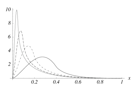
FIG. 5.: Nonforward parton distributions ${\cal F}_{\zeta}^{(1)}(X)$ for different values of the skewedness $\zeta=0.05$ (thin line), $\zeta=0.1$ (dashed line), $\zeta=0.2$ (dash-dotted line) and $\zeta=0.4$ (full line) in the “valence quark oriented” model specified by Eq.(6.11) for $a=0.5$.

                 
.                   $a)$                                $b)$                                $c)$                                $d)$

FIG. 6.: Ratio ${\cal F}_{\zeta}^{g}(X)/Xf_{g}(X)$ vs. $\log_{10}(X/\zeta)$ as obtained from the model given by Eq. (6.16) for $a)$ $\zeta=10^{-2},b)$ $\zeta=10^{-3},c)$ $\zeta=10^{-4}$ and $d)$ $\zeta=10^{-5}$ with $k=0.48$ (solid lines), $k=0.4$ (long-dashed lines) and $k=0.30$ (short-dashed lines).

FIG. 7.: Parton picture in terms of $a)$ modified double distributions and $b)$ off-forward parton distributions $H(\tilde{x},\xi)$.

                                       

FIG. 8.: Meson-like contribution.

REFERENCES

- [1] X. Ji, Phys.Rev.Lett. 78 610 (1997).
- [2] A.V. Radyushkin, Phys. Lett. B 380 (1996) 417.
- [3] X. Ji, Phys.Rev. D 55 (1997) 7114.
- [4] A.V. Radyushkin, Phys. Lett. B 385 (1996) 333.
- [5] A.V. Radyushkin, Phys. Rev. D 56 (1997) 5524.
- [6] S.J. Brodsky, L. Frankfurt, J.F. Gunion, A.H. Mueller and M. Strikman, Phys. Rev. D 50 (1994) 3134.
- [7] J.C. Collins, L. Frankfurt and M. Strikman, Phys. Rev. D 56 (1997) 2982.
- [8] D. Müller, D. Robaschik, B. Geyer, F.-M. Dittes and J. Hořejši, Fortschr.Phys. 42 (1994) 101.
- [9] L. Mankiewicz, G. Piller and T. Weigl, Eur.Phys.J. C 5 (1998) 119.
- [10] J. Blumlein, B. Geyer and D. Robaschik, DESY-97-209 (1997), hep-ph/9711405.
- [11] L. Frankfurt, A. Freund, V. Guzey and M. Strikman, Phys. Lett. B 418 (1998) 345.
- [12] J. Blumlein, B. Geyer and D. Robaschik, Phys. Lett. B 406 (1997) 161.
- [13] I.I. Balitsky and A.V. Radyushkin, Phys. Lett. B 413 (1997) 114.
- [14] Th. Braunschweig, B. Geyer and D. Robaschik, Ann. Phys. (Leipzig) 44 (1987) 403.
- [15] I.I. Balitsky and V.M. Braun, Nucl.Phys. B 311 (1988/89) 541.
- [16] A.V. Belitsky, B. Geyer, D. Müller and A. Schäfer, Phys. Lett. B 421 (1998) 312.
- [17] A.D. Martin and M.G. Ryskin, Phys. Rev. D 57 (1998) 6692.
- [18] K. Golec-Biernat, J. Kwiecinski and A.D. Martin, hep-ph/9803464.
- [19] A.V. Radyushkin, Phys. Lett. B 131 (1983) 179.
-
[20]
V.N. Gribov and L.N. Lipatov, Sov. J. Nucl. Phys.
15 (1972) 78;
L.N. Lipatov, Sov. J. Nucl. Phys. 20 (1975) 94. - [21] G. Altarelli and G. Parisi, Nucl. Phys. B 126 (1977) 298.
- [22] Yu. L. Dokshitser, Sov.Phys. JETP, 46 (1977) 641.
- [23] A.V. Efremov and A.V. Radyushkin, Theor. Math. Phys. 42 (1980) 97.
- [24] S.J. Brodsky and G.P. Lepage, Phys. Lett. B 87 (1979) 359.
- [25] X.Ji, J. Phys. G 24 (1998) 1181.
- [26] B. Pire, J. Soffer and O.V. Teryaev, hep-ph/9804284.
- [27] X. Ji, W. Melnitchouk and X. Song, Phys. Rev. D 56 (1997) 5511.
- [28] M. Glück, E. Reya and A. Vogt, Z. Phys. C 67 (1995) 433.
- [29] V.Yu. Petrov, P.V. Pobylitsa, M.V. Polyakov, I. Bornig, K. Goeke and C. Weiss, Phys. Rev. D 57 (1998) 4325.
- [30] I.V. Musatov and A.V. Radyushkin, work in progress.
- [31] S.V. Mikhailov and A.V. Radyushkin, Nucl. Phys. B273 (1986) 297.
- [32] M.K. Chase, Nucl. Phys. B174 (1980) 109.
- [33] M.A. Shifman and M.I. Vysotsky, Nucl.Phys. B 186 (1981) 475.
- [34] Th. Ohrndorf, Nucl. Phys. B 186 (1981) 153.
- [35] V.N. Baier and A.G. Grozin, Nucl. Phys. B 192 (1981) 476.
- [36] D.J. Gross and F. Wilczek, Phys. Rev. D 9 (1974) 980.
- [37] H. Georgi and H.D. Politzer, Phys. Rev. D 9 (1974) 416.
.