Domain Wall Production During Inflationary Reheating

Abstract

We numerically investigate the decay, via parametric resonance, of the inflaton with an $m^{2}\phi^{2}$ potential into a scalar matter field with a symmetry breaking potential. We consider the case where symmetry breaking takes place during inflation. We show that when expansion is not taken into account symmetry restoration and non-thermal defect production during reheating is possible. However in an expanding universe the fields do not spend sufficient time in the instability bands; thus symmetry restoration and subsequent domain wall production do not occur.

PACS numbers: 98.80Cq

BROWN-HET-1121, April 1998
FERMILAB-Pub-98/135-A

Introduction

The realisation that the decay of the inflaton might occur explosively, during a stage dubbed “pre-heating” [3, 4, 5] and lead to a universe far from thermal equilibrium, has a number of important ramifications. The most obvious is that the temperature of the universe, after thermalisation, may be much higher than under the old model of reheating. Another is the recent construction of a model for baryogenesis [6] which takes advantage of the out-of-equilibrium nature of the universe shortly after pre-heating. We, on the other hand, will be interested in the possibility of non-thermal phase transitions after pre-heating, and the possible production of topological defects.

This suggestion was first made by Kofman et al. [7], and Tkachev [8]. The essential idea is that pre-heating, via the mechanism of parametric resonance, typically gives rise to very large fluctuations in the fields and it is these that may restore a symmetry which has been broken by the time inflation ends. The important point is that symmetry restoration may occur even if the symmetry breaking scale is higher than the final reheat temperature. Then as the universe subsequently expands and cools, phase transitions will result in the creation of topological defects. This would be very intriguing. For a start we might find the re-emergence of a problem inflation was designed to solve, namely the monopole problem. The creation of domain walls would also be potentially problematic. However the production of strings may be a desirable feature of such scenarios, in that strings can be a seed for structure formation.

Khlebnikov et al. [9] have recently demonstrated that non-thermal defect production indeed occurs during inflationary reheating. They considered a model in which the inflaton field $\phi$ has a double well potential and is coupled to massless scalar matter fields $X_{i},i=1\ldots N$. Similar results (obtained from 2-D simulations) have also been shown by Kasuya and Kawasaki [10].

We study a different model. In our work the inflaton $\phi$ has a unique minimum and decays via parametric resonance into a scalar matter field $\chi$ with the discrete symmetry $\chi\rightarrow-\chi$. That is, we are interested in the question as to whether domain walls are produced. (Note that we are not considering a two-field model of inflation.) We assume that symmetry breaking occurs during inflation, for if it occurs afterwards the symmetry will then be restored a number of times by the oscillation of the inflaton alone, without any need for parametric resonance, and defect production will almost certainly ensue. This was pointed out by Kofman et al. in their original paper [7], where this model was first examined in the context of parametric resonance and defect production, and by Kofman and Linde in [11].

We investigate both the expanding and non-expanding cases and we show that symmetry restoration and defect production only occur in the non-expanding case. However the defects are not stable. Our work is based on 3-D lattice simulations, though we also understand the results from an analytical point of view.

The paper is set out as follows. We begin with a detailed explanation of the model including necessary constraints on the model. The second section is devoted to the analytical understanding of the model and predictions for the full simulation. After this we highlight the workings of the numerical code and present the results from our simulations. The final section is a brief summary of our study and conclusion.

1. Model

We consider the simplest model of inflation and reheating: the inflaton $\phi$ has potential $\frac{1}{2}m^{2}\phi^{2}$ and it decays into a second scalar field $\chi$. We let $\chi$ have the simplest potential which allows symmetry breaking: $\frac{1}{4}\lambda(\chi^{2}-\chi_{0}^{2})^{2}$, and suppose it interacts with $\phi$ through the interaction term: $\frac{1}{2}g^{2}\phi^{2}\chi^{2}$. Thus the full potential for the two-field theory is:

$$V(\phi,\chi)=\frac{1}{2}m^{2}\phi^{2}+\frac{1}{4}\lambda(\chi^{2}-\chi_{0}^{2})^{2}+\frac{1}{2}g^{2}\phi^{2}\chi^{2}\$$ (1)

The most important constraint on our model is the requirement that the symmetry breaking occurs during inflation. This is equivalent to demanding the interaction term in (1) not lift the degeneracy of the potential in the $\chi$ direction. As $\phi$ is homogeneous to a very good approximation for initial times, we may write $\phi\approx\phi(t)$ so that the effective potential for $\chi$ is:

$$V^{eff}_{\chi}=\frac{1}{4}\lambda(\chi^{2}-\chi_{0}^{2})^{2}+\frac{1}{2}g^{2}\phi^{2}(t)\chi^{2}\$$ (2)

This has degenerate minima if $\lambda\chi_{0}^{2}>g^{2}\phi(t)^{2}$. If this is true at $t=0$, then it is always true; for in the expanding case $\phi$ is redshifted to zero and in the non-expanding case $\phi$ is not observed to increase. If we define $\phi_{0}\equiv\phi(0)$, then the condition for degenerate minima becomes:

$$\lambda\chi_{0}^{2}>g^{2}\phi_{0}^{2}\$$ (3)

Another condition follows from the requirement that inflation proceed as usual, despite the presence of $\chi$. For this we must have the vacuum energy of $\chi$ to be much smaller than that of $\phi$:

$$\frac{1}{4}\lambda\chi_{0}^{4}\ll\frac{1}{2}m^{2}\phi_{0}^{2}\$$ (4)

When (4) is combined with (3), we obtain:

$$g^{2}\chi_{0}^{2}\ll m^{2}\$$ (5)

which ensures the frequency of oscillation of $\phi$ after inflation is dominated by $m$.

We next demand that the maximum reheat temperature be insufficient to lead to a thermally-corrected potential for $\chi$ with the degeneracy lifted. Since $T_{RH}<(m\,\phi_{0})^{\frac{1}{2}}$, this condition becomes:

$$\chi_{0}>(\frac{m}{\phi_{0}})^{\frac{1}{2}}\phi_{0}\$$ (6)

Actually the final reheat temperature will be many orders of magnitude smaller than we have indicated, so (6) is much stricter than it needs to be. However it is easy to satisfy and we will retain it in order to stress we are interested in non-thermal defect production.

Finally there are the usual constraints on $m$ and $g^{2}$ arising from the COBE data: $m\leq 10^{-6}M_{P}$ and $g^{2}\leq 10^{-6}$; the latter ensures radiative corrections do not lead to a too large self-coupling for $\phi$ (though in a supersymmetric model of inflation this condition may not be necessary [12]).

2. Analysis

Our working hypothesis is that parametric resonance will generate large fluctuations in $\chi$ which will restore the symmetry of the $\chi$-field in some regions of space. After this, in such regions, $\chi$ may evolve into the two degenerate minima of its potential, possibly forming a stable domain wall. In other words, we expect the mechanism of parametric resonance will be able to channel sufficient energy from the inflaton into the $\chi$-field in order to drive $\chi$ over the potential barrier. In this section we outline the conditions for effective parametric resonance, considering both the expanding and non-expanding cases.

We begin by assuming the usual flat FRW universe, in co-moving co-ordinates:

$$ds^{2}=dt^{2}-a^{2}(t)(dx^{2}+dy^{2}+dz^{2})$$ (7)

To a good approximation the coherent oscillations of the inflaton rapidly give rise to a matter dominated universe so we may write: $a(t)=(1+mt)^{\frac{2}{3}}$, where $t=0$ is the time at the end of inflation and we have used our freedom to scale the spatial co-ordinates to impose $a(0)=1$. If we put: $a(t)=(1+mt)^{n}$, we can simultaneously consider the non-expanding case ($n=0$) and the expanding case ($n=\frac{2}{3}$).

The equations of motion for the fields $\phi$ and $\chi$ are the standard ones for scalar fields in a curved space-time with minimal coupling to gravity:

$$\ddot{\phi}+3H\dot{\phi}-a^{-2}\nabla^{2}\phi+(m^{2}+g^{2}\chi^{2})\phi=0$$ (8)

$$\ddot{\chi}+3H\dot{\chi}-a^{-2}\nabla^{2}\chi+(\lambda(\chi^{2}-\chi_{0}^{2})+g^{2}\phi^{2})\chi=0$$ (9)

where $H\equiv\frac{\dot{a}}{a}$.

These are the equations which are solved in our numerical simulation. Here we point out that in our simulation the scale factor $a(t)$ is put in by hand, rather than determined in a self-consistent manner.

The initial conditions for $\phi$ are those of the end of inflation i.e. when the slow roll approximation is no longer valid. We find: $\phi(0)\equiv\phi_{0}=\frac{1}{\sqrt{3\pi}}M_{P}$ and $\dot{\phi}(0)=-m\,\phi_{0}$. In addition we chose $m=10^{-6}\phi_{0}$. For the non-expanding case we will assume $\dot{\phi}(0)=0$. As for $\chi$, inflation dictates it will be initially comprised of quantum fluctuations about one of the instantaneous minima of $V^{eff}_{\chi}$, which are given by $\chi_{\pm}(t)\equiv\pm\chi_{0}\,\surd(1-\frac{g^{2}\phi^{2}(t)}{\lambda\chi_{0}^{2}})$. Without loss of generality we may choose the positive minimum.

To make headway in our analytical understanding of the model we must make some simplifying approximations. As already noted, we may take $\phi$ to be homogeneous to start with. Recalling (5), this allows us to solve (8): $\phi=\phi_{0}\,a(t)^{-\frac{3}{2}}\cos{mt}$, and to re-write (9) as:

$$\ddot{\chi}+3H\dot{\chi}-a^{-2}\nabla^{2}\chi+\frac{\partial}{\partial\chi}V^{eff}_{\chi}=0\$$ (10)

In order to understand the evolution of the $\chi$-field, at least initially, we will expand $V^{eff}_{\chi}$ to quadratic order about $\chi_{+}(t)$:

$$V^{eff}_{\chi}\longrightarrow U_{\chi}=\lambda\chi_{+}^{2}(t)(\chi-\chi_{+}(t))^{2}+\frac{1}{4}\lambda(\chi_{0}^{4}-\chi_{+}^{4}(t))\$$ (11)

How now do we ask if symmetry restoration occurs? We note that $U_{\chi}(\frac{1}{2}\chi_{+}(t))=\frac{1}{4}\lambda\chi_{0}^{4}$, which is the barrier height of $V^{eff}_{\chi}$. Thus the question as to whether $\chi$ surmounts the potential barrier of $V^{eff}_{\chi}$ may be replaced with the question: does $\chi$, evolving under the influence of $U_{\chi}$, ever become less than $\frac{1}{2}\chi_{+}(t)$?

With the substitution of $V^{eff}_{\chi}$ with $U_{\chi}$ in (10), we obtain a linear equation for $\chi$. Upon rescaling: {$t\rightarrow\frac{t}{m},\ {\bf x}\rightarrow\frac{{\bf x}}{m},\ \phi\rightarrow\phi_{0}\phi,\ \chi\rightarrow\phi_{0}\chi,\ g^{2}\rightarrow(\frac{m}{\phi_{0}})^{2}\,g^{2},\ \lambda\rightarrow(\frac{m}{\phi_{0}})^{2}\,\lambda$}, taking the Fourier transform and introducing $X_{{\bf k}}\equiv a^{\frac{3}{2}}\,\chi_{{\bf k}}$, we arrive at a Mathieu equation with (in general) time-dependent co-efficients, for the non-zero momentum modes $X_{{\bf k}}$:

$$\ddot{X}_{{\bf k}}+(A_{k}(t)-2q(t)\cos{2t})\,X_{{\bf k}}=0$$ (12)

where $A_{k}=\frac{k^{2}}{a^{2}}+2\lambda\chi_{0}^{2}-\frac{g^{2}}{a^{3}}$ and $q=\frac{g^{2}}{2a^{3}}$.

The existence of exponentially growing, or unstable solutions to the Mathieu equation is well known and, in physics literature, has been termed parametric resonance. However recent work [14, 15, 16], inspired by the pre-heating scenario, has led to new insight into the nature of these solutions. For time-independent coefficients, we may identify three different regions of instability. (i) Narrow band resonance: $A_{k}\simeq l^{2}\geq 2q$, $l=1,2\ldots$ and $q\ll 1$. The solution $X_{{\bf k}}$ oscillates with period $2\pi$, and is modulated by an exponential function, $e^{\mu_{k}t}$, where $\mu_{k}$ is called the characteristic exponent or growth index. Typically $|\mu_{k}|\sim\frac{q}{2}$. (ii) Broad band resonance: $A_{k}\geq 2q$ and $q\gtrsim 1$. The solution oscillates many times faster than in the narrow band case and grows in exponential jumps, occurring at time intervals of $\pi$. The overall growth index may also be much larger: one finds $|\mu_{k}|<0.3$. (iii) Negative instability: $A_{k}<2q$. The solutions in this region are almost all unstable and $|\mu_{k}|>1$ is possible. Recently Greene et al. [16] have constructed a model which makes use of this region.

The situation of the Mathieu equation with time-dependent coefficients is much more complicated. The difficulty is that, during one oscillation of the driving force, $X_{{\bf k}}$ does not remain in one instability band but in fact passes in and out of many such bands. The result is that parametric resonance becomes essentially haphazard—$X_{{\bf k}}$ may even decrease in amplitude at times—and hence the term stochastic resonance has been applied to this scenario. However exponential type growth is still possible, and the work of Kofman et al. [15] has done much to clarify this issue.

Returning to equation (12), we see that in our case $A_{k}$ is always greater than $q$ because of (3), hence we will only see broad band or narrow band resonance. A necessary condition for parametric resonance [15] in these regions is:

$$\kappa^{2}\equiv\frac{A_{k}-2q}{2\sqrt{q}}\leq 1\$$ (13)

It is useful to introduce the dimensionless parameters: $\alpha=g^{2}$, $\beta=\lambda\chi_{0}^{2}$ and $\gamma=\chi_{0}^{-2}$. Then conditions (3), (4) and (6) may be succinctly written: $\alpha<\beta\ll\gamma\lesssim 10^{6}$.

For $n=\frac{2}{3}$, $\kappa^{2}\rightarrow\frac{\sqrt{2}\beta}{\sqrt{\alpha}}\,t$ which must always become larger than $1$. Later we will see that the typical time for symmetry restoration to begin in the non-expanding case is $t\sim 30$. Thus to satisfy (13) in the expanding case we will require $\sqrt{\alpha}\gg\beta$. But $\alpha<\beta$. So we must have:

$$\sqrt{\alpha}\ll 1$$ (14)

Or in other words, $g^{2}_{phys}\ll 10^{-12}$. We conclude that if (14) is not satisfied, and we believe it is not in any realistic model, then the system is not long enough in the instability regions to restore the symmetry. The conclusion is further reinforced if we realise we also require $\mu_{k}>\frac{3}{2}H$, but that initially $\frac{3}{2}H(0)=1>0.3\sim\mu_{k,max}$.

The necessary condition for parametric resonance in the case of $n=0$ is much less stringent. (13) gives:

$$\beta\leq\alpha+\sqrt{\frac{\alpha}{2}}$$ (15)

A test of the validity of our approximation in the non-expanding case is the time taken for symmetry to start being restored. As mentioned previously, what we need to calculate is the time at which $\chi$ first becomes less than $\frac{1}{2}\chi_{+}(t)$. The modes in the resonance band will dominate the behaviour of $\chi$ so:

$$\chi \approx \frac{1}{(2\pi)^{\frac{3}{2}}}\,\frac{m}{\phi_{0}}\int_{res.\ band}d^{\,3}k\,\chi_{{\bf k}}\,e^{-i\,{\bf k}.{\bf x}}$$ (16)

$$\sim \frac{1}{(2\pi)^{\frac{3}{2}}}\,\frac{m}{\phi_{0}}\,.\,4\pi\,k^{2}_{res}\,\frac{\Delta k}{2}\,|\chi_{{\bf k},res}|$$ (17)

$$\approx \frac{k^{2}_{res}\,\Delta k}{(2\pi)^{\frac{1}{2}}}\,\frac{m}{\phi_{0}}\,\frac{e^{\,\mu_{k}t}}{\sqrt{\,\omega_{res}}}$$ (18)

where $\Delta k$ is the width of the resonance band and $\omega^{2}_{res}\equiv A_{k,res}-2q\cos{2t}=k^{2}_{res}+2\beta-\alpha-\alpha\cos{2t}$. The appearance of $\frac{m}{\phi_{0}}$ and $\sqrt{\,\omega_{res}}$ is due to $\chi$ starting out as quantum fluctuations [17].

Typically in our parameter range, we find a region of broad band resonance for $\beta$ slightly greater than $\alpha$, with $k_{res}\sim\Delta k\sim 1$ and $\mu_{k}\sim 0.25$. Then the statement $\chi\leq\frac{1}{2}\chi_{+}(t)$ becomes $\frac{m}{\phi_{0}}\,\beta^{-\frac{1}{4}}\,e^{\,\mu_{k}t}\lesssim\chi_{0}$, which implies:

$$t\gtrsim 4\ln{(10^{6}\beta^{\frac{1}{4}}\gamma^{-\frac{1}{2}})}\sim 30$$ (19)

To summarise: our analysis suggests that in the non-expanding case the conditions for parametric resonance depend only on $\alpha$ and $\beta$, whereas the time taken for parametric resonance to restore the symmetry of the $\chi$-field is determined mainly by $\gamma$. In the expanding case we do not expect domain walls to be produced. We now turn to the full simulation of the two-field system.

3. Simulation and Results

The classical equations of motion (8) and (9) are a good approximation to the behaviour of an actual matter field, $\chi$, coupled to the inflaton, provided the mode amplitudes of $\chi$ are large. Although initially these are taken to be quantal fluctuations, the modes we are interested in are in the resonance band and hence they quickly grow and become classical [18].

We work in terms of the rescaled, non-dimensional quantities of the previous section. The universe becomes the usual 3-dimensional lattice in co-moving co-ordinate space, and we apply periodic boundary conditions. The fields are evolved using a leap-frog scheme, which is an explicit algorithm second-order accurate in time. The spatial derivatives are evaluated to fourth-order accuracy.

The results presented here were obtained on $64^{3}$ lattices, though we also checked representative cases on $128^{3}$ lattices. We varied the lattice spacing, the only proviso being that we remained sensitive to the momentum modes in the expected resonance bands, and obtained essentially identical data. The total energy of the system was conserved to better than $0.1\%$. Two other tests convinced us of the accuracy of our simulation: we were able to repeat the results of [19], and, in an $O(2)$ $\chi$-field simulation, we found a faithfully modelled, collapsing string loop.

A brief note about the determination of the initial conditions for $\chi$ is warranted. As mentioned before, we treat $\chi$ initially as quantum fluctuations about one of the instantaneous minima of its potential. One may think of the quantum fluctuations in momentum space as an infinite collection of harmonic oscillators (with time dependent frequencies in this case) [20]. Our approach essentially was to pick the occupation numbers of the modes on the lattice randomly from a Gaussian distribution with $k$-dependent width [17]. We also included a random phase and then inverse Fourier transformed to obtain $\chi$ in configuration space. We checked that our results were not sensitively dependent on the particular random numbers chosen. A final important point is that the lattice spacing gives a natural cutoff to the high momentum modes, and one must choose this so that $E_{fluct.}\ll E_{inflaton}$.

We examined the region in parameter space of $\alpha,\beta\sim 100$ and $\gamma\sim 10^{4}$; in other words $g_{phy}^{2}\sim 10^{-10},\lambda_{phy}\sim 10^{-6}$ and $\chi_{0,phy}\sim 0.01\phi_{0}\approx 3\times 10^{16}$ GeV. The choice of these parameters was partially determined by the requirements that we be sensitive to the instability bands and the box be large enough to include any defects produced [22]. The numerical parameters were: lattice spacing $\Delta x=0.1-1$ and time step $\Delta t=0.02$.

The first result is that we did not find any evidence of symmetry restoration in an expanding universe. In all cases we considered, $\chi\rightarrow\chi_{0}$ and $\phi$ merely redshifted to 0. This is as predicted by (14) and Kofman et al. [7].

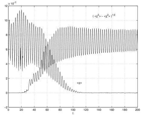
FIG. 1.: The mean and variance of $\chi$ in time ($\alpha=100$, $\beta=130$ and $\gamma=10^{4}$).

The non-expanding scenario is more interesting however. Figure 1 shows the behaviour of $\langle\chi\rangle$ and $\surd(\langle\chi^{2}\rangle-\langle\chi\rangle^{2})$ for $\alpha=100$, $\beta=130$ and $\gamma=10^{4}$. This is typical of the cases in which symmetry is restored: the mean value of $\chi\rightarrow 0$ and the fluctuations grow to be of the order of $\chi_{0}$. Also typical is the fact that the back-reaction of $\chi$ on $\phi$ is very slight. $\langle\phi\rangle$ continues to oscillate sinusoidally and the fluctuations of $\phi$ are only of order $3\times 10^{-3}\ll 1$ at $t=200$.

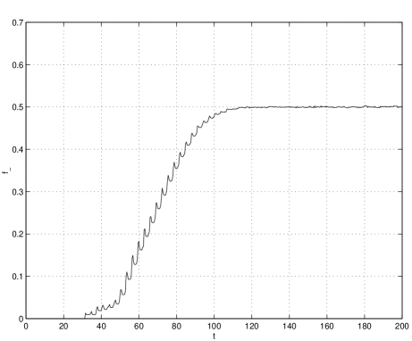
FIG. 2.: The fraction of the volume with $\chi<0$ ($\alpha=100$, $\beta=130$ and $\gamma=10^{4}$).

Plotted in figure 2 is the fraction, $f_{-}$, of the volume of the box with $\chi<0$. The jumps in $f_{-}$ occur at intervals of $\pi$ which is as expected; $\pi$ is the period of the driving term in the Mathieu equation i.e. $\phi^{2}$. Note too the onset of symmetry restoration is at $t\approx 30$, confirming our earlier order of magnitude estimate. However, considering all our runs, we did not find agreement with the specific form of (19). (Usually $t=15-80$.) On the other hand varying $\gamma$, for fixed $\alpha$ and $\beta$, did not alter whether symmetry was or was not restored, as was our prediction.

In the non-expanding case, symmetry restoration (when it occurs) gives rise to non-thermal production of defects. However these defects are not stable. This can be seen in our simulations: the regions of $\chi<0$ are essentially randomly scattered throughout the box (even when they account for half the volume of the box) and percolate. In addition they are uncorrelated in time.

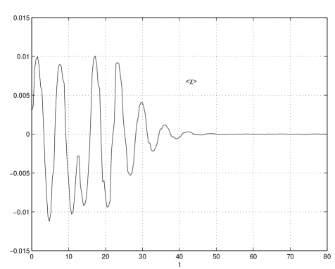
FIG. 3.: The mean of $\chi$ in time ($\alpha=100$, $\beta=110$ and $\gamma=10^{4}$).

There is one problem with the particular case we have been considering above: it does not satisfy (15). Thus the analysis of section 2 cannot be entirely correct. Figures 3 and 4 detail what was an unexpected result but which led to a more complete understanding of our model. Here $\alpha=100$, $\beta=110$ and $\gamma=10^{4}$. Clearly what is happening is an initial series of global sign changes, prior to eventual local symmetry restoration. The change in sign is not important because the symmetry of $\chi$ remains broken, but it does indicate we were naive to imagine $\chi$ would fluctuate about $\chi_{+}(t)$ for early times.

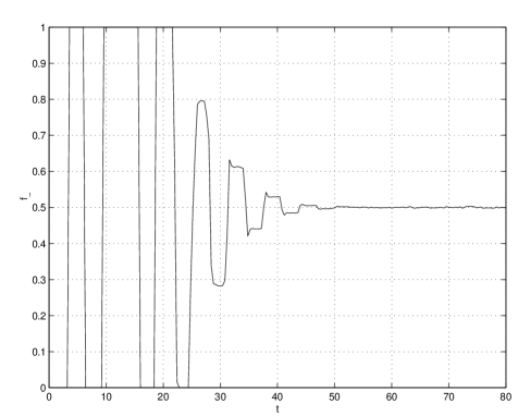
FIG. 4.: The fraction of the volume with $\chi<0$ ($\alpha=100$, $\beta=110$ and $\gamma=10^{4}$).

It is more appropriate to put $\chi({\bf x},t)=\chi_{h}(t)+\delta\chi({\bf x},t)$, where $\chi_{h}$ satisfies the homogeneous version of (10). Then the linearised equation for $X_{{\bf k}}\equiv a^{\frac{3}{2}}\delta\chi_{{\bf k}}$, which replaces (12), is:

$$\ddot{X}_{{\bf k}}+(\frac{k^{2}}{a^{2}}+\lambda(\,3\chi_{h}^{2}(t)-\chi_{0}^{2})+g^{2}\phi^{2}(t))\,X_{{\bf k}}=0$$ (20)

The behaviour of $\chi_{h}$ is quite delicate. Numerical solution of its ODE shows that for early times it is true $\chi_{h}\approx\chi_{+}$, except when $\beta\approx\alpha$ where we find $\chi_{h}\approx\pm\chi_{+}$. This is the sign change seen in figures 3 and 4. At later times $\chi_{h}^{2}$ typically oscillates about $\chi_{+}^{2}$, with a frequency several times greater than that of the inflaton. For $n=\frac{2}{3}$, $\chi_{h}^{2}\rightarrow\chi_{+}^{2}\rightarrow\chi_{0}^{2}$  so in this case we believe our earlier analysis is essentially unchanged. However for $n=0$, $\chi_{h}^{2}$ tends to increase in amplitude. This ruins a straight-forward analysis in terms of a Mathieu equation for $X_{{\bf k}}$ (which would come about if $\chi_{h}^{2}=\chi_{+}^{2}$). Numerical analysis of (20) for $n=0$ though does reveal exponential-type solutions. In fact parametric resonance appears to be much more likely: the instability bands are larger than those of the broad band regime of the Mathieu equation. We are currently working on an analytical understanding of these results[22].

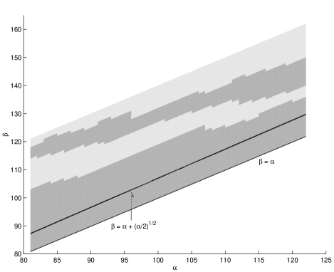
FIG. 5.: The region of symmetry restoration (darker shading) in the $\alpha-\beta$ plane.

To conclude this section figure 5 shows the region of the $\alpha-\beta$ plane we investigated where symmetry restoration occurs, for the non-expanding case. We stress that this plot is an extrapolation from 45 simulations we performed, and as such to be taken only as a rough guide. However it indicates two features which we are certain about. Firstly the existence of band structure. This is reminiscent of the Mathieu equation instability bands, even down to their relative sizes. Secondly the fact that as $\beta$ increases for fixed $\alpha$, symmetry restoration is no longer possible. From this graph we conservatively deduce a condition for symmetry restoration:

$$\beta<2\,\alpha$$ (21)

Also shown in figure 5 is our prediction from section 2. The discrepancy is the most striking evidence that our earlier analysis was inadequate.

4. Conclusions

We have numerically investigated the decay of the inflaton into a scalar matter field $\chi$ with a symmetry breaking potential, when the symmetry is broken during inflation. In the non-expanding case we found that symmetry restoration is possible via parametric resonance. The analysis is complicated but interestingly the regions of instability are much larger than those of the Mathieu equation. This situation of more efficient parametric resonance has also been seen in the work of Zanchin et al. [21]. We think it would be useful to more fully understand equations like (20), perhaps utilising the methods of [15]. Finally we found that non-thermal defect production occurs, but that the defects are not stable.

In the expanding case we found that domain wall production did not take place. This leads us to conclude that the inflaton may safely couple to $\chi$ with the potential as in (1). Actually the precise form for the potential may be unimportant. Recall that the symmetry of $\chi$ is broken before the end of inflation. In fact, if there are to be no fluctuations due to the initial symmetry breaking in our Hubble volume, the symmetry must be broken early enough to allow for the usual number of $e$-foldings by the time inflation is over. In our model this means $\beta\gtrsim 100\,\alpha$[22] which is to be compared with (21). This amounts (literally) to a very formidable barrier to symmetry restoration. This suggests it is unlikely that there will be defect production in any realistic model in which $\chi$ has the symmetry breaking potential and the symmetry is broken during inflation.

Acknowledgements

It is a pleasure to be able to thank Tomislav Prokopec, Richard Easther, Guy Moore and Martin Götz who were helpful at crucial stages. In particular we would like to thank Anne-Christine Davis who initially jump-started this investigation, Robert Brandenberger who was a continual source of help, and Andrei Linde who more than once gave one of us (MP) pertinent advice. Computational work in support of this research was performed at the Theoretical Physics Computing Facility at Brown University. This work was supported by the DOE and the NASA grant NAG 5-7092 at Fermilab.

REFERENCES

- [1] Email: parry@het.brown.edu
- [2] Email: ats@traviata.fnal.gov
- [3] J. Traschen and R. Brandenberger, Phys. Rev. D42, 2491 (1990)
- [4] L. Kofman, A. D. Linde and A. A. Starobinskii, Phys. Rev. Lett. 73, 3195 (1994)
- [5] Y. Shtanov, J. Traschen and R. Brandenberger, Phys. Rev. D51, 5438 (1995)
- [6] E. W. Kolb, A. Riotto and I. I. Tkachev, hep-ph/9801306
- [7] L. Kofman, A. D. Linde and A. A. Starobinskii, Phys. Rev. Lett. 76, 1011 (1996)
- [8] I. I. Tkachev, Phys. Lett. B376, 35 (1996) (1997)
- [9] S. Khlebnikov, L. Kofman, A. Linde and I. Tkachev, hep-ph/9804425
- [10] S. Kasuya and M. Kawasaki, hep-ph/9804429
- [11] L. Kofman and A. D. Linde, Nucl. Phys. B282, 555 (1987)
- [12] A. D. Linde, private communication
- [13] F. M. Arscott, “Periodic Differential Equations”, (The MacMillan Company, New York 1964)
- [14] L. Kofman, astro-ph/9605155
- [15] L. Kofman, A. D. Linde and A. A. Starobinskii, Phys. Rev. D56, 3258 (1997)
- [16] B. Greene, T. Prokopec and T. G. Roos, Phys. Rev. D56, 6484 (1997)
- [17] S. Yu. Khlebnikov and I. I. Tkachev, Phys. Lett. B390, 80 (1997)
- [18] S. Yu. Khlebnikov and I. I. Tkachev, Phys. Rev. Lett. 77, 219 (1996)
- [19] T. Prokopec and T. G. Roos, Phys. Rev. D55, 3768 (1997)
- [20] R. Brandenberger, Nucl. Phys. B245, 328 (1984)
- [21] V. Zanchin, A. Maia, Jr., W. Craig and R. Brandenberger, Phys. Rev. D57, 4651 (1998)
- [22] M. F. Parry and A. T. Sornborger, in preparation