[

Cosmic strings from preheating

Abstract

We investigate nonthermal phase transitions that may occur after post-inflationary preheating in a simple model of a two-component scalar field with the effective potential $\lambda(\phi_{i}^{2}-{\rm v}^{2})^{2}/4$, where $\phi_{1}$ is identified with the inflaton field. We use three-dimensional lattice simulations to investigate the full nonlinear dynamics of the model. Fluctuations of the fields generated during and after preheating temporarily make the effective potential convex in the $\phi_{1}$ direction. The subsequent nonthermal phase transition with symmetry breaking leads to formation of cosmic strings even for ${\rm v}\gg 10^{16}$ GeV. This mechanism of string formation, in a modulated (by the oscillating field $\phi_{1}$) phase transition, is different from the usual Kibble mechanism.

PACS: 98.80.Cq          PURD-TH-98-07,  UH-IfA-98-30,  SU-ITP-98-32          hep-ph/9805209

This paper is dedicated to the memory of David Abramovich Kirzhnits

]

The theory of cosmological phase transitions proposed in 1972 by David Kirzhnits gradually became one of the most essential parts of modern cosmology [1]. Originally it was assumed that such phase transitions occur in a state of thermal equilibrium when the temperature decreased in the expanding universe. Recently it was found that large fluctuations of scalar and vector fields produced during preheating after inflation [2] may lead to specific nonthermal phase transitions which occur far away from the state of thermal equilibrium [3]. To investigate these phase transitions one should study the self-consistent nonlinear dynamics of quantum fluctuations amplified by parametric resonance. This is a very complicated task. Fortunately, fluctuations of Bose fields generated during preheating have very large occupation numbers and can be considered as interacting classical waves, which allows one to perform a full study of all nonlinear effects during and after preheating using lattice calculations [4]. These calculations, as well as analytical estimates [2, 3, 4, 5, 6, 7, 8] have already shown that fluctuations can grow large enough for cosmologically interesting phase transitions to occur. Lattice calculations can be used to directly simulate nonthermal phase transitions and formation of topological defects. This made it possible to go beyond the early attempts to study such phase transitions numerically [9], which neglected crucial backreaction effects beyond the Hartree approximation.

We made a series of lattice simulations of nonthermal phase transitions, focusing primarily on the possibility of generation of topological defects [10, 11]. The model with one scalar field with the potential $\lambda(\phi^{2}-{\rm v}^{2})^{2}/4$ has a broken discrete symmetry $\phi\rightarrow-\phi$. In this model we have found formation of domain structure [10]. If the inflaton field $\phi$ strongly couples to another scalar field $\chi$, the phase transition is strongly first order; we observed formation of bubbles of the new phase [11].

In this Letter we will study string formation in the theory of a two-component scalar field $\phi_{i}$ with the effective potential $\lambda(\phi^{2}-{\rm v}^{2})^{2}/4$, where $\phi^{2}=\sum\phi_{i}^{2}$. This model has $O(2)$ rotational symmetry and allows for string formation [10] (for early conference reports see [12]). Recently Kasuya and Kawasaki reported formation of defects in 2d lattice simulations for ${\rm v}\lesssim 3\times 10^{16}$ GeV [13], which confirmed our general conclusion concerning the phase transition in this model [10, 12]. However, scattering of particles, as well as the nature of topological defects in two dimensions and in three dimensions are quite different. In particular, there are no strings in this model in two dimensions. We have found that in the realistic case of three dimensions the generation of fluctuations is much more effective, and string production is possible even if ${\rm v}$ is as large as $6\times 10^{16}$ GeV.

In the model with the two-component field $\phi_{i}$ we can always rotate fields in such a way that initially $\phi_{2}=0$, and the field $\phi_{1}$ plays the role of the classical oscillating inflaton field. We denote by $\phi(0)$ the value of the field $\phi_{1}$ at the moment when inflation ends and the inflaton field begins to oscillate. It is convenient to work with the rescaled conformal time $\tau$, where $\sqrt{\lambda}\phi(0)dt=a(\tau)d\tau$, $a(0)=1$, and perform conformal transformation of the fields, $\varphi=\phi(\tau)a(\tau)/\phi(0)$. We also will use the rescaled spatial coordinates ${\bf x}\to\sqrt{\lambda}\phi(0){\bf x}$. The initial conditions at the beginning of preheating are determined by the preceding stage of inflation. We define the beginning of preheating as the moment $\tau=0$ when the velocity of the field $\phi$ in conformal time is zero. This happens when $\phi(0)\approx 0.35M_{\rm Pl}$ and $a(\tau)\approx 0.51\tau+1$ [4].

In the new variables, the equations of motion become

$${\ddot{\varphi}_{i}}-\nabla^{2}\varphi_{i}+(\varphi^{2}-v^{2}a^{2})\varphi_{i}=0\;,$$ (1)

where ${v}={\rm v}/\phi(0)$. Equation (1) contains only one parameter, ${v}$. The coupling constant $\lambda$ is hidden in the initial conditions for fluctuations; these were chosen as described in Ref. [4].

The full nonlinear equations of motion (1) were solved numerically directly in the configuration space. The computations were done on $128^{3}$ lattices with the box size $L=16\pi$, with the expansion of the universe assumed to be radiation dominated. There are several important quantities that can be measured in the simulations during the evolution of the system. One can define the zero mode $\varphi_{0i}=\langle\varphi_{i}(x,\tau)\rangle$ for each of the components $i=1,2$ of the field $\varphi$, and variances $\langle(\delta\varphi_{i})^{2}\rangle$, which measure the average magnitude of fluctuations $\delta\varphi_{i}=\varphi_{i}(x,\tau)-\varphi_{0i}$. Since the system is homogeneous on large scales, averages in these relations can be understood as volume averages. This is equivalent to taking an average over realizations of the initial data (the ensemble average). The averaged quantities depend only upon time and do not depend upon spatial coordinates ${\bf x}$.

We performed calculations for various ${\rm v}$ and $\lambda$. In the beginning we present results for ${\rm v}=3\times 10^{16}$ GeV and $\lambda=10^{-12}$. In the last part of the paper we also present result for different values of ${\rm v}$ and for $\lambda=10^{-13}$. The behavior of the zero modes $\phi_{0i}=\langle\phi_{i}\rangle$, and of the variances, ${\langle(\phi_{i}-\phi_{0i})^{2}\rangle}$, for each of the field components is shown in Fig. 1.

FIG. 1.: Variances of the field components $\phi_{2}$ and $\phi_{1}$ (upper and lower solid curves respectively) as well as the zero modes of these fields (upper dotted curve is $\langle\phi_{1}\rangle$ and lower dotted curve is $\langle\phi_{2}\rangle$) are shown as functions of conformal time.

Let us explain the evolution of the fluctuations. For such a small value of ${\rm v}$, preheating is completed at $\tau\approx 100$, well before the phase transition with symmetry breaking, which occurs at $\tau\approx 240$. During the stage of parametric resonance $\tau\leq 100$, the term $v^{2}a^{2}$ in (1) can be neglected. The equations for the mode functions of fluctuations in the directions of $\phi_{1}$ and $\phi_{2}$ are

$$\ddot{\varphi}_{ik}+(k^{2}+q_{i}\varphi_{01}^{2})\varphi_{ik}=0\,,$$ (2)

where the background inflaton oscillations $\varphi_{01}(\tau)$ are given by an elliptic function. The resonance parameter is different for different components: $q_{1}=3$ and $q_{2}=1$. For both components there is a single instability band, but the locations of the bands and the strengths of the resonance are different [14]. The resonance in the “inflaton” direction $\varphi_{1}$ is weak, the maximal value of the characteristic exponent of the fluctuations $\varphi_{1k}\propto e^{\mu_{1}\tau}$ is $\mu_{1}\approx 0.036$; the resonance in the perpendicular direction $\varphi_{2}$ is much stronger and broader, $\mu_{2}\approx 0.147$.

However, the actual growth rate of the fluctuations $\varphi_{1k}$ is not smaller but larger than that of the $\varphi_{2k}$ fluctuations. Indeed, the cross-interaction term $\varphi^{2}_{1}\varphi^{2}_{2}$ leads to the production of $\delta\varphi_{1}$ fluctuations in the process of rescattering [6]. As a result, the amplitude $\varphi_{1,k}$ grows as $\varphi_{1k}\propto e^{2\mu_{2}\tau}$, where $2\mu_{2}=0.294$ [12], as clearly seen in Fig. 1. This growth is much faster than in the 2d lattice simulations of Ref. [13].

We see that during the time interval between completion of preheating and the phase transition, $100\lesssim\tau\lesssim 240$, the zero mode of $\phi_{1}$ decreases faster than the variances (both are decreasing due to the expansion of the universe, but in addition the zero mode continues to decay into field fluctuations), and by the time $\tau\approx 240$ the field variance is as big as its zero mode.

FIG. 2.: Time dependence of the zero mode of $\phi_{1}$.

Time interval $100\lesssim\tau\lesssim 240$ is dominated by rescattering of all modes [4]. During this time interval, the symmetry (at least in one direction) is restored by large fluctuations. To see this, we study the time dependence of the zero mode of $\phi_{1}$, which is shown in Fig. 2. We immediately see some peculiarity. In the potential of the form $(\phi^{2}-{\rm v}^{2})^{2}$ the field cannot oscillate near $\phi=0$ with amplitude smaller than $\phi_{c}\equiv\sqrt{2}{\rm v}$. This critical value of the amplitude is shown in Fig. 2 by the dashed line, and we see that the field does oscillate with an amplitude smaller than $\phi_{c}$. At some point, the amplitude of the oscillations even becomes smaller than ${\rm v}$, i.e. the field is oscillating on the top of the tree potential without rolling down to its minimum. This means that the tree potential is significantly altered by the interaction with the background of created fluctuations, and the symmetry is restored.

We can reconstruct the effective potential $V_{\rm eff}(\varphi)$ using the already calculated function $\varphi_{0i}(\tau)=\langle\varphi_{i}\rangle$ and the definition

$${\ddot{\varphi}_{0i}}+dV_{\rm eff}/d\varphi_{0i}=0\;.$$ (3)

This definition of the effective potential is perfectly legitimate in the case when corrections to terms with the time derivative are small, which appears to be the case. (Expansion of the universe will be properly included when we work in the conformal coordinates, as in Eq. (3), and then “rotate” potential back to the synchronous frame and to the original fields.) This method allows one to find $V_{\rm eff}$ up to a constant. The reconstruction along $\varphi_{1}$ direction is shown for several moments of time in Fig. 3. At $\tau\approx 90$ the effective potential, shown by dots, coincides to a very good accuracy with the tree potential, shown by the solid line. This moment is not far away from the end of the exponential growth of fluctuations, which occurs at $\tau\approx 100$, but fluctuations at $\tau\approx 90$ are still rather small. At $\tau\approx 110$ fluctuations are large, and the effective potential is completely different: it has only one minimum. Note that the potential is slightly asymmetric with respect to the change of sign of the field $\phi_{1}$. This happens because in our simulations we are sampling the effective potential in the time-dependent background, when the points with positive and negative $\phi$ correspond to different moments of time. The “instantaneous” potential would be exactly symmetric, with a minimum at $\phi_{1}=0$, and symmetry is restored, at least in the $\phi_{1}$ direction.

FIG. 3.: Reconstruction of the effective potential in $\phi_{1}$ direction at several moments of time. Dots correspond to $\tau\approx 90$, diagonal crosses to $\tau\approx 110$, larger stars to $\tau\approx 180$ and smaller stars to $\tau\approx 215$. Solid line is the tree potential.

Still, the existence of an oscillating zero mode $\phi_{1}$ implies that symmetry between states with $\phi_{1}>0$ and $\phi_{1}<0$ is not exact. Thus one wonder whether one can say that symmetry is restored if the effective potential has the minimum at $\phi_{1}=0$, or one should not say so until the amplitude of oscillations of the field $\phi_{1}$ completely vanishes.

In our opinion, if the effective potential has a minimum at $\phi_{1}=0$, this implies that there is no spontaneous symmetry breaking, so in this sense the symmetry $\phi_{1}\to-\phi_{1}$ is restored. From a more pragmatic point of view, the issue of symmetry restoration and subsequent symmetry breaking is important mainly because it is related to production of topological defects. Therefore instead of debating which definition of symmetry restoration is better, we will try to find whether the topological defects are produced. Indeed we will see that cosmic strings are produced as a consequence of preheating.

At $\tau\approx 240$ the field fluctuations become diluted by the expansion of the universe to the extent sufficient for symmetry breaking. This event can be seen both in Fig. 1 and in Fig. 2. At that time, the zero mode nearly vanishes. This happens not because of symmetry restoration, but because the field rolls down to the $O(2)$ symmetric valley of minima of the effective potential in all possible directions in the field space, which, after averaging, gives $\langle\phi_{1}\rangle\ll{\rm v}$.

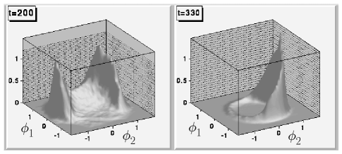
FIG. 4.: The joint probability distribution function of $\phi_{1}$ and $\phi_{2}$ before and after the phase transition. Fields $\phi_{1}$ and $\phi_{2}$ are shown in units of ${\rm v}$.

A useful quantity to consider is the probability distribution function $P(\phi_{1},\phi_{2},t)$ shown in Fig. 4. The first of these two figures shows that at $\tau\sim 200$ the maximum of the probability distribution oscillates near $\phi_{1}=0$ in the $\phi_{1}$ direction. This distribution has only one maximum in the $\phi_{1}$ direction. When this maximum approaches $\phi_{1}=0$, the distribution $P(\phi_{1},\phi_{2},t)$ is approximately symmetric with respect to the change $\phi_{1}\to-\phi_{1}$. On the other hand, there are two maxima of the probability distribution with respect to the field $\phi_{2}$. They are concentrated near $\phi_{2}\approx\pm{\rm v}$, which means that the symmetry $\phi_{2}\to-\phi_{2}$ is broken.

This implies that the universe at that time becomes divided into domains filled with the field $\phi_{2}\approx\pm{\rm v}$. These domains are separated by two-dimensional domain walls, the surfaces where $\phi_{2}=0$. When the distribution of the scalar field $\phi_{1}$ oscillates, the center of this distribution moves, but if it is wide enough, there always will be two-dimensional surfaces where $\phi_{1}=0$. Intersection of these surfaces with the domain walls $\phi_{2}=0$ form strings, on which $\phi_{1}=\phi_{2}=0$. One can easily find out that when one moves around such a string, the phase $\alpha=\arccos(\phi_{1}/|\phi|)$ changes by $2\pi$. Thus these strings are topologically stable. Most of them form string loops which move (expand, shrink, and expand again) when the distribution of the field $\phi_{1}$ oscillates. This mechanism of string formation is different from the Kibble mechanism.

Gradually the amplitude of fluctuations of the fields $\phi_{i}$ decreases, and symmetry $\phi_{1}\to-\phi_{1}$ also breaks down. The choice of direction of the symmetry breaking will depend on the shape of the effective potential, but also on the amplitude and phase of the oscillations of the zero mode $\langle\phi_{1}\rangle$, and on the width of the probability distribution $P(\phi_{1},\phi_{2},t)$. If the width of the probability distribution $P(\phi_{1},\phi_{2},t)$ in the $\phi_{1}$ direction is sufficiently large, then this phase transition modulated by the oscillations of the field $\phi_{1}$ may lead to formation of long strings, which may have interesting cosmological consequences.

After the modulated phase transition, which occurs at $\tau=240$, we see an $O(2)$ symmetric ring in the probability distribution $P(\phi_{1},\phi_{2},t)$, superimposed with a peak in some random direction (which does not coincide either with $\phi_{1}$ or with $\phi_{2}$), see the second figure in Fig. 4. The existence of the ring shows that the absolute value of the field after spontaneous symmetry breaking is close to ${\rm v}$, and that in different points of space the vector $(\phi_{1},\phi_{2})$ looks in all possible directions, which indicates the presence of strings. The peak along the random direction represents additional spontaneous symmetry breaking, which appears because it is energetically preferable for all vectors $(\phi_{1},\phi_{2})$ to look in the same direction. With time, the ring will disappear, and the width of the peak will decrease.

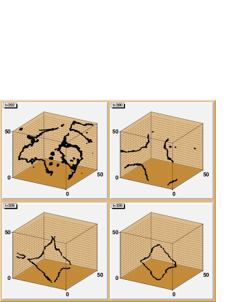
FIG. 5.: The process of string formation for ${\rm v}=3\times 10^{16}$ GeV and $\lambda=10^{-12}$.

Strings can be detected directly. For that purpose, we had plotted 3D coordinates of the grid points where $|\phi|$ is close to zero. A series of such images describing several different stages of this process is shown in Fig. 5. Strings are clearly seen, and we can observe the formation of one large loop.

At times $100<\tau<240$, while the zero mode was still oscillating, we had observed abundant formation and subsequent annihilation of string loops. Many strings appear when the oscillating zero mode $\langle\phi_{1}(t)\rangle$ passes through $\phi_{1}=0$. Then they disappear when $\langle\phi_{1}\rangle$ grows and appear when it becomes small again. Fig. 5, on the other hand, shows the behavior of strings after the phase transition, when the field $\phi_{1}$ is not capable of rolling over the top of the effective potential. At this stage the new strings are not produced, and the old ones move slowly, changing their position because of the string tension.

It is interesting that at time $\tau=280$ there is only one string loop in the integration box (upon account of the periodic boundary conditions), see Fig. 5. (A single spatial configuration, like this one, of course corresponds to a particular realization of random initial conditions.) This loop stays intact, up to small vibrations, for a long time, being in quasi-equilibrium. However, later on, different segments of the loop quickly approach each other and reconnect at $\tau=328$, forming another loop configuration at $\tau=330$. This final loop collapses almost to a point, bounces once, collapses again and disappears. This process of reconnection and final collapse confirms that loops are dynamical strings, not accidental lines in space.

To find the range of ${\rm v}$ for which strings are produced we had run simulations with different values of ${\rm v}$ in the interval from $4\times 10^{15}$ to $10^{17}$ GeV. In all these cases we observed formation of string loops. From cosmological perspective, however, the most interesting possibility would be formation of an infinite string. One can expect that, at least when ${\rm v}$ is large, the probability of formation of long strings is higher in the case when the moment of the symmetry breaking nearly coincides with the moment when $\langle\phi_{1}\rangle$ passes through zero. If that expectation is correct, the number of long strings should be a non-monotonic function of ${\rm v}$.

To verify this conjecture we plotted the string distribution at the time $\Delta\tau=10$ after the phase transition (which happens at different times) for ${\rm v}=3\times 10^{16}$ GeV, $5\times 10^{16}$ GeV, $6\times 10^{16}$ GeV, and $10^{17}$ GeV, for $\lambda=10^{-13}$, see Fig. 6. As we see, for ${\rm v}=5\times 10^{16}$ GeV and $10^{17}$ GeV all loops are short, whereas for ${\rm v}=3\times 10^{16}$ GeV and $6\times 10^{16}$ GeV there are many large loops. This indicates a possibility of formation of a network of infinite strings for ${\rm v}=3\times 10^{16}$ GeV and $6\times 10^{16}$ GeV.

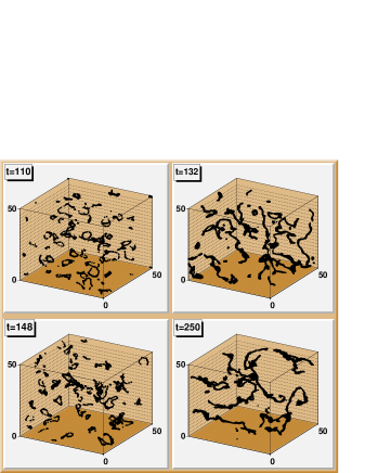
FIG. 6.: The string distribution at the time $\Delta\tau=10$ after the moment of the phase transition for ${\rm v}=10^{17}$ GeV, $6\times 10^{16}$ GeV, $5\times 10^{16}$ GeV, and $3\times 10^{16}$ GeV respectively. The plot for ${\rm v}=3\times 10^{16}$ GeV corresponds to a different realization of the initial conditions than Fig. 5.

Additional evidence for (or against) formation of infinite strings after preheating may be obtained if one uses lattices of a greater size. In particular, we performed simulations for ${\rm v}=3\times 10^{16}$ GeV in a larger box ($L=32\pi$), see Fig. 7. At the time shown in this figure, the physical size of the box is $L_{\rm phys}\sim(10^{2})m^{-1}$, where $m^{-1}\sim 1/\sqrt{\lambda}{\rm v}$ is the typical thickness of the string. In Fig. 7, we see two “infinite” strings and a large string loop. Note that on a lattice with periodic boundary conditions “infinite” strings can only be created in pairs, because the winding number for our initial conditions is zero.

Also, one may consider models where one may have independent reasons to expect production of infinite strings. For example, one may add to our model the term ${g^{2}\over 2}\phi^{2}\chi^{2}$ describing interaction of the inflaton field $\phi$ with the scalar field $\chi$ with the coupling constant $g^{2}\gg\lambda$. We have studied this model in Ref. [11] for the case of a one-component field $\phi$ and found a first-order phase transition. We expect that this result remains valid for the two-component field as well, because the main reason for the first order phase transition found in [11] was the strong interaction of the field $\phi$ with the field $\chi$ rather than the self-interaction of the field $\phi$. If this is indeed the case, then nonthermal fluctuations of the field $\chi$ will lead to symmetry restoration with respect to both of the fields $\phi_{1}$ and $\phi_{2}$. These two fields will be captured in the local minimum of the effective potential at $\phi=0$ until the moment of the first order phase transition. In this case, there will be strings formed by the usual Kibble mechanism, including infinite ones. We hope to return to the discussion of this model in a separate publication.

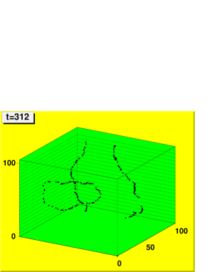
FIG. 7.: The string distribution for ${\rm v}=3\times 10^{16}$ GeV in a box of a larger size.

This work was supported in part by DOE grant DE-FG02-91ER40681 (Task B) (S.K. and I.T.), NSF grants PHY-9219345 (A.L.), PHY-9501458 (S.K. and I.T.), AST95-29-225 (L.K. and A.L.), and by the Alfred P. Sloan Foundation (S.K.).

REFERENCES

- [1] D.A. Kirzhnits, JETP Lett. 15, 529 (1972); D.A. Kirzhnits and A.D. Linde, Phys. Lett. 42B, 471 (1972); Sov. Phys. JETP 40, 628 (1974); Ann. Phys. 101, 195 (1976); S. Weinberg, Phys. Rev. D9, 3320 (1974); L. Dolan and R. Jackiw, Phys. Rev. D9, 3357 (1974).
- [2] L. A. Kofman, A. D. Linde, and A. A. Starobinsky, Phys. Rev. Lett. 73, 3195 (1994); L. A. Kofman, A. D. Linde, and A. A. Starobinsky, Phys. Rev.D 56, 3258 (1997), hep-ph/9704452.
- [3] L. Kofman, A. Linde, and A. A. Starobinsky, Phys. Rev. Lett. 76, 1011 (1996); I. I. Tkachev, Phys. Lett. B376, 35 (1996).
- [4] S.Yu. Khlebnikov and I.I. Tkachev, Phys. Rev. Lett. 77, 219 (1996), hep-ph/9603378.
- [5] S. Khlebnikov and I. Tkachev, Phys. Lett. B390, 80 (1997), hep-ph/9608458.
- [6] S. Khlebnikov and I. Tkachev, Phys. Rev. Lett. 79, 1607 (1997), hep-ph/9610477; S. Khlebnikov, hep-ph/9708313.
- [7] S. Khlebnikov and I. Tkachev, Phys. Rev. D56, 653 (1997), hep-ph/9701423.
- [8] T. Prokopec and T. G. Roos, Phys. Rev. D 55, 3768 (1997), hep-ph/9610400.
- [9] D. Boyanovsky, D. Cormier, H.J. de Vega, R. Holman, A. Singh, and M. Srednicki, Phys. Rev. D 56, 3929 (1997), hep-ph/9703327; S. Kasuya, M. Kawasaki, Phys. Rev. D 56, 7597 (1997), hep-ph/9703354.
- [10] I. I. Tkachev, S. Khlebnikov, L. Kofman, A. Linde, and A. A. Starobinsky, in preparation.
- [11] S. Khlebnikov, L. Kofman, A. Linde, and I. Tkachev, “First-order nonthermal phase transition after preheating,” hep-ph/9804425.
- [12] L. Kofman, a talk at COSMO97, Ambleside, 1997, hep-ph/9802221; L. Kofman, a talk at the 3rd RESECEU Symposium on Particle Cosmology, Tokyo 1997; A.D. Linde, talks at COSMO97, Ambleside, 1997, and at PASCOS98, Boston, 1998.
- [13] S. Kasuya, M. Kawasaki, “Topological defects formation after inflation on lattice simulations,” hep-ph/9804429.
- [14] D. Boyanovsky, H.J. de Vega, R. Holman, and J. Salgado, Phys. Rev. D 54, 7570 (1996); D.I. Kaiser, Phys. Rev. D 56, 706 (1997), hep-ph/9702244; P. B. Green, L. Kofman, A. D. Linde, and A. A. Starobinsky, Phys. Rev. D 56, 6175 (1997), hep-ph/9705347.