MC-TH-98/7

MAN/HEP/98/2

April 1998

Double Diffraction Dissociation at High $t$

B.E. Cox and J.R. Forshaw

Department of Physics and Astronomy,

University of Manchester,

Manchester, M13 9PL, England.

Diffractive scattering in the presence of a large momentum transfer is an ideal place to study the short distance rapidity gap producing mechanism. Previous studies (experimental and theoretical) in this area have focussed on gaps between jets and on high-$t$ vector meson production. We propose the measurement of double dissociation at high-$t$. We examine the numerous advantages to studying this more inclusive process and conclude that it is an ideal place to study short distance diffraction.

1 Introduction

In order to develop our understanding of diffractive processes, and in particular to understand them within the framework of QCD, it has been recognised that it is useful to focus in on a special class of diffractive phenomena: those that are driven by short distance physics. Large momentum transfer processes are especially good filters of short distance diffraction [1]. When we speak of large momentum transfer, we mean that the square of the four-momentum transferred across the associated rapidity gap, $-t$, is large. So, with this definition, inclusive small-$x$ deep inelastic scattering is not a large momentum transfer process (it is at $t=0$) whereas the ‘rapidity gaps between jets’ process suggested for study by Mueller & Tang [2] and measured at HERA [3] and the TEVATRON [4] colliders is. Quasi-elastic vector meson production at high $p_{t}$ is another example of a high-$t$ process which has been studied theoretically [5] and by experiment [6].

Let us begin by reviewing the current situation regarding the ‘gaps between jets’. Recall that one looks at the dependence of the production rate for events which contain a pair of jets and which have a rapidity gap between the jets, as a function of the gap size. The transverse momentum of the jets then makes sure that the gap producing mechanism is driven by small, i.e. $\lower 3.01385pt\hbox{$\;\stackrel{{\scriptstyle\textstyle<}}{{\sim}}\;$}1/p_{t}$, distances. Consequently, one can apply perturbative QCD and aim to really test the theory. On the theoretical side, the calculations have been performed within the leading logarithmic approximation (LLA) of BFKL [7] and predict an exponentially strong rise of the cross-section with increasing gap size. However, we note the LLA is not sufficient for a precise quantitative test of the theory [8]. In order to access the most interesting physics, it is necessary that data be collected at large rapidity gaps ($\lower 3.01385pt\hbox{$\;\stackrel{{\scriptstyle\textstyle>}}{{\sim}}\;$}4$). Unfortunately, the demand to observe a pair of high-$p_{t}$ jets within the detectors severely restricts the experimental reach. The TEVATRON experiments have collected data with gaps of up to 6 units between the jet centres, i.e. 4 units between the jet edges, whilst at HERA the experiments can only reach gaps of about 4 units between the jet centres. At HERA, this problem is somewhat circumvented by looking at high-$t$ vector meson production [5], but the rate is a low (although in time sufficient data will be collected) and one is limited to investigating the production of systems with fixed invariant mass. One also has the further complication that one needs to understand how the meson gets produced.

It is possible to avoid many of the above drawbacks by studying the more inclusive process where the incoming beam particles each dissociate, producing systems $X$ and $Y$ which are far apart in rapidity, in the presence of a large momentum transfer. The two processes discussed in the previous paragraph form subsets of this more inclusive measurement. Our subsequent studies will focus mainly on double dissociation at HERA, i.e. in photon-proton interactions. We expect similar results for double dissociation at the TEVATRON.

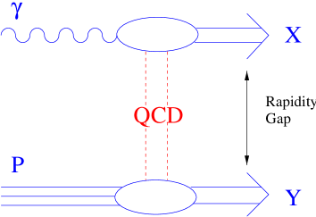
Figure 1: The double diffraction dissociation process.

Figure 1 shows the double dissociation process of our study. The photon dissociates to produce the system $X$, which travels in the backward direction whilst the proton dissociates to produce the system $Y$, which heads off in the forward direction. By not requiring to see a pair of jets in the detector we immediately open up the reach in rapidity by, as we shall shortly see, a very significant amount. We shall focus on photoproduction with a tagged electron (i.e. $Q^{2}\lower 3.01385pt\hbox{$\;\stackrel{{\scriptstyle\textstyle<}}{{\sim}}\;$}10^{-4}$ GeV²). An additional advantage is that the asymmetry of the beam energies at HERA ‘draws’ the system $X$ out of the backward beam hole making a measurement of its four-vector (and hence its invariant mass, $M_{X}$) possible. The entire kinematics of the event are determined by the measurement of the scattered electron (giving the four-vector of the photon) and the four-vector of the system $X$.

In order to select the events we do not propose that a gap cut be made. We follow the H1 procedure, wherein one uses the whole of the inclusive tagged photoproduction sample and, for each event, searches for the largest gap in the event [9]. This gap is then used to define the systems $X$ and $Y$, i.e. all particles backward of the gap go into system $X$ and all those forward of the gap go into system $Y$. Events with gaps are characterised by $M_{X},M_{Y}\ll W$ and so we choose to reduce the sample by insisting that $M_{Y}\leq M_{Y{\rm cut}}$. However we note that, given the momentum transfer four-vector, one can deduce $M_{Y}$ and hence that it is possible to measure the fully differential cross-section $d^{4}\sigma/(dWdt\ dM_{X}dM_{Y})$. We stress that we are not defining the sample in terms of a rapidity gap cut. This way of defining the sample has the very important advantage that it is easy to implement theoretically and is quite insensitive to hadronisation effects which define the edges of the systems $X$ and $Y$.

The remainder of the paper is organised as follows. We begin by presenting the relevant cross-section formulae. We then turn to Monte Carlo in order to examine issues relating to non-colour-singlet exchange and possible non-perturbative effects. We close by drawing our conclusions and alerting the reader to necessary future studies.

2 Kinematics and the double dissociation cross-section

Let $q_{\mu}$ be the four-momentum transfer. It has the following Sudakov decomposition:

$$q_{\mu}=\alpha P_{\mu}+\beta Q_{\mu}+q_{t,\mu}$$

where $P$ and $Q$ label the four-momenta of the incoming proton and photon. (We assume $P^{2}=Q^{2}=0$.) In the Regge limit, we have $t\equiv q^{2}\approx q_{t}^{2}$ and can write

$$M_{X}^{2} \approx t-\beta W^{2}$$

$$M_{Y}^{2} \approx t+\alpha W^{2}$$ (1)

where $W^{2}=(P+Q)^{2}=2P\cdot Q$.

Now, in the limit $-t\gg\Lambda_{{\rm QCD}}^{2}$ we can factorise the long distance physics into parton distribution functions and assume that the gap is produced by a single elastic parton-parton scattering, i.e. we can write

$$\frac{d\sigma(\gamma p\to XY)}{dx_{\gamma}dx_{h}dt}=F_{\gamma}(x_{\gamma},-t)F_{p}(x_{h},-t)\frac{d\hat{\sigma}(qq\to qq)}{dt}$$ (2)

where $F_{i}(x,\mu^{2})=\frac{9}{4}g_{i}(x,\mu^{2})+\Sigma_{i}(x,\mu^{2})$ is a colour weighted sum over gluon and quark parton density functions for beam particle $i$. The fraction of the beam momentum carried by the struck parton is $x$ and $\mu$ is the factorisation scale. The perturbative QCD dynamics lies in the cross-section for elastically scattering a pair of quarks: $d\hat{\sigma}(qq\to qq)/dt$. In the leading logarithm approximation, this is given by exchanging a pair of interacting reggeised gluons [7]. In the asymptotic limit $x_{\gamma}x_{h}W^{2}\gg-t$ the cross-section can be computed analytically [2]:

$$\frac{d\hat{\sigma}(qq\to qq)}{dt}=(\alpha_{s}C_{F})^{4}\frac{2\pi^{3}}{t^{2}}\frac{e^{2\omega_{0}Y}}{(7\alpha_{s}N_{c}\zeta(3)Y)^{3}}$$ (3)

where

$$Y=\ln\left(\frac{x_{\gamma}x_{h}W^{2}}{-t}\right)$$

and

$$\omega_{0}=N_{c}\ 4\ln 2\ \frac{\alpha_{s}}{\pi}.$$

This result has already been coded into HERWIG [10], as has the exact leading logarithm expression [11].

An alternative model for the gap producing mechanism is to assume that two massive gluons are exchanged, in which case

$$\frac{d\hat{\sigma}(qq\to qq)}{dt}=\frac{\pi}{16t^{2}}\alpha_{s}^{4}\frac{1}{\Delta^{2}}\ln^{2}\frac{\Delta+1}{\Delta-1},$$ (4)

where

$$\Delta=(1-4M^{2}/t)^{1/2}$$ (5)

and $M$ is the gluon mass. We have also incorporated this process into HERWIG.

The incoming partons are collinear with the beam particles whilst, after the scatter, they carry transverse momentum $\sqrt{(-t)}$. These partons are the seeds of the jets which are produced in the gaps between jets measurement. Putting these outgoing partons on shell gives

$$x_{\gamma}=\frac{-t}{-\beta W^{2}} = \frac{-t}{\tilde{M}_{X}^{2}}$$

$$x_{h}=\frac{-t}{\alpha W^{2}} = \frac{-t}{\tilde{M}_{Y}^{2}}.$$ (6)

We have defined $\tilde{M}_{X}^{2}\equiv M_{X}^{2}-t$ and $\tilde{M}_{Y}^{2}=M_{Y}^{2}-t$. These kinematic relations between the parton momentum fractions and the physical observables allow us to write

$$\tilde{M}_{X}^{2}\tilde{M}_{Y}^{2}\frac{d\sigma}{\tilde{M}_{X}^{2}\tilde{M}_{Y}^{2}}=x_{\gamma}x_{h}\frac{d\sigma}{dx_{\gamma}dx_{h}}.$$

For the purposes of this paper, we will assume that $M_{Y}$ is confined to be smaller than some value. Recall that the Regge limit demands that $W\gg M_{X},M_{Y}$ and hence that there be a rapidity gap between the systems $X$ and $Y$. In particular we take $M_{Y}<10$ GeV. Although it would be very interesting to look at variations with $M_{Y}$.

We shall also use the popular notation

$$x_{{}_{\rm I\!P}}\equiv-\beta=\frac{\tilde{M}_{X}^{2}}{W^{2}}.$$

In which case

$$\frac{d\sigma(\gamma p\to XY)}{dx_{{}_{\rm I\!P}}dt}=\frac{1}{t^{2}}\int dM_{Y}^{2}\ (x_{\gamma}x_{h}W)^{2}F_{\gamma}(x_{\gamma},-t)F_{p}(x_{h},-t)\frac{d\hat{\sigma}(qq\to qq)}{dt}.$$ (7)

Sitting at fixed $M_{X}^{2}$ and $t$ the $x_{{}_{\rm I\!P}}$ dependence is determined completely by the hard partonic scattering. For example, if

$$\frac{d\hat{\sigma}(qq\to qq)}{dt}\sim e^{2\omega_{0}Y}$$ (8)

then

$$\frac{d\sigma(\gamma p\to XY)}{dx_{{}_{\rm I\!P}}dt}\sim\left(\frac{1}{x_{{}_{\rm I\!P}}}\right)^{2\omega_{0}+1}.$$ (9)

Alternatively, one can look at the $x_{{}_{\rm I\!P}}$ dependence at fixed $W$ and $t$. In which case the $x_{{}_{\rm I\!P}}$ dependence is dependent upon the photon parton densities, i.e. if the hard scatter is given by (8) then it follows that

$$\frac{d\sigma(\gamma p\to XY)}{dx_{{}_{\rm I\!P}}dt}\sim\left(\frac{1}{x_{{}_{\rm I\!P}}}\right)^{2\omega_{0}+2}F_{\gamma}(x_{\gamma},-t)$$ (10)

where $x_{\gamma}=-t/(x_{{}_{\rm I\!P}}W^{2})$.

In Fig.2 we compare the massive gluon and BFKL calculations of the $\gamma p$ cross-section (all the cross-sections we show will be for $\gamma p$ interactions). For the massive gluon calculation, we chose a gluon mass of 800 MeV. Decreasing the mass causes the cross-section to rise (it diverges at zero mass) but does not affect the shape of the $x_{{}_{\rm I\!P}}$ distribution; it remains significantly flatter than the BFKL calculation. The cross-sections are shown for two different values of the parameter $\alpha_{s}$. Increasing $\alpha_{s}$ steepens the BFKL distribution (since $\omega_{0}\sim\alpha_{s}$) but only affects the normalisation of the massive gluon distribution.

For all our plots we take $W=250$ GeV, $-t>4$ GeV² and $M_{Y}<10$ GeV. Unless otherwise stated, all our results are derived using the BFKL calculation with $\alpha_{s}=0.23$ and using the GRV-G HO parton distribution functions of the photon [12] and the GRV 94 HO DIS proton parton density functions [13] as implemented in PDFLIB [14]. We choose to show plots at fixed $W$ (rather than fixed $M_{X}$ say) since this is the more natural scenario for a first measurement.

In Fig.3 we show the effect of varying the photon parton density functions [12, 15, 16, 17]. We note that the primary effect of varying the photon parton density functions is to shift the normalisation. In fact, for the BFKL calculation, the $x_{{}_{\rm I\!P}}$ behaviour is quite close to $\sim(1/x_{{}_{\rm I\!P}})^{2\omega_{0}}$ independent of the photon parton density function (compare this with the expectation of (10)). Note that changing the proton parton density functions does not affect the shape of the $x_{{}_{\rm I\!P}}$ distribution, since $x_{h}$ depends only upon $t$ and $M_{Y}$.

3 Monte Carlo simulation

Since the BFKL and massive gluon calculations have been implemented into HERWIG, we are able to perform a simulation to hadron level which includes the background expected from fluctuations in non-colour-singlet exchange photoproduction processes. HERWIG is used to generate 2.5 pb^-1 of $ep$ data. For each event with a tagged electron, the largest rapidity gap in the event is sought and this is used to define the systems $X$ and $Y$. The kinematic cuts described in the previous section are then applied.

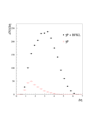
Figure 4: Distribution of events in rapidity.

In Fig.4 we show the distribution of our events as a function of the rapidity gap (only events which have $10^{-3}<x_{{}_{\rm I\!P}}<10^{-2}$ are included). Those events which originate from non-colour-singlet exchange processes are also shown and can be seen to constitute a small fraction of the total. This effective depletion of the non-colour-singlet exchange contribution arises directly as a consequence of our insisting that $M_{Y}<10$ GeV and $10^{-3}<x_{{}_{\rm I\!P}}<10^{-2}$, i.e. that $M_{X},M_{Y}\ll W$. In particular, no rapidity gap cut is needed to select rapidity gap events.

Since we are not requiring to see system $Y$ in the detector, it is now possible to select events with very large gaps. Also, since we are not requiring to see jets, many more events enter the sample than entered the gaps between jets measurement (this arises primarily because most events lie at the lowest values of $-t$). We wish to emphasise the magnitude of the gain in both statistics and reach in rapidity. In particular, we note that the HERA gaps between jets data populate the $\Delta\eta<2$ region and that, even in this restricted region, they constitute only a small fraction of the total number of events.

In Fig.5 we show the $x_{{}_{\rm I\!P}}$ distribution at fixed $W$. The errors are typical of the statistical errors to be expected from analysis of data already collected at HERA. The small contribution from non-colour-singlet exchange processes is included. This is shown separately in Fig.6 and, as expected, it falls away exponentially as $x_{{}_{\rm I\!P}}$ falls.

We expect that the data will be suitable for making very precise statements regarding the dependence of the gap production mechanism upon the gap size.

In Fig.7 we compare the theoretical calculation with the output from HERWIG. The open circles correspond to the cross-section obtained when $t$ is constructed at the level of the hard scatter, i.e. it is the $t$ of the hard BFKL subprocess. Of course this value of $t$ should be unique and equal to the value extracted by summing the four-momenta of all outgoing hadrons in system $X$ and subtracting from the four-momenta of the incoming photon. The solid circles in Fig.7 show the effect of reconstructing $t$ at the hadron level and clearly there is a significant shift relative to the hard scatter points (which agree well with the theoretical calculation). The squares denote the cross-section obtained by computing $t$ after parton showering but before hadronisation.

The fact that the reconstructed $t$ values are not all the same is clearly demonstrated in Fig.8. The number of events is plotted as a function of the difference in $t$ between the value extracted after parton showering, $t_{ps}$, and the value obtained from the hard scatter, $t_{hs}$. Note that there is no shift in $t$ for those events we have labelled ‘valence’. These are events in which the parton entering the hard scatter from the proton is either an up or a down quark and from the photon is not a gluon. All other events are in the ‘non-valence’ sample and it is here we see the systematic shift to larger values of $-t$, i.e. $-t_{ps}>-t_{hs}$. This shift is a consequence of the way HERWIG develops the final state from the seed partons in the hard scatter. In particular, since HERWIG generates the complete final state it necessarily has some model for the photon and proton remnants. For the proton, it will always evolve backwards from the hard scatter to a valence quark, whereas for the photon evolution terminates with a quark–anti-quark pair. Hence, in the ‘non-valence’ sample at least one parton must be emitted off an incoming parton. This is the source of the shift in $t$.

A shift to large $-t$ has the immediate consequence of systematically shifting the $x_{{}_{\rm I\!P}}$ distribution to the right, as is clearly seen in Fig.7. This is easy to see since $x_{{}_{\rm I\!P}}=(M_{X}^{2}-t)/W^{2}$, so events which are generated with some $t_{hs}$ are reconstructed, after parton showering, to have a larger $-t$ and hence larger $x_{{}_{\rm I\!P}}$. In essence therefore, the difference between the theory and hadron level results can be attributed to non-perturbative effects. The primary feature of the effect is to systematically shift the $x_{{}_{\rm I\!P}}$ distribution without significantly affecting its shape.

4 Outlook

We have proposed a new way of studying short distance diffraction. We believe this measurement can be made by the HERA experimentalists. Things may not be so simple at the TEVATRON, where one does not have the asymmetric beam energies to boost one of the diffracted systems into the detectors. Our proposal optimises the statistics, allows a wide reach in rapidity, has very small hadronisation corrections and very little background. It is also easy to extract a cross-section for comparison with theory.

We have not discussed the issue of gap survival. This is a topic for further discussion. For now let us point out that, should the gap survival probability decrease with increasing $W$ but be approximately constant at fixed $W$ (this possibility is anticipated since the probability for secondary partonic interactions, which would destroy the gap, increases as the number density of partons increases and since the parton density is largest at small $x$, i.e. high $W$ [18]) then the $x_{{}_{\rm I\!P}}$ at fixed $M_{X}$ and $x_{{}_{\rm I\!P}}$ at fixed $W$ distributions would provide complementary information.

Figure 2: Comparison of the BFKL (solid and dashed lines) and massive gluon (dotted and dashed-dotted lines) predictions.

Figure 3: Effect of varying the photon parton density functions.

Figure 5: The $x_{{}_{\rm I\!P}}$ distribution at fixed $W$.

Figure 6: The $x_{{}_{\rm I\!P}}$ distribution of the background due to non-colour-singlet exchange.

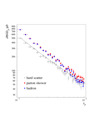
Figure 7: Comparison of theory (solid line) with the Monte Carlo output from HERWIG.

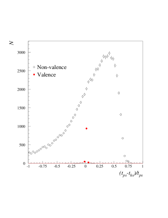
Figure 8: Deviation of the reconstructed $t$ from the true value.

References

- [1] J.R.Forshaw and P.J.Sutton, Eur.Phys.J. C1 (1998) 285.
- [2] A.H.Mueller and W.-K.Tang, Phys.Lett. B284, (1992) 123.
- [3] ZEUS Collaboration: M.Derrick et al., Phys.Lett. B369 (1996) 55; H1 Collaboration: “Rapidity Gaps Between Jets in Photoproduction at HERA” contribution to The International Europhysics Conference on High Energy Physics, August 1997, Jerusalem, Israel.
- [4] CDF Collaboration: F.Abe et al., Phys.Rev.Lett. 74 (1995) 855; D0 Collaboration: S.Abachi et al., Phys.Rev.Lett. 76 (1996) 734.
- [5] I.F.Ginzberg, S.L.Panfil and V.G.Serbo, Nucl.Phys. B284 (1987) 685; J.R.Forshaw and M.G.Ryskin, Z.Phys. C68 (1995) 137; J.Bartels, J.R.Forshaw, M.Wüsthoff and H.Lotter, Phys.Lett. B375 (1996) 301; D.Yu.Ivanov, Phys.Rev. D53 (1996) 3564; I.F.Ginzburg and D.Yu.Ivanov, Phys.Rev. D54 (1996) 5523.
- [6] H1 Collaboration: “Production of Mesons with large at HERA” contribution to The International Europhysics Conference on High Energy Physics, August 1997, Jerusalem, Israel; ZEUS Collaboration: “Study of Vector Meson Production at Large at HERA” contribution to The International Europhysics Conference on High Energy Physics, August 1997, Jerusalem, Israel.
- [7] E.A.Kuraev, L.N.Lipatov and V.S.Fadin, Sov.Phys.JETP 45 (1977) 199; Ya.Ya.Balitsky and L.N.Lipatov, Sov.J.Nucl.Phys 28 (1978) 822; L.N.Lipatov, Sov.Phys.JETP 63 (1986) 904.
- [8] L.N.Lipatov and V.S.Fadin, Sov.J.Nucl.Phys. 50 (1989) 712; JETP Lett. 89 (1989) 352; V.S.Fadin and R.Fiore, Phys.Lett. B294 (192) 286; V.S.Fadin and L.N.Lipatov, Nucl.Phys. B406 (1993) 259; B477 (1996) 767; hep-ph/9802290; V.S.Fadin, R.Fiore and A.Quartarolo, Phys.Rev. D50 (1994) 2265; D50 (1994) 5893; D53 (1996) 2729; V.S.Fadin, R.Fiore and M.I.Kotsky, Phys.Lett. B387 (1996) 593; Phys.Lett. B359 (1995) 181; V.S.Fadin, M.I.Kotsky and L.N.Lipatov, hep-ph/9704267; V.S.Fadin et al., hep-ph/9711427; G.Camici and M.Ciafaloni, Phys.Lett. B386 (1996) 341; Nucl.Phys. B496 (1997) 305; M.Ciafaloni and G.Camici, Phys.Lett. B412 (1997) 396 and erratum; hep-ph/9803389.
- [9] H1 Collaboration: C.Adloff et al., Z.Phys. C74 (1997) 221.
- [10] G.Marchesini et al., Comp.Phys.Comm. 67 (1992) 465.
- [11] M.E.Hayes, Bristol University, PhD Thesis (1998).
- [12] M.Glück, E.Reya and A.Vogt, Phys.Rev. D45 (1992) 3986.
- [13] M.Glück, E.Reya and A.Vogt, Z.Phys. C67 (1995) 433.
- [14] H.Plothow-Besch: PDFLIB Users Manual, W5051 PDFLIB, 1997.07.02, CERN-PPE; Int.J.Mod.Phys. A10 (1995) 2901.
- [15] H.Abramowicz, K.Charchula and A.Levy, Phys.Lett. B269 (1991) 458.
- [16] P.Aurenche, M.Fontannaz and J.Ph.Guillet, Z.Phys. C64 (1994) 621.
- [17] L.E.Gordon and J.K.Storrow, Nucl.Phys. B489 (1997) 405.
- [18] J.M.Butterworth, J.R.Forshaw and M.H.Seymour, Z.Phys. C72 (1996) 637.