QCD Calculations by Numerical Integration

Abstract

Calculations of observables in Quantum Chromodynamics are typically performed using a method that combines numerical integrations over the momenta of final state particles with analytical integrations over the momenta of virtual particles. I discuss a method for performing all of the integrations numerically.

This Letter concerns a method for performing perturbative calculations in Quantum Chromodynamics (QCD) and other quantum field theories. Specifically, I am concerned with cross sections and other QCD observables in which one measures something about the hadronic final state. Here one cannot use the special techniques that apply to inclusive quantities like the structure functions in deeply inelastic lepton scattering. The general class of calculations of interest in this Letter includes jet cross sections in hadron-hadron and lepton-hadron scattering and in $e^{+}e^{-}\to{\it hadrons}$. There have been many calculations of this kind carried out at next-to-leading order in perturbation theory, resulting in an impressive confrontation between theory and experiment and in an accumulation of evidence supporting QCD as the correct theory of the strong interactions [1]. These calculations are based on a method introduced by Ellis, Ross, and Terrano [2] in the context of $e^{+}e^{-}\to{\it hadrons}$. Stated in the simplest terms, the Ellis-Ross-Terrano method is to do some integrations over momenta $\vec{p}_{i}$ analytically, others numerically. I shall argue that it is possible instead to do all of these integrations numerically. Furthermore, I shall argue that performing all of the integrations numerically has some advantages, principally in the flexibility that it allows.

In this Letter, I address only the process $e^{+}e^{-}\to{\it hadrons}$. Thus I do not address the issue of factorization that is associated with initial state hadrons. I discuss three-jet-like infrared safe observables at next-to-leading order, that is order $\alpha_{s}^{2}$. Examples of such observables include the thrust distribution, the fraction of events that have three jets, and the energy-energy correlation function.

Let us begin with a precise statement of the problem. The order $\alpha_{s}^{2}$ contribution to the observable being calculated has the form

$$\sigma^{[2]} = {1\over 2!}\int d\vec{k}_{1}d\vec{k}_{2}\ {d\sigma^{[2]}_{2}\over d\vec{k}_{1}d\vec{k}_{2}}\ {\cal S}_{2}(\vec{k}_{1},\vec{k}_{2})$$ (3)

$$+{1\over 3!}\int d\vec{k}_{1}d\vec{k}_{2}d\vec{k}_{3}\ {d\sigma^{[2]}_{3}\over d\vec{k}_{1}d\vec{k}_{2}d\vec{k}_{3}}\ {\cal S}_{3}(\vec{k}_{1},\vec{k}_{2},\vec{k}_{3})$$

$$+{1\over 4!}\int d\vec{k}_{1}d\vec{k}_{2}d\vec{k}_{3}d\vec{k}_{4}\ {d\sigma^{[2]}_{4}\over d\vec{k}_{1}d\vec{k}_{2}d\vec{k}_{3}d\vec{k}_{4}}\ {\cal S}_{4}(\vec{k}_{1},\vec{k}_{2},\vec{k}_{3},\vec{k}_{4}).$$

Here the $d\sigma^{[2]}_{n}$ are the order $\alpha_{s}^{2}$ contributions to the parton level cross section, calculated with zero quark masses. Each contains momentum and energy conserving delta functions. The $d\sigma^{[2]}_{n}$ include ultraviolet renormalization in the  MS  scheme. The functions $\cal S$ describe the measurable quantity to be calculated. We wish to calculate a “three-jet” quantity. That is, ${\cal S}_{2}=0$. The normalization is such that ${\cal S}_{n}=1$ for $n=2,3,4$ would give the order $\alpha_{s}^{2}$ perturbative contribution the the total cross section. There are, of course, infrared divergences associated with Eq. (3). For now, we may simply suppose that an infrared cutoff has been supplied.

The measurement, as specified by the functions ${\cal S}_{n}$, is to be infrared safe, as described in Ref. [3]: the ${\cal S}_{n}$ are smooth functions of the parton momenta and

$${\cal S}_{n+1}(\vec{k}_{1},\dots,\lambda\vec{k}_{n},(1-\lambda)\vec{k}_{n})={\cal S}_{n}(\vec{k}_{1},\dots,\vec{k}_{n})$$ (4)

for $0\leq\lambda<1$. That is, collinear splittings and soft particles do not affect the measurement.

It is convenient to calculate a quantity that is dimensionless. Let the functions ${\cal S}_{n}$ be dimensionless and eliminate the remaining dimensionality in the problem by dividing by $\sigma_{0}$, the total $e^{+}e^{-}$ cross section at the Born level. Let us also remove the factor of $(\alpha_{s}/\pi)^{2}$. Thus, we calculate

$${\cal I}={\sigma^{[2]}\over\sigma_{0}\ (\alpha_{s}/\pi)^{2}}.$$ (5)

We note that ${\cal I}$ is a function of the c.m. energy $\sqrt{s}$ and the $\overline{\rm MS}$ renormalization scale $\mu$. We will choose $\mu$ to be proportional to $\sqrt{s}$: $\mu=A_{UV}\sqrt{s}$. Then ${\cal I}$ depends on $A_{UV}$. But, because it is dimensionless, it is independent of $\sqrt{s}$. This allows us to write

$${\cal I}=\int_{0}^{\infty}d\sqrt{s}\ h(\sqrt{s})\ {\cal I}(A_{UV},\sqrt{s}),$$ (6)

where $h$ is any function with

$$\int_{0}^{\infty}d\sqrt{s}\ h(\sqrt{s})=1.$$ (7)

The integration over $\sqrt{s}$ eliminates the energy conserving delta function in $\cal I$. The physical meaning is that, by smearing in the energy $\sqrt{s}$, we force the time variables in the two current operators that create the hadronic state to be within $1/\sqrt{s}$ of each other. Thus we have a truly short distance problem.

I now describe how one would calculate $\cal I$ using the Ellis-Ross-Terrano method. Each partonic cross section in Eq. (3) can be expressed as an amplitude times a complex conjugate amplitude. One must calculate the amplitudes in $4-2\epsilon$ dimensions. (In the case of the process $e^{+}e^{-}\to{\it hadrons}$, this calculation was performed by Ellis, Ross, and Terrano [2].) For tree diagrams, the calculation is straightforward. For loop diagrams, this involves an integration, which is performed analytically. The integrals are divergent in four dimensions, so one obtains divergent terms proportional to $1/\epsilon^{2}$ and $1/\epsilon$ in addition to terms that are finite as $\epsilon\to 0$. Having the amplitudes and complex conjugate amplitudes, one must now multiply by the functions ${\cal S}_{n}$ and integrate over the final state parton momenta. These integrations are too complicated to perform analytically, so one must use numerical methods. Unfortunately, the integrals are divergent at $\epsilon=0$. Thus one must split the integrals into two parts. One part can be divergent at $\epsilon=0$ but must be simple enough to calculate analytically. The other part can be complicated, but must be convergent at $\epsilon=0$. One calculates the simple, divergent part and cancels the $1/\epsilon^{2}$ and $1/\epsilon$ pole terms against the pole terms coming from the virtual loop diagrams. This leaves the complicated, convergent integration to be performed numerically.

This method is a little bit cumbersome, but it works and has been enormously successful. However it has proven to be difficult to apply the method in the case of two virtual loops. Even with one virtual loop, the method is not very flexible. Any modification of the integrand requires one to recalculate the amplitudes, and the modification must be simple enough that one can calculate the amplitudes in closed form.

Let us, therefore, inquire whether there is any other way that one might perform such a calculation. We note that the quantity $\cal I$ can be expressed in terms of cut Feynman diagrams, as in Fig. 1. The part of the diagram to the left of the cut is a term in the amplitude. The part to the right of the cut is a term in the complex conjugate amplitude. The dots where the parton lines cross the cut are intended to represent the function ${\cal S}_{n}(\vec{k}_{1},\dots,\vec{k}_{n})$. Each diagram is a three loop diagram, so we have integrations over loop momenta $\ell_{1}^{\mu}$, $\ell_{2}^{\mu}$ and $\ell_{3}^{\mu}$.

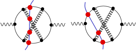
FIG. 1.: Two cuts of one of the Feynman diagrams that contribute to $e^{+}e^{-}\to{\it hadrons}$.

We first perform the energy integrations. For the graphs in which four parton lines cross the cut, there are four mass-shell delta functions $\delta(k_{J}^{2})$. These delta functions eliminate the three energy integrals over $\ell_{1}^{0}$, $\ell_{2}^{0}$, and $\ell_{3}^{0}$ as well as the integral (6) over $\sqrt{s}$. For the graphs in which three parton lines cross the cut, we can eliminate the integration over $\sqrt{s}$ and two of the $\ell_{J}^{0}$ integrals. One integral over the energy $E$ in the virtual loop remains. The integrand contains a product of factors

$${i\over E-Q_{J}^{0}-\omega_{J}+i\epsilon}\,{1\over E-Q_{J}^{0}+\omega_{J}-i\epsilon},$$ (8)

where $E-Q^{0}_{J}$ is the energy carried by the $J$th propagator around the loop and $\omega_{J}$ is the absolute value of the momentum carried on that propagator. We perform the integration by closing the integration contour in the lower half $E$ plane. This leads to $n$ terms for a virtual $n$ point subgraph. In the $J$th term, the propagator energy $E-Q^{0}_{J}$ is set equal to the corresponding $\omega_{J}$ and there is a factor $1/(2\omega_{J})$. Note that the entire process of performing the energy integrals amounts to some simple algebraic substitutions.

Let us denote the contribution to $\cal I$ from the cut $C$ of graph $G$ by ${\cal I}(G,C)$. This contribution has the form

$${\cal I}(G,C)=\int d^{3}\vec{\ell}_{1}\,d^{3}\vec{\ell}_{2}\,d^{3}\vec{\ell}_{3}\ g(G,C;\ell),$$ (9)

where $\ell$ denotes the set of loop momenta $\{\vec{\ell}_{1},\vec{\ell}_{2},\vec{\ell}_{3}\}$. The functions $g$ have some singularities, called pinch singularities, that cannot be avoided by deforming the integration contour and some non-pinch singularities that can be avoided by a contour deformation. A detailed analysis, which I sketch below, has been given by Sterman [4].

The pinch singularities occur when one parton branches into two partons with collinear momenta or when one parton momentum goes to zero. These singularities can lead to logarithmic divergences in the corresponding integral. (As pointed out in [4], the $q^{\mu}q^{\nu}$ terms in gluon self-energy subgraphs lead to quadratic divergences. I will discuss these terms shortly.) If we were to calculate the total cross section by using measurement functions ${\cal S}_{n}=1$ in $g$, then the singularities would cancel [4] between the functions $g$ associated with the various cuts $C$ of the same graph $G$. The underlying reason is unitarity. Now in our case of measured shape variables, the values of ${\cal S}_{n}$ corresponding to different cuts $C$ are different. This would ruin the cancellation, except that just at the collinear or soft points the functions ${\cal S}_{n}$ match. Thus the singularities present in the individual $g(G,C;\ell)$ cancel in the sum, $\sum_{C}g(G,C;\ell)$. To be precise, the cancellation reduces the strength of the singularity from a strength sufficient to give a logarithmically divergent integral to one that gives a convergent integral.

The function $g$ also has singularities that can be avoided by deforming the integration contours, the non-pinch singularities. These can be characterized rather simply in the present case of a single virtual loop. Let $\vec{\ell}$ be the a loop momentum that flows around this virtual loop. We may choose $\vec{\ell}$ so that it is the momentum carried by one of the loop propagators and so that a momentum $\vec{Q}$ flows out of the loop and into the final state between the propagator in question and another propagator further along the loop. This second propagator carries momentum $\vec{\ell}-\vec{Q}$. A positive energy $Q^{0}$ also flows out of the loop and into the final state. Since $(Q^{0},\vec{Q})$ is the four-momentum of a group of final state particles, we have $Q^{0}\geq|\vec{Q}|$. Then there is a singularity when $|\vec{\ell}|+|\vec{\ell}-\vec{Q}|=Q^{0}$. In the case $Q^{0}=|\vec{Q}|$, this is a collinear singularity, and will cancel between cuts. In the case $Q^{0}>|\vec{Q}|$, the singular surface is an ellipsoid. The singularity does not cancel, but the Feynman rules provide an $i\epsilon$ prescription that tells us that we should deform the $\vec{\ell}$ integration contour into the complex $\vec{\ell}$ plane so as to avoid the singularity. Here deforming the contour means replacing $\vec{\ell}$ by a complex vector $\vec{\ell}+i\vec{\kappa}$. Then one simply chooses the imaginary part, $\vec{\kappa}$, of the loop momentum as a function of the real part, $\vec{\ell}$, and supplies an appropriate jacobian $\cal J$. Since the momentum $\vec{\ell}$ that flows around the virtual loop in question is, in general, a linear combination of the three loop momenta $\vec{\ell}_{j}$, one should write the general relation as $\vec{\ell}_{j}\to\vec{\ell}_{j}+i\vec{\kappa}_{j}$, or, in a abbreviated notation, $\ell\to\ell+i\kappa$. Then

$${\cal I}(G,C)=\int d^{3}\vec{\ell}_{1}\,d^{3}\vec{\ell}_{2}\,d^{3}\vec{\ell}_{3}\ {\cal J}(G,C;\ell)\ g(G,C;\ell+i\kappa(G,C;\ell)).$$ (10)

Note that the contour deformation is more than just a mathematical trick. The analyticity that allows it is a consequence of the causality property of the field theory.

Now, there is a simple argument that the pinch singularities cancel between different cuts $C$ of the same graph $G$. There is another simple argument that the non-pinch singularities are not a problem because one can deform the integration contours so as to avoid them. If one is being careful in the proof, one notes that the deformations required to escape the non-pinch singularities are different for each cut $C$. (The deformations for different cuts must be different if one wants the momenta of final state particles to be real.) On the other hand, the cancellation of pinch singularities requires that the contours for different cuts $C$ be the same as one approaches the pinch singularities. That is, the set of vectors $\{\vec{\kappa}_{1},\vec{\kappa}_{2},\vec{\kappa}_{3}\}$ that define the deformation associated with a cut $C$ must to go to zero as $\{\vec{\ell}_{1},\vec{\ell}_{2},\vec{\ell}_{3}\}$ approaches a pinch singular surface.

This sort of consideration of how to prove that $\cal I$ is finite instructs us how to actually calculate $\cal I$. With the contours appropriately chosen, the integral

$${\cal I}(G)=\int d^{3}\vec{\ell}_{1}\,d^{3}\vec{\ell}_{2}\,d^{3}\vec{\ell}_{3}\ \sum_{C}\,{\cal J}(G,C;\ell)\ g(G,C;\ell+i\kappa(G,C;\ell))$$ (11)

is finite. One can simply compute it by Monte Carlo integration. Note the significance of putting the summation over cuts inside the integral. When we sum over cuts for a given point in the space of loop momenta, the soft and collinear divergences cancel because the cancellation is built into the Feynman rules. If we were to put the sum over cuts outside the integration, as in the Ellis-Ross-Terrano method, then the individual integrals would be divergent. The calculation would thereby be rendered more difficult.

Eq. (11) represents the main point of this Letter. It is perhaps useful to point out that one must remove from the integration tiny regions near the collinear and soft singular points, since otherwise roundoff errors would spoil the cancellation of the individual contributions. I leave for later, more specialized, papers the details of how one can choose a specific contour deformation so that the theoretical cancellation is realized in practice. I also skip a discussion of how one can choose the density of integration points so as to perform the numerical integration by the Monte Carlo method. There are, however, two points of principle that I discuss below, since they are not analyzed in Ref. [4]: renormalization and the special treatment required for self-energy subgraphs.

Renormalization is conventionally accomplished by performing loop integrations in $4-2\epsilon$ space-time dimensions and subtracting the resulting pole term, $c/\epsilon$. Clearly that is not appropriate in a numerical integration. However, one can subtract instead an integral in 4 space-time dimensions such that, in the region of large loop momenta, the integrand of the subtraction term matches the integrand of the subgraph in question. The integrand of the subtraction term can depend on a mass parameter $\mu$ in such a way that the subtraction term has no infrared singularities. Then, one can easily arrange that this ad hoc subtraction has exactly the same effect as  MS  subtraction with scale parameter $\mu$.

Self-energy subgraphs require a special treatment. Consider a quark self-energy subgraph $-i\Sigma$ with one adjoining virtual propagator and one adjoining cut propagator. This combination really represents a field strength renormalization for the quark field, and is interpreted as

$${1\over 2}\left[{\hbox to0.0pt{/\hss}q\over q^{2}}\,\Sigma(q)\,\hbox to0.0pt{/\hss}q\right]_{q^{2}=0}\,2\pi\delta(q^{2}).$$ (12)

In order to take the $q^{2}\to 0$ limit here while at the same time maintaining the cancellation of collinear divergences, we write

$${\hbox to0.0pt{/\hss}q\,\Sigma(q)\,\hbox to0.0pt{/\hss}q\over q^{2}}=-{g^{2}\over(2\pi)^{3}}\,C_{F}\int d^{3}\vec{\ell}\ {q^{0}|\vec{k}_{+}|\gamma^{0}-(|\vec{k}_{+}|+|\vec{k}_{-}|)\vec{k}_{+}\cdot\vec{\gamma}\over|\vec{k}_{+}||\vec{k}_{-}|\left[(|\vec{k}_{+}|+|\vec{k}_{-}|)^{2}-(q^{0})^{2}\right]},$$ (13)

where $\vec{k}_{\pm}={1\over 2}\vec{q}\pm\vec{\ell}$. This expression is obtained by writing the left-hand side as a dispersive integral with the cut self-energy graph appearing as the discontinuity. When the virtual self-energy is written in this form, the $q^{2}\to 0$ limit is smooth and, in addition, the cancellation between real and virtual graphs in the collinear limit $\vec{\ell}\propto\vec{q}$ is manifest. It should be noted that the integral in Eq. (13) is ultraviolet divergent and requires renormalization, which can be performed with an ad hoc subtraction as described above.

One may expect that the representation of virtual propagator corrections in terms of the cut propagator will prove to be convenient in future modifications of the method described in this Letter. One may want to make modifications to the gluon propagator, in particular, in order to implement a running strong coupling and to insert models for the long distance propagation of gluons. In addition, one may want to modify propagators so that partons can enter the final state with $q^{2}>0$ so as to mesh an order $\alpha_{s}^{2}$ perturbative calculation with a parton shower Monte Carlo program.

Consider, finally, the one loop gluon self-energy subgraph, $\pi^{\mu\nu}(q)$. The term in $\pi^{\mu\nu}(q)$ proportional to $q^{\mu}q^{\nu}$ contributes quadratic infrared divergences [4]. This problem can be addressed by replacing $\pi^{\mu\nu}$ by $P^{\mu}_{\alpha}\pi^{\alpha\beta}P_{\beta}^{\nu}$, where $P^{\mu}_{\alpha}=g^{\mu}_{\alpha}-{q^{\mu}\tilde{q}_{\alpha}/\tilde{q}^{2}},$ with $\tilde{q}=(0,\vec{q})$. The terms added to $\pi^{\mu\nu}$ are proportional to either $q^{\mu}$ or $q^{\nu}$ and thus vanish when one sums over different ways of inserting the dressed gluon propagator into the remaining subgraph. Since $P^{\mu}_{\alpha}q^{\alpha}=0$, the problematic $q^{\mu}q^{\nu}$ term is eliminated. Effectively, this is a change of gauge for dressed gluon propagators from Feynman gauge to Coulomb gauge.

We have seen that a completely numerical integration of the cut Feynman diagrams for a physical quantity can, in principle, produce the numerical value of the quantity. Furthermore, there may be advantages in simplicity and flexibility associated with this approach. The question naturally arises, can such a calculation work, in a practical sense? In order to find out, I have constructed a demonstration computer program along the lines outlined above [6]. I have used the program to calculate $d\sigma^{[2]}/dT$, the order $\alpha_{s}^{2}$ contribution to the thrust distribution. More precisely, I have calculated the ratio $R(T)$ of $d\sigma^{[2]}/dT$ to $[d\sigma^{[2]}/dT]_{\rm KN}$, where $[d\sigma^{[2]}/dT]_{\rm KN}$ is a fit to the tabulated results for $d\sigma^{[2]}/dT$ as given by Kunszt and Nason [5]. In the range $0.71<T<0.95$, the function $[d\sigma^{[2]}/dT]_{\rm KN}$ varies by about a factor of 30. The ratio $R(T)$ should be 1. The results are reported in Fig. 2. We can conclude that the automatic cancellations between different cuts of the same diagram are indeed realized and that completely numerical integration for QCD observables beyond the leading order is a practical possibility.

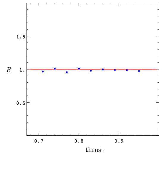
FIG. 2.: Ratio $R$ of the order $\alpha_{s}^{2}$ contribution to the thrust distribution as calculated here to the same quantity as calculated by Kunszt and Nason, Ref. [5]. The horizontal lines represent the expected result, 1, with an error estimate. The error bars on the computed points represent statistical errors. There is some correlation expected between neighboring points.

Outlook. Substantial effort will be required to test the computer code used for Fig. 2 in order to detect and remove any bugs that it may contain and then to document the code and the algorithms used. This work will be reported in future papers. With this code in hand, or with improved code from other authors, one can attack more difficult problems than discussed here. It remains to be seen for what problems the completely numerical method will prove to be more powerful than the analytical/numerical method that has served us so well up to now.

I thank U. Amaldi for initial encouragement to somehow do better with QCD calculations, L. Surguladze for advice on Feynman numerators, Z. Kunszt and P. Nason for help with the comparison to the results [5], and T. Sjostrand for advice about future applications. This work was supported by the U. S. Department of Energy.

REFERENCES

- [1] R. K. Ellis, W. J. Stirling, and B. R. Webber, QCD and Collider Physics (Cambridge, 1996); G. Sterman et al. (CTEQ Collaboration) Rev. Mod. Phys. 67, 157, (1995).
- [2] R. K. Ellis, D. A. Ross, and A. E. Terrano, Nucl. Phys. B178, 421 (1981).
- [3] Z. Kunszt and D. E. Soper, Phys. Rev. D 46, 192 (1992).
- [4] G. Sterman, Phys. Rev. D 17, 2773, 2789 (1978).
- [5] Z. Kunszt, P. Nason, G. Marchesini and B. R. Webber in Z Physics at LEP1, Vol. 1, edited by B. Altarelli, R. Kleiss ad C. Verzegnassi (CERN, Geneva, 1989), p. 373
- [6] The preliminary code, beowulf Version 0.7, is available at http://zebu.uoregon.edu/~soper/beowulf.