| MADPH-98-1056 |
| FERMILAB-PUB-98/128-T |
| April 1998 |
Excited glue and the vibrating flux tube
Theodore J. Allen and M. G. Olsson
Department of Physics, University of Wisconsin,
1150 University Avenue, Madison,
WI 53706
Siniša Veseli
Fermi National Accelerator Laboratory,
P.O. Box 500, Batavia,
IL 60510
Abstract
Recent lattice results for the energy of gluonic excitations as a function of quark separation are shown to correspond to transverse relativistic flux tube vibration modes. For large quark separations all states appear to degenerate into a few categories which are predicted uniquely, given the ground state.
Introduction
Mesons in which the gluons are in an excited state have been discussed for some time. There are two main pictures that have evolved for treating these excited states. The first is the constituent gluon approach where the quarks and a gluon move in an MIT bag [1] or a potential model [2, 3]. The second picture envisions the quarks to be connected by a string or flux tube [4, 5, 6] which has quantized transverse vibrations. In this case the flux tube can be thought of as a coherent gluonic state. In all of these models the resulting meson is analogous to the diatomic molecule where the gluonic degrees of freedom are the “electronic state” that can assume many levels of excitation. Each excited state yields an interaction energy that acts as an adiabatic potential in which the quarks or “ions” move. The ground state of the glue corresponds to standard meson states and the excited glue to “hybrid meson” states.
Recently the excited glue states with fixed end points have been investigated in detail by lattice simulation [7]. These calculations are done with an improved action in the quenched approximation for a variety of gluonic operators, and on several anisotropic lattices. It is our purpose here to point out that the systematics of the gluon states are extremely simple from the vibrating relativistic flux tube point of view. To a remarkable extent the gluon states group themselves into a few highly degenerate states at large quark separations, reflecting the well known degeneracy of the quantized two-dimensional harmonic oscillator.
We further show that, given the ground state potential, the hybrid adiabatic potentials are uniquely predicted and agree well with the lattice results. Our calculation is fully relativistic and does not introduce arbitrary procedures as required by previous work [4].
Relativistic strings
It is a common misconception that a free relativistic string must be formulated in twenty six dimensions in order to be consistently quantized. In fact, quantized theories of a single non-interacting relativistic string can be defined consistently in any spacetime dimension smaller than twenty six using the standard string theoretic methods. Long ago, Brower and Goddard and Thorn [8] showed that free bosonic string theories in spacetime dimensions are free of ghost (negative norm) states as long as the first excited state is not tachyonic. Subsequently Rohrlich [9] found an oscillator quantization of the non-interacting relativistic string that is manifestly free of ghosts in any dimension, while Polyakov [10] quantized the string as a sum over random surfaces that is consistent in dimensions twenty-six or smaller. It is only in the context of dual models and their superstring offspring that the theory becomes consistent in a single (critical) dimension. This is because unphysical states that may be consistently eliminated from a free string cannot be consistently eliminated from an interacting string theory [11].
The Nambu-Goto action, with fixed end boundary conditions may be quantized consistently in using the Gupta-Bleuler method in the temporal gauge, . The energy of a string of tension and distance between the fixed ends,
| (1) | |||||
| (2) |
follows from the zero mode of the Virasoro constraint [12, 13]. The index labels the mode level which is occupied by phonons of positive helicity and phonons of negative helicity. The constant is an arbitrary normal ordering constant subject only to the constraint, , of the no-ghost theorem.
In the temporal gauge, Lorentz invariance does not impose any restriction on spacetime dimension [9] as it does in light-cone gauge and only requires that be chosen such that the system has a rest frame. This formally infinite constant is often calculated [14, 15, 16] by summing the Casimir zero-point energies using zeta function regularization, yielding the value . The standard BRST quantization method also yields the values and . The Gupta-Bleuler method we use here yields a consistent quantum theory of a single string for any value of . It is well known that different methods of quantizing theories with constraints, such as the Nambu-Goto string, need not be equivalent and may differ in their energy spectra as well as in their dynamical degrees of freedom.
The excited glue states are completely specified by the separation between the ends and the occupation number of each of the modes, . These states can be labeled in molecular notation [17] by three quantities. The first is their angular momentum along the quark axis,
| (3) |
States with are denoted . The second label is the CP value of the glue which appears as either a subscript or depending on whether CP is even or odd respectively. The states () are labeled additionally by a superscript denoting their parity under reflection through a plane in which the axis lies. The CP value of the flux tube is determined by [4]
| (4) |
In the vibrating flux tube model the and states are always degenerate as well.
For and the glue states are uniquely and respectively. For the flux tube can be excited in the , , and states. For an arbitrary , states with can be excited. This degeneracy is a firm prediction of the flux tube picture and is expected to hold for large separations.
Testing the flux tube vibration picture
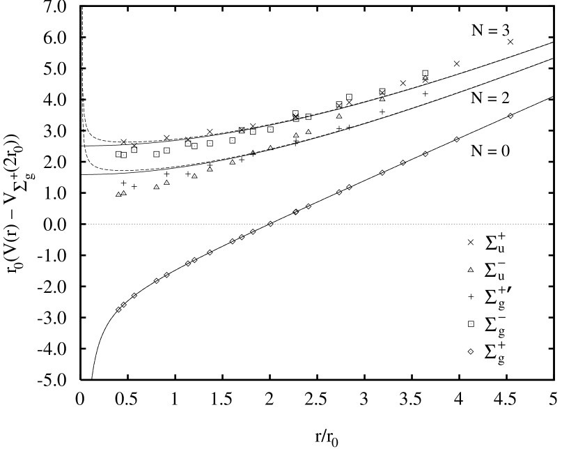
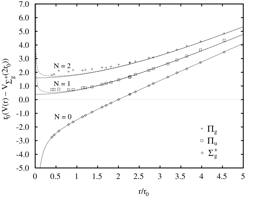
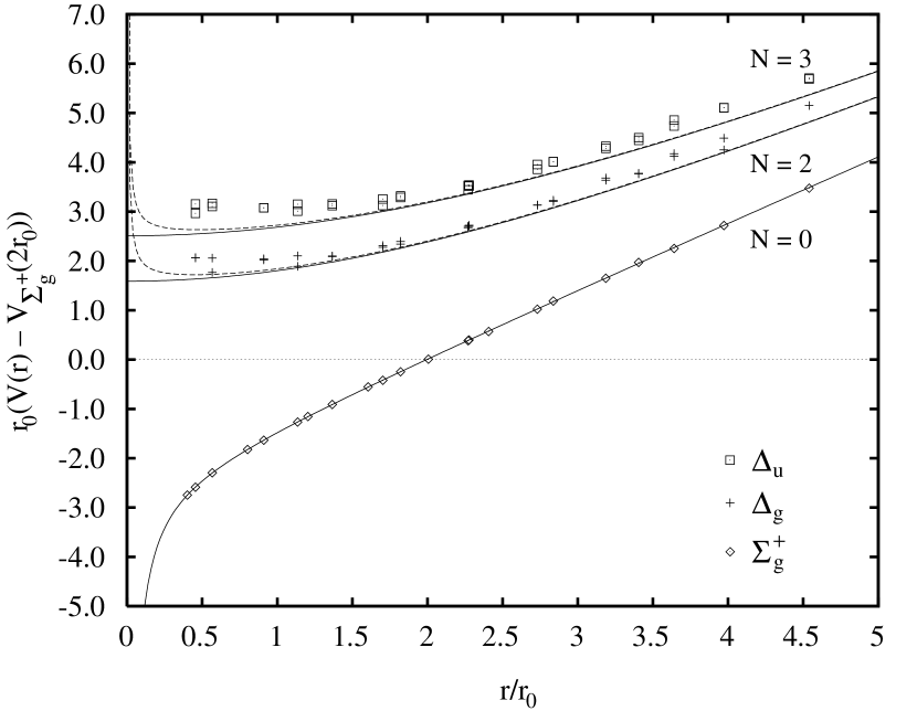
In this section we compare the predictions of Eq. (1) for flux tube vibrations with the results of a lattice simulation of quenched QCD [7]. The lattice energies are given relative to the ground state () energy at a quark separation of , where is a hadronic scale distance determined [18] from the data at large .
The ground state () potential from Eq. (1) with , together with a short distance color singlet potential and an additive constant, gives
| (5) |
The existence of a potential for all values of requires non-negative. If , the “Cornell” potential is recovered,
| (6) |
The best fit of Eq. (5) to the lattice data occurs in fact where . Assuming this, we obtain for the best representation of
| (7) | |||||
Once the above values have been fixed by the ground state lattice data, all of the excited states are predicted uniquely, with
| (8) |
The gluonic excitation energies obtained by lattice simulation are shown in Figs. 1–3 in molecular notation. In Fig. 1 the states are plotted. The lowest () and () states are displayed in Figs. 2 and 3 respectively. For , the and states are degenerate.
In the figures we also show the , , and predictions superimposed upon the , , and lattice data [7]. We observe general agreement at large . The and states follow the vibrating string prediction even down to small separations. The states do not closely resemble either the or curves. One possible explanation is that they have admixtures of higher excitations.
Because the flux tube may be viewed as a coherent gluonic state, one might expect that for small quark separation it should continue smoothly to the perturbative configuration of one gluon and a color octet. We test this assumption by modifying the prediction of Eq. (8) by adding to the excited potentials a color octet short distance repulsion,
| (9) |
where was determined (Testing the flux tube vibration picture) by the short distance color singlet attraction of the ground state. Our results (dashed curves) indicate that this short range behavior seems to improve most of the predictions, if only marginally.
Conclusions
Relativistic vibrating string models have been widely discussed in the literature. Some authors maintain that a tachyonic ground state () is required in fewer than 26 dimensions [15, 16, 19, 20]. Others maintain that there are quantization ambiguities that allow, at least for a non-interacting string, consistent quantization in four dimensions [8, 9, 12, 21]. We advocate the later interpretation and show that the vibrating (phonon) excitations closely correspond to a lattice simulation of QCD.
The success of this simple flux tube picture strongly supports the string vibration modes as being the correct low energy degrees of freedom for the gluonic excitations in hybrid mesons. The original work of Isgur and Paton [4] has the same large limit as our result but is intrinsically non-relativistic. Since waves propagate with the speed of light on a flux tube, a relativistic model is mandated. Furthermore, the Isgur-Paton model introduces an arbitrary radial functional dependence to avoid unphysical behavior at . In this function a free parameter can be tuned so that the potential has zero slope at for the state. For larger the intercept rises as required, but now the slope becomes progressively more negative. This effect is demonstrated numerically in [3]. Our model predicts a unique potential for the excited states once the parameters are determined by the ground state.
Acknowledgements
We thank C.J. Morningstar for providing us the data of reference [7]. This work was supported in part by the US Department of Energy under Contracts Nos. DE-AC02-76CH03000 and DE-FG02-95ER40896.
References
-
[1]
T. Barnes, Caltech Ph.D. thesis, 1977;
P. Hasenfratz, R.R. Horgan, J. Kuti, and J.M. Richard, Phys. Lett. 95B (1981) 299;
K.J. Juge, J. Kuti, and C.J. Morningstar, “Bag picture of the excited QCD vacuum with static source,” hep-lat/9709132. -
[2]
D. Horn and J. Mandula, Phys. Rev. D17
(1978) 898;
T. Barnes, Z. Phys. C10 (1981) 275;
J. Cornwall and A. Soni, Phys. Lett. 120B (1983) 431. - [3] E. S. Swanson and A. P. Szczepaniak, “Heavy hybrids with constituent gluons,” hep-ph/9804219.
- [4] N. Isgur and J. Paton, Phys. Rev. D31 (1985) 2910.
-
[5]
J. Merlin and J. Paton, J. Phys. G:
Nucl. Phys. 11 (1985) 439; Phys. Rev. D35
(1987) 1668; Phys. Rev. D36 (1987) 902;
I. Zakout, R. Sever, Z. Phys. C75 (1997) 727. - [6] S. Perantonis and C. Michael, Nucl. Phys. B347 (1990) 854.
- [7] K.J. Juge, J. Kuti, and C.J. Morningstar, Proceedings of the XVth International Symposium on Lattice Field Theory, Nucl. Phys. B (Proc. Suppl.) 63 (1998) 326; hep-lat/9709131.
-
[8]
R.C. Brower,
Phys. Rev. D6 (1972) 1655;
P. Goddard and C.B. Thorn, Phys. Lett. 40B (1972) 235. - [9] F. Rohrlich, Phys. Rev. Lett. 34 (1975) 842; Nucl. Phys. B112 (1976) 177.
- [10] A.M. Polyakov, Phys. Lett. 103B (1981) 207.
- [11] M.B. Green, J.H. Schwarz, and E. Witten, “Superstring theory,” (Cambridge University Press, Cambridge, 1987)
- [12] V.V. Nesterenko, Theor. Mat. Fiz. 71 (1987) 238.
- [13] T.J. Allen, M.G. Olsson, and S. Veseli, in preparation.
- [14] L. Brink and H.B. Nielsen, Phys. Lett. 45B (1973) 332.
- [15] G. Lambiase and V.V. Nesterenko, Phys. Rev. D54 (1996) 6387.
-
[16]
O. Alvarez, Phys. Rev. D24 (1981) 440;
J.F. Arvis, Phys. Lett. 127B (1983) 106. - [17] L.D. Landau and E.M. Lifshitz, “Quantum Mechanics,” (Pergamon Press, Oxford, 1977)
- [18] C. Morningstar and M. Peardon, Phys. Rev. D56 (1997) 4043.
- [19] J. Polchinski and A. Strominger, Phys. Rev. Lett. 67 (1991) 1681.
- [20] K.R. Dienes and J.-R. Cudell, Phys. Rev. Lett. 72 (1994) 187.
- [21] A. Patrascioiu, Nucl. Phys. B81 (1974) 525.