Non-Equilibrium Field Theory Dynamics in Inflationary Cosmology

Abstract

For simple inflationary models, we provide a consistent and complete scheme by which the macro-physical details of early universe inflation may be determined explicitly from the underlying micro-physical theory. We examine inflationary dynamics within the context of a fully renormalized, non-perturbative, and non-equilibrium quantum field theory using the closed time path formalism. We study the non-perturbative dynamics using the self-consistent Hartree approximation and the large $N$ limit. In addition, we include gravitation dynamically by means of the semi-classical approximation to Einstein gravity, allowing the cosmological geometry to be determined self-consistently by the evolution of the particle fields. We develop a simple and numerically implementable regularization and renormalization scheme for which the renormalization counterterms contain no explicit dependence on the initial state.

We concern ourselves first with the dynamics of new inflation models, showing how the dynamics become quantum fluctuation driven. We then describe how these quantum fluctuations may be reassembled into an effective field which behaves classically and acts as the source for the gravitational background. This allows us to determine the spectrum of primordial density perturbations in a consistent manner. We also examine explosive particle production after inflation through the processes of spinodal decomposition and parametric amplification, showing that the non-perturbative backreaction on the inflaton field prevents catastrophic particle production. We find a strong dependence of particle production on the expansion rate and on the symmetry properties of the inflaton.

Preface

Cosmology, the study of the beginnings of the Universe, has been a subject of study and speculation for thousands of years. We now live in a remarkable era in which cosmology has become an analytical subject of research to be studied, observed, and understood by science.

Observations of the universe today have led to a description of the universe back to times of less than a tiny fraction of a second after the beginning of time. The most important advance in the study of our universe has been the construction of the Standard Cosmological Model. In analogy to the Standard Model of Particle Physics, this Model provides the framework around which all known aspects of Cosmology fit.

The Standard Cosmology states that we live in an expanding universe in which, on the largest of scales, each point is like any other. While the details of the cosmology, such as the exact size, shape, and total content of matter, are yet to be determined, the uniformity of our universe has been verified to remarkable accuracy by relatively recent observations.

The remarkable success of this model leads one to ask a very simple question: Why is the universe so uniform? It is an incredible fact that science has arrived at an answer on the basis of what is known about high energy physics and gravitation. The answer: Inflation.

The solution to such a profound question deserves scrutiny and attention. The purpose of this dissertation is to examine what is known about inflation, to question its assumptions, and to carefully analyze its consequences and predictions.

Acknowledgments

This work was made possible by the hard work, dedication, and support of a large network of individuals. At the focal point of this network are a number of people I would like to acknowledge for their extraordinary efforts on my behalf. First and foremost I thank my advisor, Rich Holman, not only for leading me on the road to becoming a scientist, but also for pointing out all the overgrown paths and encouraging their exploration, even when it may not be the safest route. Rich has a true love of knowledge, which becomes contagious when combined with his outstanding ability to communicate ideas at all levels.

I have been very lucky to have not just one advisor, but two, as Dan Boyanovsky has often taken on that role. Dan is full of knowledge, but what has most impressed me is his eagerness to share his ideas and to listen to the ideas of others. He has uncommon patience, and the ability to transform a vague concept into a detailed project.

I have also benefited a great deal from collaboration with Hector de Vega. My extensive email communications with Hector led to a much greater understanding of many of the details in this thesis. I have enjoyed the opportunities I have had to work with him, and I hope to continue our collaborations into the future.

I would also like to thank Ling-Fong Li and Martin Savage for the important roles they played in my education. I thank Bob Griffiths for his curiosity and for making me explain even those aspects of cosmology of which I am unsure, and Bob Nichol for providing the perspective that only an observational cosmologist can provide. I would be amiss if I did not thank the great staff of the physics department, in particular Nancy Watson, Mary Shope, Lori Marcus, Chuck Gitzen, Cheryl Wehrer, Pricilla Jarrett, Terri Jones, and Mary Placeway. A special bit of thanks goes to Joe Rudman, who was invaluable in helping me recover my thesis after I deleted it from the hard drive. For their discussions, I thank Prem Kumar and Anupam Singh, as well as most of the other graduate students in the department who have provided a stimulating atmosphere in which to work.

Particular thanks go to good friends, who have provided so much support – Mark Mattson, Phil Koran, Eldon Decker, and especially James Walden and Elaine Kirkpatrick. My greatest thanks go to my wife Johanna who makes each and every day the best day of my life.

G’dalm K’ding

Contents

1. 1 Introduction
   1. 1.1 The Need for a Non-equilibrium Description
   2. 1.2 Previous Research in Non-equilibrium Quantum Field Theory
   3. 1.3 Content of the Thesis
2. 2 Field Theory in FRW Spacetime
   1. 2.1 Introduction to FRW Spacetime
   2. 2.2 Shortcomings of the Standard Cosmology
   3. 2.3 Introduction to Inflation
   4. 2.4 Field Theory in FRW Spacetime
   5. 2.5 Metric Perturbations
3. 3 Non-equilibrium Field Theory
   1. 3.1 Introduction to the Closed Time Path Formalism
   2. 3.2 Field Equations in FRW
      1. 3.2.1 Real Scalar Field: Hartree Dynamics
      2. 3.2.2 $O(N)$ Scalar Field: Large $N$ Dynamics
      3. 3.2.3 Density Matrix Formalism
      4. 3.2.4 Gravitational Dynamics
   3. 3.3 The $\lambda\Phi^{4}$ Theory
   4. 3.4 Renormalization and Energy Momentum
4. 4 New Inflation
   1. 4.1 Introduction and Motivation
   2. 4.2 Analysis
      1. 4.2.1 Early time dynamics
      2. 4.2.2 Classical or quantum behavior?
      3. 4.2.3 Numerics
   3. 4.3 Zero Mode Assembly
   4. 4.4 Scalar Metric Perturbations
   5. 4.5 Decoherence: Quantum to Classical Transition During Inflation
   6. 4.6 Conclusions
5. 5 Explosive Particle Production After Inflation
   1. 5.1 Introduction
   2. 5.2 Evolution
      1. 5.2.1 Early Time Solutions for Slow Roll
      2. 5.2.2 Numerical Analysis
      3. 5.2.3 Late Time Behavior
   3. 5.3 Conclusions
6. 6 Conclusions

Chapter 1 Introduction

The ultimate goal of studies of the early universe is the ability to accurately predict the macro-physical properties of the universe from a micro-physical description. This is a daunting task which requires the relation of the full dynamics of the underlying quantum field theory to the geometrical dynamics of gravity. This evolution must then be followed over an extraordinary dynamic range before the results may be interpreted to yield concrete predictions for observable properties of today’s universe.

Such a program requires a number of features:

• The ability to evolve quantum fields dynamically without any assumptions of an equilibrium state.

• The ability to treat states of extremely high (non-perturbative) energy densities.

• The ability to evolve gravity in a manner self-consistent with the evolution of the quantum fields.

• The ability to interpret the results of the quantum field theory dynamics.

In addition to these fundamental features, one must be concerned with the renormalization aspects of the field theory and also have means to explicitly evaluate the dynamics through analytical and numerical means.

For a class of simple models, we have developed such a program. In the following pages, we apply this program to inflationary cosmology.

1.1 The Need for a Non-equilibrium Description

Non-equilibrium field theory[1], which describes the dynamical evolution of quantum fields, has become an important tool in particle physics and cosmology. The ability to compute observables in highly dynamical situations in which the results of ordinary equilibrium field theory fail, is necessary in order to gain a better understanding of a wide number of phenomena, including phase transitions in condensed matter systems and at particle accelerators[2]. Perhaps the most important applications of non-equilibrium field theory, however, are to phenomena of the early universe[3, 4, 5, 6, 7].

The reason it is necessary to go beyond traditional equilibrium techniques in describing cosmology is the extreme environment of our universe at early times[8, 9]. It is now well accepted that early in its history, our universe was very hot with energy densities approaching the Planck scale, while the universe was rapidly cooling due to expansion. As a result of the rapid cooling, it is expected that matter goes through a number of phase transitions before we reach the present state of our universe[10, 11, 12, 13].

Unless the matter fields involved in these phase transitions interact at a rate much greater than the cooling rate of the universe, the evolution proceeds out of equilibrium. This non-equilibrium evolution may in turn have a number of important physical consequences. One example is baryogenesis[14]. If one assumes that the universe began in a state with equal numbers of baryons and anti-baryons, then it is necessary to have some process in the history of our universe which results in a biased production of baryons over anti-baryons. Such a process, which may have occurred during the electroweak phase transition or at an earlier time, requires a departure from equilibrium since baryons and anti-baryons are produced in equal numbers in any equilibrium process.

Another example of a non-equilibrium process in the early universe is the production of topological defects during a phase transition[15]. Just as the domain structure in a ferromagnet is very different when the sample is cooled adiabatically through the Curie temperature compared to a sample which is rapidly cooled, the production of topological defects depends strongly on the cooling rate of the universe[16]. Again, equilibrium analyses will not provide an accurate picture of defect formation.

The phenomena to be studied here, inflation[17, 18, 19, 20, 21] and the subsequent phase of parametric amplification[22, 23, 24], are likewise phenomena of a non-equilibrium nature[25, 26, 27, 28, 29, 30]. Inflation, and the near exponential expansion which characterizes it, can only occur if the state of the inflating universe differs from its equilibrium state. Furthermore, it is the dynamical evolution which allows inflation to end. Parametric amplification similarly relies on the rapid evolution of a quantum field to produce a parametric resonance of field quanta. A field in equilibrium shows no such behavior.

Despite the non-equilibrium nature of these phenomena, the bulk of the work treating the processes has utilized equilibrium techniques, most notably the effective potential[31]. The effective potential is the name given to the equilibrium free energy of a system and while it is a very useful quantity in determining a number of important properties, such as the equilibrium ground state of the system, it is ineffective in describing the dynamics of the system[32]. It therefore becomes necessary to move beyond equilibrium techniques and to analyze the dynamics of these phenomena using non-equilibrium field theory.

1.2 Previous Research in Non-equilibrium Quantum Field Theory

With the recognition of the importance of non-equilibrium techniques, a significant literature has developed which deals with techniques, approximations, and applications of non-equilibrium field theory as applied to the early universe.

The work of Hu and Calzetta and their collaborators[3] has focused primarily on the formal issues of non-equilibrium field theory, with an emphasis on statistical field theories. The Langevin approach derived from the influence functional has been shown to be a useful tool in studying the early universe[3]. It should be noted, however, that statistical field theory remains an approximation to the full quantum field theory. Other important contributions of this research group include the study of the non-perturbative $1/N$ expansion for models with overall $O(N)$ symmetry. In the context of the closed time path treatment of full quantum field theory, this work has included an analysis which places the large $N$ and other approximations within the context of the computation of the full two-particle irreducible (2PI) Green’s functions[33, 34, 35]. Much of their work has been completed in expanding spacetimes and has included the issues of renormalization as well as important applications. Of particular interest here is the work of Ramsey and Hu which treats the $O(N)$ theory in Friedmann-Robertson-Walker (FRW) spacetime including renormalization[34], and applies the formalism to post-inflationary parametric resonance[35], reproducing and verifying many of the results of Refs. [36, 29], which are included here in Ch. 5.

Another research group with important contributions to the subject is the Field Theory group at the Los Alamos National Laboratory[37, 38, 39, 40]. Their contributions include work on the $1/N$ expansion, including a determination of the next-to-leading order contributions in Minkowski spacetime as well as work on the leading order approximation in FRW spacetime[38]. Other important contributions are provided by their non-equilibrium study of symmetry breaking[39]. Also of importance to the present work is their analysis of the non-perturbative Hartree and large $N$ approximations as compared to exact results in a toy quantum mechanics problem, which provides some indication as to the reliability of the approximations we use in our analysis[40].

The research which forms the foundation of the present work, however is that of Boyanovsky, de Vega, and Holman and their collaborators[25, 26, 28, 41]. This important work includes the non-equilibrium study of symmetry breaking[41] and domain formation in scalar field theories[28] and also includes important contributions to the formalism of non-equilibrium quantum field theory and its renormalization in FRW spacetime[26]. In addition, the ground breaking work in collaboration with Lee and Singh on reheating[42] is an important piece of the puzzle, which along with the present work, paints a complete picture of inflation from its earliest stages to its end, and on to the subsequent phases of the universe.

Of course, all of the recent work in this area is grounded in the early pioneering work on non-equilibrium field theory[1] and the study of quantum fields in curved spacetime[43] which will be reviewed in further detail in Ch. 2.

1.3 Content of the Thesis

In this work we develop the techniques of non-equilibrium quantum field theory in conformally flat FRW spacetime, including non-perturbative approximation techniques and the introduction of a novel renormalization scheme which provides a simple interpretation of the renormalizations and allows for numerical analysis of the dynamics of quantum fields in both fixed and dynamically evolving FRW spacetimes[26, 36, 29, 27, 30]. We then provide two new applications of these techniques to important phenomena of the early universe: new inflation[27, 30] and post-inflationary parametric amplification[36, 29].

We begin our study in Ch. 2 with a review of FRW spacetime[8, 9, 44] and the basics of field theory in an expanding universe[43]. We describe the observational support for an FRW description including evidence for the important properties of homogeneity and isotropy and also provide the basics of the geometry of such a universe as described by general relativity. Next, we examine potential shortcomings of this standard picture, in the horizon, flatness, and relic problems, before moving on to the concept of inflation. Here, we describe how inflation provides solutions to the problems of FRW cosmology and discuss the elements necessary to a successful implementation of inflation. As we shall see, this will lead to the introduction of quantum field theory which in turn provides the particularly interesting prospect that the same elements yielding inflation may also result in the very metric perturbations from which the large scale structure of our universe formed. We then introduce the basic concepts of field theory in FRW spacetime, including the introduction of conformal coordinates and a short discussion of renormalization in FRW spacetime. Finally, we complete the chapter with a short discussion of the formalism and physics of metric perturbations[45, 46].

We follow our discussion of field theory in FRW spacetime with an in depth study of the techniques of non-equilibrium field theory in Ch. 3. First, we introduce the basic formalism before detailing the models and approximations we will find useful in our studies of the early universe. We pay particular attention to the non-perturbative Hartree[47, 26] and large $N$[48, 49, 50, 38, 27, 34] approximations, deriving the appropriate equations of motion and describing in detail the important properties and limitations of these tools. Next, we examine the initial conditions which will be used to begin the evolution of the dynamics when we apply our formalism to practical problems. This oft neglected detail will be seen to be of particular significance to both formal and practical issues of non-equilibrium field theory in FRW spacetime[51]. The renormalization of the field theory is another issue of importance, especially when it will become necessary to numerically solve the equations of motion in a particular model. We show in detail how we arrive at our renormalization scheme and discuss the usefulness of our approach, while pointing out the important connection between the initial conditions for the field theory and its renormalization. Finally, we provide a description of the semi-classical approximation to gravity[43], which allows one to determine the dynamics of the scale factor describing the classical expansion of the universe self-consistently in terms of the evolution of the quantum fields of that universe. Such a description will also require us to make a number of additional renormalizations.

Having dispensed with the details of the formalism of non-equilibrium field theory in FRW spacetime, Chs. 4 and 5 deal with applications of the techniques developed in Chs. 2 and 3. First, we examine the process of new inflation[52, 53, 27, 30], beginning with a discussion of what the basic scenario is, why it was introduced, and what the problems with the scenario are. This leads into the introduction of the particular model of new inflation we study as well as a discussion of initial conditions. Next, we provide the analytical results of the dynamics of new inflation, followed by the details and results of our numerical study[27, 30]. The chapter is completed by a discussion of the dynamical assembly of a classical object which may be interpreted as driving the inflationary phase, followed by the details of the formation of metric perturbations and the de-coherence properties of the quantum field theory[30].

Our second application, discussed in Ch. 5, is the analysis of the phase of explosive particle production which may have occurred after a phase of inflation [23, 24, 25, 54, 55, 56, 36, 29, 57, 58, 59, 60, 61]. We begin with a description of the basic scenario of chaotic inflation. We then analyze within our models the dynamics of phases of particle production due to the phenomena of spinodal decomposition and parametric amplification, including both analytical and numerical results[36, 29]. We conclude with a discussion of the significance of our results in the context of reheating.

Finally, we present our primary conclusions in Ch. 6, discussing the importance of this work to our understanding of cosmology and its interactions with particle physics. We also discuss a number of other applications such as baryogenesis and defect formation which may benefit from a fully non-equilibrium analysis.

Chapter 2 Field Theory in FRW Spacetime

2.1 Introduction to FRW Spacetime

The so-called standard cosmology presents a remarkably successful picture of our universe[9, 62]. It is based upon two primary assumptions:

1. The universe is homogeneous and isotropic on large scales.

2. The geometry of the universe is determined by general relativity.

Taken together, these properties yield a Friedmann-Robertson-Walker (FRW) cosmology [63, 64, 65].

The conditions of homogeneity and isotropy are very restrictive. If we define $h_{ij}$ to be the metric on the three-dimensional surface defined by the spatial sections on the full four-dimensional spacetime, such that the differential spatial distances are given by

$$d{\vec{l}}^{2}=h_{ij}dx^{i}dx^{j}\;,$$ (2.1)

then we can define the spatial Riemann curvature tensor $R^{(3)\;l}_{ijk}$. Given the connection corresponding to the metric $h_{ij}$

$$\Gamma^{k}_{ij}\equiv\frac{1}{2}h^{kl}\left[\partial_{i}h_{jl}+\partial_{j}h_{il}-\partial_{l}h_{ij}\right]\;,$$

the Riemann tensor is

$$R^{(3)\;l}_{ijk}=\partial_{j}\Gamma^{l}_{ik}-\partial_{i}\Gamma^{l}_{jk}+\Gamma^{m}_{ik}\Gamma^{l}_{mj}-\Gamma^{m}_{jk}\Gamma^{l}_{mi}\;.$$ (2.2)

The property of isotropy, which in fact, includes the property of homogeneity if required at every spatial point, requires that the spatial curvature defined in this way is constant. That is,

$$R^{(3)\,kl}_{ij}={\cal K}\left[\delta^{k}_{i}\delta^{l}_{j}-\delta^{k}_{j}\delta^{l}_{i}\right]\;,$$ (2.3)

where the inverse metric $h^{ij}$ has been used to raise indices.

The constant ${\cal K}$ may take on any value, but there are just three different cases corresponding to different topologies for the universe. If ${\cal K}$ is negative, then the spatial sections take on a hyperbolic form. These may be defined as the three-dimensional surfaces embedded in a four dimensional Minkowski spacetime given by the relation

$$t^{2}-x^{2}-y^{2}-z^{2}=R^{2}\;,$$

where $R$ is an arbitrary constant. The second case is ${\cal K}=0$, which means that at every point in the space, the curvature is zero. The spatial sections are flat and are therefore given by the three dimensional Euclidean metric. Finally, ${\cal K}$ may be positive, corresponding to spatial sections of spherical form. We may define these by embedding them in a four dimensional Euclidean space. They are given by the relation

$$w^{2}+x^{2}+y^{2}+z^{2}=R^{2}\;.$$

Again, $R$ is an arbitrary constant.

These three cases may be conveniently combined in the full four dimensional spacetime metric

$$ds^{2}=g_{\mu\nu}dx^{\mu}dx^{\nu}=dt^{2}-a^{2}(t)d\vec{l}^{2}\;,$$ (2.4)

where $d\vec{l}$ is the differential element giving the spatial sections and the scale factor $a(t)$ is, for now, an arbitrary function of time. The spatial metric may be written in spherical coordinates as

$$d\vec{l}^{2}=\frac{dr^{2}}{1-Kr^{2}}+r^{2}d\theta^{2}+r^{2}\sin^{2}(\theta)d\phi^{2}\;.$$ (2.5)

Here, $K\equiv{\cal K}/|{\cal K}|$ takes on the discrete values $K=-1,0,+1$ corresponding to the cases of hyperbolic, flat, and spherical spatial sections respectively. We see that in the flat case of $K=0$, the spatial metric may be written in Cartesian coordinates as

$$d\vec{l}^{2}_{(K=0)}=dx^{2}+dy^{2}+dz^{2}\;.$$

The metric of the form given by (2.4) and (2.5) describing a homogeneous and isotropic cosmology is referred to as a Robertson-Walker metric[64, 65]. For a formal derivation of this important piece of the standard model, we refer the reader to the book by Wald[44]. Further discussions are given in the books by Weinberg[62] and Peebles[9]. The latter reference also provides a nice discussion of the many equivalent coordinatizations of the Robertson-Walker metric including conformal coordinates, which are of particular importance and will be discussed in Sec. 2.4.

The second of the primary assumptions of the standard cosmology determines the dynamics of the scale factor $a(t)$ in terms of the matter content of the universe. General relativity[62, 44] is based upon Einstein’s equation relating the spacetime curvature to the energy-momentum $T_{\mu\nu}$. The full Riemann curvature tensor, $R_{\alpha\beta\gamma}^{\delta}$, for the four dimensional spacetime is defined in terms of the spacetime metric $g_{\mu\nu}$ in complete analogy to the spatial curvature (2.2). The connection on the spacetime manifold is defined as

$$\Gamma^{\rho}_{\mu\nu}\equiv\frac{1}{2}g^{\rho\sigma}\left[\partial_{\mu}g_{\nu\sigma}+\partial_{\nu}g_{\mu\sigma}-\partial_{\sigma}g_{\mu\nu}\right]\;,$$

and the curvature tensor is

$$R_{\mu\nu\rho}^{\sigma}=\partial_{\nu}\Gamma^{\sigma}_{\mu\rho}-\partial_{\mu}\Gamma^{\sigma}_{\nu\rho}+\Gamma^{\alpha}_{\mu\rho}\Gamma^{\sigma}_{\alpha\nu}-\Gamma^{\alpha}_{\nu\rho}\Gamma^{\sigma}_{\alpha\mu}\;.$$

Appearing in Einstein’s equation is the Einstein curvature tensor $G_{\mu\nu}$, constructed from the Ricci tensor

$$R_{\alpha\beta}\equiv R_{\alpha\mu\beta}^{\mu}$$

and the Ricci scalar

$${\cal R}\equiv R^{\alpha}_{\alpha}\;.$$

With these definitions, Einstein’s equation reads

$$G_{\mu\nu}\equiv R_{\mu\nu}-\frac{1}{2}g_{\mu\nu}{\cal R}=-8\pi G_{N}T_{\mu\nu}\;,$$ (2.6)

where the proportionality constant $G_{N}$ is Newton’s gravitational constant, which in natural units is related to the Planck mass by the equation $G_{N}=1/m_{Pl}^{2}$.

Given the metric (2.4) with (2.5), Einstein’s equation reduces to just two independent equations of motion for the scale factor:

$$G^{0}_{0} = -3\frac{\dot{a}^{2}}{a^{2}}-3\frac{K}{a^{2}}=-8\pi G_{N}T^{0}_{0}\;,$$ (2.7)

$$G^{1}_{1} = -2\frac{\ddot{a}}{a}-\frac{\dot{a}^{2}}{a^{2}}-\frac{K}{a^{2}}=-8\pi G_{N}T^{1}_{1}\;.$$ (2.8)

Note that the non-diagonal elements of both $G_{\mu\nu}$ and $T_{\mu\nu}$ are identically zero while the remaining diagonal elements simply reproduce Eq. (2.8). We therefore see that $T_{\mu\nu}$ must have the form of an ideal fluid with energy density $\rho\equiv T^{0}_{0}$ and pressure $p\equiv-T^{1}_{1}$ in order to be consistent with the homogeneity and isotropy conditions.

We can make a number of conclusions from the equations of motion (2.7) and (2.8). First, if we assume that $\rho>0$, we see that $\dot{a}^{2}/a^{2}>0$ and the universe is necessarily expanding (or contracting). Second, if $p\geq 0$ then $\ddot{a}/a<0$ and the universe decelerates with time

We should note that for ordinary matter and radiation, the energy and pressure densities, which satisfy the respective equations of state $p=0$ and $p=\rho/3$, are functions of the scale factor and therefore also of time. In particular, ordinary matter has an energy density inversely proportional to the physical volume and therefore changes with the scale factor as

$$\rho_{m}(t)\propto\frac{1}{a^{3}(t)}\;.$$

Similarly the energy density of radiation changes as

$$\rho_{r}(t)\propto\frac{1}{a^{4}(t)}\;,$$

which may be interpreted as a change in photon (or other massless particle) density proportional to $1/a^{3}(t)$ with an additional factor of $1/a(t)$ due to the redshifting of the photon frequency.

Given the properties of a dynamic, decelerating universe, if the universe is presently expanding, as we will provide support for below, then physical length scales were much smaller at earlier times, with the expansion rate increasing as one goes back. If one extrapolates such a scenario of expansion far enough back, then one arises at the conclusion that there is an instant of time at which all physical length scales are reduced to zero. This is the source of the concept of the big bang, which should not be interpreted as an explosion of matter into space as its name implies, rather it represents the rapid expansion of space itself from an initial state approaching zero size and infinite energy density.

Another property is that if the geometry of the universe is flat or hyperbolic with $K=0$ or $K=-1$ respectively, then an expanding universe expands forever. However, in the spherical case with $K=+1$, then at some instant in time $8\pi G_{N}\rho/3=K/a^{2}$ and the expansion halts after which the universe begins to contract. In this case, the universe eventually will return to a state approaching zero size and infinite energy density called the big crunch.

A final property of the expanding universe described by the standard cosmology that will be of particular interest is the existence of particle horizons. These exist because particles can travel at most at the speed of light. In particular, the furthest physical distance a light signal may have traveled at any time is given by

$$d_{H}(t)=a(t)\int^{t}\frac{dt^{{}^{\prime}}}{a(t^{{}^{\prime}})}\;.$$ (2.9)

This quantity is called the horizon distance. As we shall see, the important point is that if the scale factor grows no faster than linearly in $t$ as is the case in matter or radiation dominated cosmologies, then the horizon distance decreases faster than the scale factor as one goes to earlier times. This means that points which are in causal contact today may have been causally disconnected at earlier times. We will return to this important point in the next section.

Observational Support for the Standard Cosmology

The picture presented here of the standard cosmology has received substantial observational support, which has elevated the simple model to the level of a standard model. The support comes in three different areas:

1. Support for the theory of general relativity, especially on large scales.

2. Support for the expansion of the universe.

3. Support for the large scale homogeneity and isotropy of the universe.

We now review the most significant evidence supporting a standard cosmology description of our universe. Complete discussions may be found in Refs. [62, 9, 44].

Somewhat surprisingly, the element of support for the standard model which is perhaps the least certain is the theory of general relativity, largely because of the difficulties of verifying the theory on large scales. Of course, the success of general relativity on small scales is well known, beginning with the prediction and verification of the precession of the planet Mercury[66, 67]. To some extent, however, we must simply assume that general relativity is the correct theory of gravity on all cosmological scales.

Observational evidence for the expansion of the universe, on the other hand, is very extensive. The expansion was first observed by Hubble[68], who found that light emanating from distant cosmological objects was Doppler shifted toward the red part of the visible spectrum. Such redshifting indicates movement of objects away from our galaxy. Furthermore, Hubble observed that the amount of redshifting increases with the distance of the object. In particular, Hubble determined that there was a near linear relation between an objects redshift $1+z$, defined as the ratio of the observed wavelength to the expected wavelength for that source, and the distance $d$. This relationship is expressed as Hubble’s Law:

$$z\simeq H_{0}d\;,$$

where $H_{0}$ is Hubble’s constant.

While deficiencies in the ability of Hubble to accurately measure the distances of cosmological objects led to a value of $H_{0}$ an order of magnitude larger than recent determinations, Hubble’s Law itself is now well verified. We therefore know quite definitively that the universe is undergoing expansion.

The final piece of evidence in support of the standard cosmological model is direct observation of the homogeneity and isotropy of the large scale universe. The primary and most convincing observation in this regard is provided by the Cosmic Background Radiation (CBR) which was found to have an almost perfect blackbody spectrum at a temperature $T=2.73K$ with little variation in this temperature with the direction of the observation. In fact, if one subtracts the dipole component of the temperature variation, which may be explained by the movement of our reference frame with respect to the rest frame of the CBR, the temperature variation over the sky is of order $\delta T/T\sim 10^{-4}$. This means that at the time the photons making up the CBR last interacted with ordinary matter, the universe was homogeneous and isotropic to one part in 10,000. To better understand what this means, it helps to understand the source of the CBR.

Our standard picture of the early universe indicates that its temperature was once many orders of magnitude hotter than it is today. At high enough temperatures, we know that electrons dissociate themselves from protons. At such high temperatures, the radiation in the universe continually interacts with the charged electrons and protons, and photons are in a state of thermal equilibrium. However, as the universe cools, the electrons combine with the protons during a time called recombination (despite the fact that these particles were never combined before this time). Without the charged particles on which to scatter, the photons become effectively non-interacting. As a result, they simply free stream until they reach observers today.

In the meantime, the photons have redshifted with the expansion of the universe, and since a redshifted thermal (blackbody) spectrum remains thermal, we observe this cosmic background radiation as a near perfect blackbody spectrum at a temperature $T_{\gamma}$ given in terms of the photon temperature at recombination $T_{RC}$ by the relation

$$T_{\gamma}=\frac{T_{RC}}{(1+z)}\;.$$

The redshift at recombination is approximately $z\sim 1200$.

Since the ratio $\delta T/T$ is a constant for the cosmic radiation background during its evolution from recombination to today, it is clear that the recent observations of an isotropic and homogeneous CBR indicate that the universe was very isotropic and homogeneous at the time of recombination.

There are a number of other observations lending support to the model of an isotropic and homogeneous universe. The X-ray background, due to unresolved high redshift sources has been determined to be isotropic to about 5%. Similarly, the distribution of faint radio sources shows no preferential direction. Furthermore, the peculiar velocity field of galaxies on scales 50–100$Mpc$, which gives a direct measure of density variation through the movement of galaxies relative to the Hubble flow, provides a density contrast $\delta\rho/\rho\sim 0.1$.

Finally, galaxy distribution itself is found to be generally isotropic, although it is somewhat disconcerting that we have observed structure at even the largest observable scales. If the universe is truly isotropic on the largest scales then at some point we should reach a limit beyond which there are no new, larger structures.

2.2 Shortcomings of the Standard Cosmology

As we have seen, the standard cosmology is very well founded. However, it is not without problems. Obviously, the universe is not perfectly homogeneous since there are a number of individual structures ranging from planets to superclusters. These presumably form over time through gravitational instability, acting on the initially small density variations we observe in the CBR. However, the standard cosmology does not account for these density fluctuations, and it is fair to ask about their origin.

One of the most interesting challenges to the standard cosmology, on the other hand, is the question of how the universe could be so homogeneous in the first place. This would seem like an empty question given our assumptions of homogeneity were it not for the concept of particle horizons. As we saw in the preceding section, the horizon size in a matter or radiation dominated cosmology decreases relative to physical length scales as one goes to earlier times. This means that the horizon size at the time of recombination was much smaller than it is today, and there would have been no way in which correlations in the CBR in different directions could have formed.

In fact, each causal region at the time of recombination subtends less than a single degree of the presently observable universe and one might expect each of these causal regions to have evolved somewhat independently, resulting in a microwave background temperature spectrum which varies significantly from one region to the next. The actually observed homogeneity may, of course, be explained by simply assuming that the universe began in an almost exactly homogeneous state independent of particle interactions. However, we will see that there is a much more eloquent solution to the horizon problem based on a marriage of particle physics and cosmology.

A third problem of the standard cosmology is the relative flatness of our current universe. From the Friedmann equation (2.7), we see that there are two terms contributing to the expansion rate of the universe. The first is due to the energy density of matter and fields and the second is due to the curvature of the universe. It is convenient to introduce the critical density:

$$\rho_{c}(t)\equiv\frac{3}{8\pi G_{N}}\frac{\dot{a}^{2}(t)}{a^{2}(t)}\;.$$

If $\rho=\rho_{c}$, then we necessarily have a critical, spatially flat geometry while $\rho<\rho_{c}$ and $\rho>\rho_{c}$ correspond respectively to the open, hyperbolic geometry ($K=-1$) and the closed, spherical geometry ($K=+1$). This behavior is often summarized by the introduction of the single parameter $\Omega(t)\equiv\rho(t)/\rho_{c}(t)$, with $\Omega=1$ corresponding to the critical universe.

While the present value $\Omega_{0}$ is not well determined, through indirect measurement as a result of the successes of Big Bang Nucleosynthesis combined with a number of more direct measurement methods, it is restricted to the modest range $0.01\leq\Omega_{0}\leq 2.0$, while most cosmologists would agree that $\Omega_{0}$ is very likely to lie in the range $0.2\leq\Omega_{0}\leq 1$.

If, in addition to $\Omega$, we define the quantity $\Omega_{R}(t)\equiv-K/\dot{a}^{2}(t)$, Friedmann’s equation (2.7) becomes

$$\Omega(t)+\Omega_{R}(t)=1\;.$$ (2.10)

This equation displays a remarkable coincidence: given the accepted range of $\Omega$ and assuming $k\neq 0$ (that is, $\Omega\neq 1$), we see that the contributions of $\Omega$ and $\Omega_{R}$ to unity in Eq. (2.10) are within an order of magnitude or so of each other. What makes this so remarkable is that these two terms have a very different time dependence since $\Omega_{R}\propto 1/\dot{a}^{2}$ while $\Omega\propto 1/[\dot{a}^{2}(t)a(t)]$ for a matter dominated cosmology and $\Omega\propto 1/[\dot{a}^{2}(t)a^{2}(t)]$ for a radiation dominated cosmology. For these two quantities, which have drastically different time dependence, to be of the same order at this instant of time despite the huge variation of $a(t)$ of many, many orders of magnitude during the history of our universe is extraordinary. This coincidence is referred to as the flatness problem since it does not exist if the geometry of the universe is flat since that would mean $\Omega_{R}=0$.

Another way of posing this problem is to note that since $\Omega(t)$ decreases faster with expansion of the universe than $\Omega_{R}(t)$, the condition that these quantities now be within a couple of orders of magnitude of unity extrapolate back to the condition moments after the Big Bang of $\Omega(t_{Pl}\simeq 10^{-43}s)\sim 1\pm 10^{-60}$. This indicates an extreme fine tuning of the initial state of the universe.

The final problem of the standard cosmology arises as a result of the Grand Unified Theories (GUT’s) of particle physics. These theories, which unify all the known, non-gravitational forces of the universe, typically predict the production of topological defects. In particular, all known GUT’s predict the production of large numbers of monopoles which would quickly come to dominate the energy density of the universe. Since these objects are topologically stable, they would continue to dominate for all time, and the cosmology we observe today could not exist. A somewhat similar problem arises with the possible production of domain walls in early universe phase transitions, which would be expected to disrupt the isotropy of the universe. Together, such potential problems constitute the relic problem.

2.3 Introduction to Inflation

It is a remarkable fact that through the marriage of particle physics and cosmology, a single mechanism has been discovered which addresses all of the problems discussed in the preceding section: Inflation.

Inflation[17] is a rapid expansion of the universe, characterized by acceleration of the scale factor:

$$\frac{\ddot{a}(t)}{a(t)}>0\;.$$ (2.11)

The proto-typical inflationary universe expands at an exponential rate with $\dot{a}/a=H$ with $H$ constant. This is the so called de Sitter universe[71].

We now describe how such a universe solves the horizon, flatness, and relic problems; we will reserve the fluctuation problem for later. We will use the exponentially expanding de Sitter universe with $a(t)=a_{0}\exp(Ht)$ as an example, although the arguments carry over, albeit to a lesser effectiveness, for any case satisfying (2.11).

For the de Sitter universe, the horizon size (2.9) is a constant

$$d_{H}^{(dS)}=a_{0}e^{Ht}\int^{t}\frac{dt^{{}^{\prime}}}{e^{Ht}}=\frac{1}{H}\;.$$

Clearly, is such a situation, the physical length scales decrease faster than the horizon distance as one goes back in time. For a concrete example, let us assume that the de Sitter phase lasts a time $\tau$. An initial region of radius $r$ is therefore expanded to size $r\exp(Ht)$. If we take this region to be homogeneous and causally connected initially, then the expanded region will also be homogeneous. If we make $\tau$ large enough, we can therefore inflate an initially small region of the universe creating a homogeneous region which is large enough to fully contain our present universe.

We therefore see how inflation solves the horizon problem. The process ensures that distant regions of our observable universe which could not have possibly interacted during the matter and radiation dominated phases of expansion had interacted at a much earlier time before inflation took place. In this sense, inflation acts as a mechanism to set the initial conditions for the standard cosmology such that the present universe is homogeneous on large scales. Note that the horizon problem requires of the order of 60 e-folds of inflation to take place in order to produce a homogeneous universe of the present size. In the exponential case, we therefore require that $H\tau>60$.

The simplest solution to the flatness problem is to remove the contribution of $\Omega_{R}$ entirely from Eq. (2.10), such that $\Omega=1$. Such a contribution may be removed by reducing the relative contribution of the curvature term in Friedmann’s equation (2.7) with respect to the energy density. The requirement to do so is to have a component of the energy density which decreases more slowly than $1/a^{2}(t)$. If this requirement is satisfied then sufficient expansion of the universe will reduce the contribution of $\Omega_{R}$ relative to $\Omega$. Having the universe dominated by energy density satisfying this requirement is equivalent to the condition $\ddot{a}/a>0$, precisely the condition for inflation.

In simple terms, inflation solves the flatness problem by taking an initial region which is small enough to have negligible curvature and expanding it to the size of our present universe. We also see that in solving the flatness problem, inflation provides a powerful prediction: $\Omega=1$.

The relic problem is solved in a similar way to the flatness problem. As monopoles act as ordinary matter, their energy density decays with expansion at least as fast as $1/a^{3}(t)$. It is therefore clear that the same conditions required to solve the flatness problem will necessarily dilute the number of monopoles to a negligible level.

If it is also necessary to dilute the energy density in domain walls, then this is also possible, although it may require a dominant contribution to the energy density which falls more slowly then the $1/a(t)$ dependence of the energy density of infinite domain walls.

Now that it is clear how inflation solves the horizon, flatness, and relic problems of the standard cosmology, it is important to determine under what conditions inflation occurs. From Einstein’s equations (2.7) and (2.8), we see that the requirement $\ddot{a}/a>0$ translates to the condition on the equation of state of the universe of

$$\rho+3p<0\;.$$ (2.12)

This requires that the pressure density of the universe is negative with $p<-\rho/3$.

At first, such an equation of state (which breaks the strong energy condition[44]) seems odd. However, it is relatively easy to produce such a situation in field theory. As an example, let there be a scalar field in Minkowski space with Lagrangian

$$L=\partial_{\mu}\phi\partial^{\mu}\phi-V(\phi)\;.$$

The energy density due to $\phi$ is

$$\rho_{\phi}=\frac{1}{2}\dot{\phi}^{2}+\frac{1}{2}(\vec{\nabla}\phi)^{2}+V(\phi)\;,$$

while the pressure density is

$$p_{\phi}=\frac{1}{2}\dot{\phi}^{2}-\frac{1}{6}(\vec{\nabla}\phi)^{2}-V(\phi)\;.$$

We see that if a situation arises in which the contributions of the potential $V(\phi)$ dominate over the kinetic ($\dot{\phi}^{2}$) and gradient ($\vec{\nabla}\phi^{2}$) terms in these quantities, we arrive at an equation of state $p=-\rho$. Such is the case when $\phi$ is constant and different from its vacuum value.

This example also provides us with an example of the importance of quantum field theory in producing inflation, since a hydrodynamic description of the universe containing classical matter does not allow an equation of state $p<0$.

It should be noted that the effect of a potential energy contribution to the energy density is similar to that of a cosmological constant $\Lambda$ in Einstein’s equation:

$$G_{\mu\nu}-\Lambda g_{\mu\nu}=-8\pi G_{N}T_{\mu\nu}\;.$$

A cosmological constant dominating over the energy density of matter will therefore produce inflation. However, even in this case, quantum field theory will be necessary to produce an end to inflation. This will be important in our study of new inflation in Ch. 4.

Finally, we return to the one problem of the standard cosmology we have yet to address: the existence of small primordial density fluctuations. While inflation has the effect of homogenizing the universe, it surprisingly also provides density fluctuations on cosmological scales.

The basic mechanism, which we will describe in more detail in Sec. 2.5 after introducing the basics of field theory, is that inflation takes quantum fluctuations on microscopic scales and inflates them to cosmic scales. It is these quantum fluctuations which constitute the density fluctuations from which the structure of our universe formed.

2.4 Field Theory in FRW Spacetime

Quantum field theory in curved spacetime is a rich and interesting topic. Here we restrict the discussion to the areas of primary interest to the present study. We present the basic elements of scalar field quantization in FRW spacetime, providing the field equations and describing the mode decompositions of the field. We pay particular attention to the concept of conformal coordinates as this will be of importance in constructing our renormalization scheme. We complete this section with a short review of renormalization in curved spacetime. Extensions to fields of higher spin and to more general spacetimes are provided in the literature[43].

The Lagrangian for a general scalar field in curved spacetime is

$$L=\frac{1}{2}\nabla^{\mu}\Phi(x)\nabla_{\mu}\Phi(x)-V\left[\Phi(x);x\right]\;,$$ (2.13)

where $\nabla_{\mu}$ is the usual covariant derivative and we allow for a potential $V(\Phi;x)$ which may depend explicitly on the spacetime coordinates due to the existence of curvature scalars such as the Ricci scalar. In FRW cosmologies, this explicit dependence is restricted to the time variable. We will be primarily interested in the $\lambda\Phi^{4}$ theory, which represents the simplest, non-trivial, interacting scalar field theory. In this case, the potential has the form

$$V\left[\Phi(x);t\right]=\frac{1}{2}\left[m^{2}+\xi{\cal R}(t)\right]\Phi^{2}(x)+\frac{\lambda}{4!}\Phi^{4}(x)\;.$$ (2.14)

Here, we have included a term which couples the scalar field directly to the scalar curvature ${\cal R}(t)$ through the coupling constant $\xi$. There are two values of $\xi$ which receive particular attention:

• minimal coupling with $\xi=0$, and

• conformal coupling with $\xi=1/6$.

The importance of the former is obvious from its simplicity, while the importance of the latter will be discussed when we introduce conformal coordinates. Of course, like any other coupling constants, without any strong physical principle to tell us the value of $\xi$, we must assume that this constant may take on any value and allow it to be determined by measurement.

The action for a scalar field in curved spacetime is simply

$$S=\int d^{4}x\sqrt{-g}L\;,$$ (2.15)

where $g\equiv\det g_{\mu\nu}$. Variation of this action with respect to the field $\Phi$ provides the field equation

$$\nabla^{\mu}\nabla_{\mu}\Phi(x)+V^{{}^{\prime}}[\Phi(x);x]=0\;,$$ (2.16)

where the prime denotes differentiation with respect to $\Phi$. For the $\lambda\Phi^{4}$ theory in FRW spacetime, this becomes

$$\left[\nabla^{\mu}\nabla_{\mu}+m^{2}+\xi{\cal R}(t)+\frac{\lambda}{3!}\Phi^{2}(x)\right]\Phi(x)=0\;.$$ (2.17)

In order to seek solutions of these field equations, it is convenient to introduce a mode decomposition of the field $\Phi$. Restricting ourselves to a free scalar field in an FRW cosmology, we may write

$$\Phi(x)=\int d\tilde{\mu}(\vec{k})\left[a_{\vec{k}}u_{\vec{k}}(x)+a_{\vec{k}}^{\dagger}u_{\vec{k}}^{*}(x)\right]\;,$$ (2.18)

where $a_{\vec{k}}$ and $a_{\vec{k}}^{\dagger}$ are respectively the annihilation and creation operators for the field quanta. These operators satisfy the relations

$$\left[a_{\vec{k}},a_{\vec{k}^{{}^{\prime}}}^{\dagger}\right] = \delta_{\vec{k}\vec{k}^{{}^{\prime}}}\;,$$ (2.19)

$$\left[a_{\vec{k}},a_{\vec{k}^{{}^{\prime}}}\right] = 0\;,$$ (2.20)

$$\left[a_{\vec{k}}^{\dagger},a_{\vec{k}^{{}^{\prime}}}^{\dagger}\right] = 0\;.$$ (2.21)

We may make a separation of the modes into their space and time dependent pieces

$$u_{\vec{k}}(x)={\cal Y}_{\vec{k}}(\vec{x})U_{\vec{k}}(t)\;.$$ (2.22)

The mode functions $U_{\vec{k}}(t)$ satisfy the mode equations

$$\left[\frac{d^{2}}{dt^{2}}+3\frac{\dot{a(t)}}{a(t)}\frac{d}{dt}+k^{2}+m^{2}+\xi{\cal R}(t)\right]U_{\vec{k}}(t)=0\;.$$ (2.23)

The spatial functions ${\cal Y}_{\vec{k}}(\vec{x})$ satisfy the relation

$$\nabla^{i}\nabla_{i}{\cal Y}_{\vec{k}}(\vec{x})=-(k^{2}-K){\cal Y}_{\vec{k}}(\vec{x})\;,$$ (2.24)

where $\nabla_{i}$ is the covariant derivative on the three dimensional spatial metric $h_{ij}$ of Eq. (2.1).

The solutions to (2.24) have been determined for each of the three FRW cosmologies. In the flat, $K=0$ case, they are simply

$${\cal Y}_{\vec{k}}(\vec{x})=e^{i\vec{k}\cdot\vec{x}}\quad(K=0)\;,$$ (2.25)

with $\vec{k}=(k_{x},k_{y},k_{z})$. For the closed and open cases respectively, these functions may be written as

$${\cal Y}_{\vec{k}}(\vec{x})=\Pi^{\pm}_{kJ}(\chi)Y_{J}^{M}(\theta,\phi)\quad(K=\pm 1)\;.$$ (2.26)

Here, $\vec{k}=(k,J,M)$ and the $Y_{J}^{M}$ are the usual spherical harmonics. For $K=+1$, $k$ takes on positive integer values with $J=0,1,\dots,k-1$, while for $K=-1$, $k$ takes on any positive indefinite value while $J$ is a positive indefinite integer. In either case, $M$ takes on the values $M=-J,-J+1,\dots,J$.

The function $\Pi^{-}_{kJ}(\chi)$ is

$$\Pi^{-}_{kJ}(\chi)=\left\{\frac{\pi}{2}k^{2}(k^{2}+1)\dots(k^{2}+J^{2})\right\}^{-1/2}\sinh^{J}\chi\left(\frac{d}{d\cosh\chi}\right)^{J+1}\cos\left(k\chi\right)\;,$$ (2.27)

and $\Pi^{+}_{kJ}(\chi)$ is given by the same expression taking $\chi\to-i\chi$.

Finally, we return to the measure $d\tilde{\mu}(\vec{k})$ appearing in the mode decomposition (2.18). We have,

$$\int d\tilde{\mu}(\vec{k})=\left\{\begin{array}[]{c}\int\frac{d^{3}k}{(2\pi)^{3}}\quad(K=0)\\ \\ \sum_{k,J,M}\quad(K=+1)\\ \\ \int dk\sum_{J,M}\quad(K=-1)\end{array}\right.$$ (2.28)

In what follows and throughout, we restrict ourselves to the case of a spatially flat ($K=0$) FRW cosmological model. This is done for convenience and because an initially curved space takes on the properties of a flat universe soon after inflation begins.

Conformal Coordinates

Quantum field theory may be formulated using a number of different coordinate systems in which the field equations take on different forms, while the physics described is the same. Of these, few have particular physical significance. However, the system of conformal coordinates in flat FRW spacetime is of importance due to its relationship with Minkowski spacetime.

A conformal transformation is one in which the spacetime metric is multiplied by an overall factor. That is $g_{\mu\nu}\to C(x)g_{\mu\nu}$. The new spacetime metric $C(x)g_{\mu\nu}$ is said to be conformal to $g_{\mu\nu}$. If we examine the flat FRW metric

$$ds^{2}=dt^{2}-a^{2}(t)\left[dx^{2}+dy^{2}+dz^{2}\right]\;,$$

we see that if we define the conformal time variable

$$\eta\equiv\int^{t}\frac{dt^{{}^{\prime}}}{a(t^{{}^{\prime}})}\;,$$

then the metric becomes

$$ds^{2}=a^{2}(\eta)\left[d\eta^{2}-dx^{2}-dy^{2}-dz^{2}\right]\;,$$ (2.29)

which is conformal to the Minkowski metric. This is of particular importance because we may define a vacuum in conformal coordinates in which the adiabatic limit $\dot{a}/a\to 0$ is equivalent to the Minkowski vacuum. This presents us with a foundation on which we can build our vacuum state.

In addition to working in conformal time, it is convenient to make a conformal rescaling of the field by writing

$$\Phi(\vec{x},t)=\frac{\chi(\vec{x},\eta)}{a(\eta)}\;.$$ (2.30)

The action in terms of the new field $\chi(\vec{x},\eta)$ becomes, after integration by parts and dropping the surface term

$$S=\int d^{3}xd\eta\left\{\frac{1}{2}\chi^{{}^{\prime}2}-\frac{1}{2}\left(\vec{\nabla}\chi\right)^{2}-{\cal V}(\chi)\right\}\;,$$ (2.31)

where primes denote differentiation with respect to conformal time $\eta$ and

$${\cal V}(\chi)=a^{4}(\eta)V\left(\frac{\chi}{a(\eta)}\right)-a^{2}(\eta)\frac{{\cal R}}{12}\chi^{2}\;,$$

with the Ricci scalar ${\cal R}=6a^{{}^{\prime\prime}}(\eta)/a^{3}(\eta)$. Here we see that the action (2.31) takes on the same form as that of a scalar field in Minkowski spacetime with a potential ${\cal V}(\chi)$.

If $\Phi(\vec{x},t)$ is a field with $\lambda\Phi^{4}$ potential (2.14), then the conformal potential is

$${\cal V}(\chi)=\frac{a^{2}(\eta)}{2}\left[m^{2}+\left(\xi-\frac{1}{6}\right){\cal R}(\eta)\right]\chi^{2}+\frac{\lambda}{4!}\chi^{4}\;.$$

From this, we recognize an important property of the action (2.31). If $\Phi(\vec{x},t)$ is a massless ($m^{2}=0$), conformally coupled ($\xi=1/6$) field, then the action for the conformal field $\chi(\vec{x},\eta)$ (2.31) is invariant under conformal transformations.

Renormalization in Curved Spacetime

Renormalization is a delicate issue in curved spacetime for a number of reasons[43]. First, whereas in Minkowski spacetime the zero point energy has no physical meaning, such an energy becomes important in the gravitational field equations. A divergent zero point energy therefore cannot be removed in a more or less arbitrary manner as in Minkowski spacetime, rather it must be subtracted in such a way to yield a sensible finite result. Second, one must be concerned about preserving the property of covariant conservation of the energy momentum tensor.

We will require the following properties of our renormalization scheme:

1. It must result in numerically amenable renormalized equations of motion.

2. It must preserve covariant conservation of the energy momentum in the limit that the regulator is removed.

3. All subtractions must be removed through time-independent renormalizations of the parameters of the theory.

4. The zero point energy must vanish in the true vacuum of the theory.

The standard methods of dimensional regularization and covariant point splitting are inherently covariant schemes. However, they are not well suited to numerical analysis. An exception to this rule is provided by the recently constructed renormalization scheme of Baacke, Heitmann, and Pätzold[74] which uses dimensional regularization combined with a clever separation of the divergences from the finite terms to provide a numerically amenable and inherently covariant regularization scheme.

We choose to turn to a non-covariant scheme for which we have to verify covariant conservation after the fact. We introduce a large momentum cutoff to regularize divergent integrals, and show that the resulting cutoff dependent terms may be used to renormalize the parameters of the theory. The scheme satisfies all of the required properties and in particular allows for efficient numerical analysis of the resulting equations of motion.

2.5 Metric Perturbations

One of the most important aspects of inflationary theory is its ability to produce primordial metric perturbations on scales relevant to the formation of large scale structure and to the temperature inhomogeneities of the CBR. Here, we review the elements of the formalism of cosmological perturbations that will be important for our study of inflation. We utilize the gauge invariant formalism of Mukhanov, Feldman, and Brandenberger[45], to which we refer the reader for a more complete and detailed exposition of the subject.

Obviously the treatment of cosmological perturbations requires a departure from the purely homogeneous FRW cosmology. We therefore write the metric in terms of a background FRW spacetime denoted by ${}^{(0)}g_{\mu\nu}$ and a perturbation metric $\delta g_{\mu\nu}$ which will be considered to be small:

$$ds^{2}=\,^{(0)}\!g_{\mu\nu}dx^{\mu}dx^{\nu}+\delta g_{\mu\nu}dx^{\mu}dx^{\nu}\;.$$

Of course, there are 10 independent components making up $\delta g_{\mu\nu}$. Those may be categorized in terms of their transformation properties under spatial coordinate transformations. In particular, the perturbations may transform as spatial scalars, vectors, or tensors. In conformal time, we may write

$$\delta g_{\mu\nu}=-a^{2}(\eta)\left(\begin{array}[]{cc}-2\phi&B_{|i}-S_{i}\\ B_{|i}-S_{i}&-2\left(\psi h_{ij}-E_{|ij}\right)+F_{i|j}+F_{j|i}+k_{ij}\end{array}\right)\;,$$ (2.32)

where $h_{ij}$ is the spatial background metric (2.1) and $f_{|i}$ is the covariant derivative with respect to $h_{ij}$. The vector components satisfy the constraints

$$S_{i}^{|i}=F_{i}^{|i}=0\;,$$

while the tensor component satisfies

$$k^{i}_{i}=h_{ij}^{|j}=0\;,$$

to yield a total of 10 independent functions.

There exists a gauge freedom in general relativity which corresponds to a choice of coordinates on the curved spacetime, and it is important to note that the metric perturbation is not invariant under these gauge transformations. A general, infinitesimal coordinate transformation is given by

$$x^{\alpha}\to\tilde{x}^{\alpha}=x^{\alpha}+\xi^{\alpha}\;.$$ (2.33)

The transverse piece of the 3-vector $\xi^{i}$ satisfying $\xi^{i}_{T\,|i}=0$ contributes only to vector perturbations. We will be interested in the remaining pieces $\xi^{0}$ and $\xi$ where the latter quantity is defined by the expression

$$\xi^{|i}_{|i}\equiv\xi^{i}_{|i}\;.$$

Given a gauge transformation which preserves the scalar nature of perturbations, with $\xi^{i}_{T}=0$, the four scalar functions of $\delta g_{\mu\nu}$ transform as

$$\tilde{\phi} = \phi-\frac{a^{{}^{\prime}}}{a}\xi^{0}-\xi^{0^{\prime}}\;,$$ (2.34)

$$\tilde{\psi} = \psi+\frac{a^{{}^{\prime}}}{a}\xi^{0}\;,$$ (2.35)

$$\tilde{B} = B+\xi^{0}-\xi^{{}^{\prime}}\;,$$ (2.36)

$$\tilde{E} = E-\xi\;.$$ (2.37)

From these, it is possible to construct two gauge invariant combinations. The simplest are

$$\Phi = \phi+\frac{1}{a}\left[(B-E^{{}^{\prime}})a\right]^{{}^{\prime}}\;,$$ (2.38)

$$\Psi = \psi-\frac{a^{{}^{\prime}}}{a}(B-E^{{}^{\prime}})\;.$$ (2.39)

There exists, of course, a gauge freedom corresponding to the transformation (2.33). Of particular note is the longitudinal gauge which is defined by $B=E=0$. As a result, $\phi_{l}=\Phi$ and $\psi_{l}=\Psi$ where the subscript denotes that the quantity is evaluated in the longitudinal gauge.

We will be interested in metric perturbations due to fluctuations in a scalar field $\varphi(\vec{x},t)$, which we separate into a homogeneous, classical part $\varphi_{0}(t)$ and an inhomogeneous fluctuation $\delta\varphi(\vec{x},t)$. We write

$$\varphi(\vec{x},t)=\varphi_{0}(t)+\delta\varphi(\vec{x},t)\;,$$

where it is assumed that $\delta\varphi\ll\varphi_{0}$. For metric perturbations which result from the fluctuations of a scalar field, it turns out that $\Psi=\Phi$ and we may reduce the perturbation equations to include just one of these gauge invariant quantities. We therefore focus on the dynamics of $\Phi$ which is referred to as the Bardeen potential[46]. In the longitudinal gauge, $\Phi$ may be identified with the Newtonian potential, the gradient of which provides the gravitational acceleration of a test particle relative to the global inertial coordinates. The importance of this quantity is due to its close relationship with the power spectrum per logarithmic $k$ interval $|\delta_{k}(t)|^{2}$ which gives the amplitude of scalar metric perturbations. For modes which have physical wavelength larger than the horizon scale, $k<a(t)d_{h}(t)$, this relation is simply

$$|\delta_{k}(t)|^{2}=k^{3}|\Phi_{k}(t)|^{2}\;,$$

where $\Phi_{k}$ are the Fourier components of $\Phi$.

The power spectrum $|\delta_{k}(t)|^{2}$ is directly related to the temperature variation of the cosmic microwave background radiation on large angular scales[45] (greater than one degree). Assuming that the last scattering surface at recombination is infinitely thin, this relation is simply

$$\frac{\Delta T(\theta)}{T}\simeq\frac{1}{3}|\delta_{k_{\theta}}(t_{\mbox{rec}})|$$ (2.40)

where $\theta$ is the angular separation corresponding to the wavenumber $k_{\theta}$ at recombination.

The equation of motion for these Fourier modes of the Bardeen potential is[45]

$$\ddot{\Phi}_{k}(t)+\left[H(t)-2\frac{\ddot{\varphi}_{0}(t)}{\dot{\varphi}_{0}(t)}\right]\dot{\Phi}_{k}(t)+\left[\frac{k^{2}}{a^{2}(t)}+2\left(\dot{H}(t)-H(t)\frac{\ddot{\varphi}_{0}(t)}{\dot{\varphi}_{0}(t)}\right)\right]\Phi_{k}(t)=0\;.$$ (2.41)

Here, $H\equiv\dot{a}/a$ is the Hubble expansion rate. The Bardeen potential may also be directly related to the field fluctuations $\delta\varphi$, or rather the gauge invariant combination $\delta\varphi^{gi}=\delta\varphi+\varphi_{0}(B-E^{{}^{\prime}})$, by the constraint equation[45]

$$\frac{d}{dt}(a\Phi_{k})=\frac{4\pi}{M^{2}_{Pl}}a\delta\varphi_{k}^{gi}\dot{\varphi}_{0}\;.$$ (2.42)

This gauge invariant scalar field fluctuation obeys the equation of motion

$$\left[\frac{d^{2}}{dt^{2}}+3H\frac{d}{dt}+\frac{k^{2}}{a^{2}}+{\cal M}^{2}\right]\delta\varphi_{k}^{gi}-4\dot{\varphi}\dot{\Phi}_{k}+2V^{{}^{\prime}}(\varphi_{0})\Phi_{k}=0\;,$$ (2.43)

where ${\cal M}$ is the (generally time dependent) mass and $V(\varphi_{0})$ is the potential for the classical field $\varphi$.

While the above equations are useful in determining the power spectrum for modes of physical wavelengths greater than the horizon size, it is not until these fluctuations re-enter the horizon long after inflation has ended that they will be relevant to structure formation or observations of the CBR. A convenient way of progressing from the spectrum of fluctuations during inflation to the spectrum of density perturbations at re-entry is the conservation law[45]

$$\xi_{k}=\frac{2}{3}\frac{\dot{\Phi}_{k}/H+\Phi_{k}}{1+p/\rho}+\Phi_{k}\;;\quad\dot{\xi}_{k}=0\;,$$ (2.44)

which is valid after the first horizon crossing of modes with wavevector $k<ad_{h}$.

Chapter 3 Non-equilibrium Field Theory

3.1 Introduction to the Closed Time Path Formalism

The out of equilibrium dynamics of a quantum field is obtained from the Closed Time Path formalism of Keldysh and Schwinger[1]. The starting point for determining the time evolution of a quantum system is the Liouville equation. This equation determines the evolution of the quantum density matrix, $\hat{\rho}[\phi,\tilde{\phi};t]$, in terms of the Hamiltonian operator $\hat{H}(t)$ of the system. In the Schrödinger picture, in which operators are constant while the states change with time, the Liouville equation reads

$$i\frac{\partial\hat{\rho}(t)}{\partial t}=[\hat{H}(t),\hat{\rho}(t)].$$ (3.1)

Here, we allow for an explicitly time dependent Hamiltonian $\hat{H}(t)$, as will be necessary to treat quantum fields in the time dependent background of an expanding universe.

A formal solution of this equation may be written in terms of the time evolution operator

$$\hat{U}(t,t^{{}^{\prime}})\equiv\exp\left[-i\int_{t^{{}^{\prime}}}^{t}dt^{{}^{\prime\prime}}\hat{H}(t^{{}^{\prime\prime}})\right]\;,$$

in the form

$$\hat{\rho}(t)=\hat{U}(t,t_{0})\hat{\rho}(t_{0})\hat{U}^{-1}(t,t_{0}).$$ (3.2)

The quantity $\hat{\rho}(t_{0})$ determines the initial state of the system. One possible choice is to let the initial state be one of local thermodynamic equilibrium at a temperature $T=1/\beta$. The unnormalized initial density matrix then takes the form

$$\hat{\rho}(t_{0})=\exp\left(-\beta\hat{H}(t_{0})\right)\;.$$ (3.3)

While it is not obvious that this choice is the most appropriate initial state for the highly non-equilibrium processes of early universe, it is a very convenient and simple choice which includes both the case of an initial finite temperature as well as that of an initial state at zero temperature (the vacuum state) in the limit $\beta\to\infty$. The latter state may be particularly appropriate for the dynamics after an initial stage of inflation. Of course, there exist other possible initial states.

Given the evolution of the density matrix (3.2), ensemble averages of operators are given by the expression (again in the Schrödinger picture)

$$\langle{\cal O}(t)\rangle=\frac{Tr[\rho(t){\cal O}]}{Tr\rho(t)}=\frac{Tr[\rho(t_{0})U(t_{0},t^{{}^{\prime}})U(t^{{}^{\prime}},t){\cal O}U(t,t_{0})]}{Tr\rho(t_{0})},$$ (3.4)

where we have inserted the identity, $U(t,t^{{}^{\prime}})U(t^{{}^{\prime}},t)$ with $t^{{}^{\prime}}$ an arbitrary time which may be taken to infinity. The form of the initial density matrix (3.3) allows us to extend this expression into the imaginary time plane by writing

$$\langle{\cal O}(t)\rangle=\frac{Tr[U(t_{0}-i\beta,t_{0})U(t_{0},t^{{}^{\prime}})U(t^{{}^{\prime}},t){\cal O}U(t,t_{0})]}{TrU(t_{0}-i\beta,t_{0})},$$ (3.5)

We give the following interpretation to this expression, reading from right to left. The state is first evolved forward from the initial time $t_{0}$ to $t$ when the operator ${\cal O}$ is inserted. We then evolve this state forward to time $t^{{}^{\prime}}$, back again to the initial time, and down the imaginary axis to $t_{0}-i\beta$. This is normalized by the evolution in the imaginary time direction from $t_{0}$ to $t_{0}-i\beta$. This process is depicted by the contour in Fig. 3.1. This is the Closed Time Path (CTP) formalism. Notice that the expectation values defined in this way are in-in expectation values as both the initial and final (real) times appearing in the trace (3.5) are given by $t_{0}$, and all observable quantities are determined with respect to the Hamiltonian at the initial time.

Figure 3.1: The Closed Time Path contour in complex time.

The actual evolution of various quantities in the theory are evaluated by either constructing the appropriate Green functions [25], or by choosing an explicit ansatz for the functional form of the time dependent density matrix so that the trace in (3.4) may be explicitly evaluated as a functional integral[26]. Within the approximations we will use, the methods are equivalent. For completeness, we will describe both methods, beginning with the Green function approach. We focus on the case of a real scalar field with no derivative couplings appearing in the Lagrangian. The analysis will be generalized to the case of a vector $O(N)$ multiplet in a later section.

Computation of the Green Functions

We introduce the generating functional with sources, $J^{+}$, $J^{-}$, and $J^{\beta}$, defined on each of the three legs of the contour in Fig. 3.1

$$Z[J^{+},J^{-},J^{\beta}]=Tr\left[U(t_{0}-i\beta,t_{0};J^{\beta})U(t_{0},t^{{}^{\prime}};J^{-})U(t^{{}^{\prime}},t_{0};J^{+})\right]\;,$$ (3.6)

where we have defined the sourced time evolution operators which for a scalar field $\Phi$ have the form

$$U(t,t^{{}^{\prime}};J)=\exp\left\{-i\int_{t^{{}^{\prime}}}^{t}dt^{{}^{\prime\prime}}\left\{H(t^{{}^{\prime\prime}})-\int d^{3}xJ(x)\Phi(x)\right]\right\}\;.$$ (3.7)

By inserting a complete set of field eigenstates, which we shall denote as $\Phi$, between the time evolution operators, this may be written as

$$Z[J^{+},J^{-},J^{\beta}] = \int{\cal D}\Phi^{+}{\cal D}\Phi^{-}{\cal D}\Phi^{\beta}\exp\left\{i\int d^{3}x\left[\int_{t_{0}}^{t^{{}^{\prime}}}dt\{{\cal L}[\Phi^{+},J^{+}]-{\cal L}[\Phi^{-},J^{-}]\}\right.\right.$$ (3.8)

$$+ \left.\left.\int_{t_{0}}^{t_{0}-i\beta}dt{\cal L}[\Phi^{\beta},J^{\beta}]\right]\right\}$$

with the boundary conditions $\Phi^{+}(t_{0})=\Phi^{\beta}(t_{0}-i\beta)$, $\Phi^{+}(t^{{}^{\prime}})=\Phi^{-}(t^{{}^{\prime}})$, and $\Phi^{-}(t_{0})=\Phi^{\beta}(t_{0})$. Here, ${\cal L}[\Phi,J]$ represents the Lagrangian density for the scalar field $\Phi$ with source $J$ and is defined in terms of the Lagrangian $L$ as

$${\cal L}[\Phi,J]\equiv\sqrt{-g}L[\Phi]+J\Phi\;.$$

It is clear that this generating functional corresponds to a path integral along the complex time contour of Fig. 3.1.

The Lagrangian density may now be broken up into pieces quadratic in the field and into interaction terms, ${\cal L}_{\mbox{{\tiny int}}}$, which are of higher order in the field variables. The quadratic integrals may be evaluated explicitly, leaving the following expression in terms of the currents and a set of Green’s functions[75]:

$$Z[J^{+},J^{-},J^{\beta}] = \exp\left\{i\int d^{3}x\left[\int_{t_{0}}^{t^{{}^{\prime}}}dt\{{\cal L}_{\mbox{{\tiny int}}}(-i\delta/\delta J^{+})-{\cal L}_{\mbox{{\tiny int}}}(-i\delta/\delta J^{-})\}\right.\right.$$ (3.9)

$$+ \left.\left.\int_{t_{0}}^{t_{0}-i\beta}dt{\cal L}_{\mbox{{\tiny int}}}(-i\delta/\delta J^{\beta})\right]\right\}$$

$$\times \;\exp\left\{\frac{i}{2}\int_{c}d^{4}x_{1}d^{4}x_{2}J^{a}(x_{1})G^{ab}(x_{1},x_{2})J^{b}(x_{2})\right\}\;.$$

Here, the subscript $c$ in the last integrals indicates that the time portion of the integrals are to be taken over the contour in Fig. 3.1 and the superscripts $a$ and $b$ have values given by $+$, $-$, and $\beta$ corresponding to the location on this contour of the times $t_{1}$ and $t_{2}$.

This expression simplifies somewhat for the computation of the real time correlation functions in which we will be interested. For such computations, the contribution from terms in which $a=b=\beta$ in (3.9) cancels between the numerator and denominator of Eq. (3.5). In addition, in the limit $t_{0}\to-\infty$ the contributions from terms in which either $a=\beta$ or $b=\beta$ vanish for real time correlation functions as a consequence of the Riemann-Lebesgue lemma. We arrive at the generating functional[76]

$$Z[J^{+},J^{-},J^{\beta}] = \exp\left\{i\int d^{3}x\left[\int_{t_{0}}^{t^{{}^{\prime}}}dt\{{\cal L}_{\mbox{{\tiny int}}}(-i\delta/\delta J^{+})-{\cal L}_{\mbox{{\tiny int}}}(-i\delta/\delta J^{-})\}\right]\right\}$$ (3.10)

$$\times\;\exp\left\{\frac{i}{2}\int_{c}d^{4}x_{1}d^{4}x_{2}J^{a}(x_{1})G^{ab}(x_{1},x_{2})J^{b}(x_{2})\right\}\;,$$

where $a$ and $b$ now take on the values $+$ and $-$. It should be noted that the finite temperature initial condition on $\hat{\rho}$ will enter through the boundary conditions on the Green’s functions as we will see below.

The Green’s functions which appear along the contour may be written in terms of the Wightman function $G(x_{1},x_{2})=\langle\Phi(x_{1})\Phi(x_{2})\rangle$. They are

$$G^{++}(x_{1},x_{2}) = G(x_{1},x_{2})\Theta(t_{1}-t_{2})+G(x_{2},x_{1})\Theta(t_{2}-t_{1})\;,$$ (3.11)

$$G^{--}(x_{1},x_{2}) = G(x_{2},x_{1})\Theta(t_{1}-t_{2})+G(x_{1},x_{2})\Theta(t_{2}-t_{1})\;,$$ (3.12)

$$G^{+-}(x_{1},x_{2}) = G^{-+}(x_{1},x_{2})=-G(x_{1},x_{2})\;.$$ (3.13)

These Green’s functions are subject to the periodicity condition in imaginary time:

$$G(\vec{x}_{2},t_{2};\vec{x}_{1},t_{0})=G(\vec{x}_{1},t_{0}-i\beta;\vec{x}_{2},t_{2})\;.$$ (3.14)

The Wightman function $G(x_{1},x_{2})$ is constructed from the homogeneous solutions of the quadratic form, subject to the periodicity conditions of Eq. (3.14) and appropriate initial conditions. We will explicitly construct these solutions within the the Hartree and large $N$ approximations for a scalar field below. In addition, we will derive the equations of motion for the field and its expectation value. An important feature of the Green’s functions $G^{ab}$ of Eqs. (3.11)–(3.13) is that at equal times, $t_{1}=t_{2}$, they are all equivalent and equal to $G(x_{1},x_{2})$.

3.2 Field Equations in FRW

We now derive the equations of motion for both a real scalar field and an $O(N)$ invariant scalar field in the vector representation. As was discussed in the introductory chapter, it is often necessary to study inflationary dynamics using a non-perturbative framework. To this end, we derive the equations of motion for the real and $O(N)$ fields within the self-consistent Hartree[47] and the large $N$ limit[48] respectively.

These approximations have a variety of important features which make them useful in the treatment of inflation.

1. Within the realm of validity of perturbation theory, the approximations reproduce the results of a one loop perturbative expansion.

2. The approximations remain self-consistent even when amplitudes become non-perturbatively large (order $1/\lambda$).

3. As we shall see, the approximations are renormalizable for potentials containing terms up to fourth order in the scalar field.

4. The equations of motion preserve the property of covariant conservation of the energy-momentum tensor.

5. The approximations result in local integro-differential evolution equations which are quite amenable to integration on a computer.

In addition to these properties, the large $N$ approximation preserves the Ward identities corresponding to the $O(N)$ symmetry. As a consequence, in the case of spontaneous symmetry breaking, the late time dynamics will satisfy Goldstone’s theorem.

We will assume, here and throughout, the spatially flat, homogeneous and isotropic expanding Robertson-Walker cosmology described in Ch. 2.

3.2.1 Real Scalar Field: Hartree Dynamics

We now derive the equations of motion for a real scalar field with Lagrangian (2.13) within the self-consistent Hartree approximation[47]. We will find it convenient to break the field $\Phi$ into its expectation value plus a fluctuation about this value:

$$\Phi(\vec{x},t) = \phi(t)+\psi(\vec{x},t)\;,$$ (3.15)

$$\phi(t) \equiv \langle\Phi(\vec{x},t)\rangle\;.$$ (3.16)

Here, $\phi$ depends only on time due to space translation invariance as is consistent with the metric (2.4). By definition $\langle\psi(\vec{x},t)\rangle=0$; the expectation values in these expressions are defined by Eq. (3.4).

The Hartree approximation consists of replacing $\psi^{2n}$ by $c_{1}\langle\psi^{2}\rangle^{n-1}\psi^{2}+c_{2}\langle\psi^{2}\rangle^{n}$ and $\psi^{2n+1}$ by $c_{3}\langle\psi^{2}\rangle^{n}\psi$, where the constant factors $c_{i}$ will be determined below. In this way, the Lagrangian (2.13) is rendered quadratic in the field variable $\psi$, and the functional integrals in (3.8) become purely Gaussian.

To determine the coefficient $c_{1}$, we first make the replacement

$$\psi^{2n}\to{2n\choose 2}\psi^{2}\langle\psi^{2n-2}\rangle+c_{2}\langle\psi^{2}\rangle^{n}\;,$$

where the numerical factor appearing before the first term on the right hand side is determined by matching the n-point functions of $\psi$. Next, we use Wick’s theorem to write

$$\langle\psi^{2n-2}\rangle=\frac{(2n-2)!}{2^{n-1}(n-1)!}\langle\psi^{2}\rangle^{n-1},$$

from which we find

$$c_{1}=\frac{(2n)!}{2^{n}(n-1)!}\;.$$

Using Wick’s theorem for the quantity $\langle\psi^{2n}\rangle$ then gives us the value of $c_{2}$:

$$c_{2}=-\frac{(2n)!(n-1)}{2^{n}n!}\;.$$

The coefficient $c_{3}$ is determined in the same way and is found to be given by

$$c_{3}=\frac{(2n+1)!}{2^{n}n!}\;.$$

The Hartree factorization may be summarized as follows:

$$\psi^{2n} \to \frac{(2n)!}{2^{n}(n-1)!}\langle\psi^{2}\rangle^{n-1}\psi^{2}-\frac{(2n)!(n-1)}{2^{n}n!}\langle\psi^{2}\rangle^{n}\;,$$

$$\psi^{2n+1} \to \frac{(2n+1)!}{2^{n}n!}\langle\psi^{2}\rangle^{n}\psi\;.$$ (3.17)

Given this factorization, any function $F(\Phi)$ becomes

$$F(\phi+\psi)=\sum_{n=0}^{\infty}\frac{1}{n!}\left(\frac{\langle\psi^{2}\rangle}{2}\right)^{n}\left\{F^{(2n)}(\phi)+\psi F^{(2n+1)}(\phi)+\frac{1}{2}\left[\psi^{2}-\langle\psi^{2}\rangle\right]F^{(2n+2)}(\phi)\right\},$$ (3.18)

where we use the notation

$$F^{(n)}(\phi)\equiv\frac{\delta^{n}}{\delta\phi^{n}}F(\phi)\;.$$ (3.19)

The equations of motion for the scalar field are given by the tadpole condition $\langle\psi\rangle=0$ [77]. We find the equation for the mean field

$$\nabla^{\mu}\nabla_{\mu}\phi(t)+\left\langle V^{(1)}\left(\phi(t)+\psi(\vec{x},t)\right)\right\rangle=0\;.$$ (3.20)

Defining the Fourier transform of the Wightman function by the expression

$$G(\vec{x},t;\vec{x}^{{}^{\prime}},t^{{}^{\prime}})=\int\frac{d^{3}k}{(2\pi)^{3}}e^{i\vec{k}\cdot(\vec{x}-\vec{x}^{{}^{\prime}})}G_{k}(t,t^{{}^{\prime}})\;,$$

where we have again used the property of space translation invariance. The quantity $\langle\psi^{2}(t)\rangle\equiv-iG^{++}(x,x)$ is constructed from the mode functions obeying the equation

$$[G_{k}(t,t)]^{-1}f_{k}(t)=0\;,$$ (3.21)

together with the boundary conditions (3.14), where the operator $[G_{k}]^{-1}$ is given by the quadratic form appearing in the generating functional (3.8). Explicitly, the $f_{k}(t)$ obey

$$\left[\frac{d^{2}}{dt^{2}}+3\frac{\dot{a}^{2}(t)}{a^{2}(t)}\frac{d}{dt}+\frac{k^{2}}{a^{2}(t)}+\left\langle V^{(2)}\left(\phi(t)+\psi(\vec{x},t)\right)\right\rangle\right]f_{k}(t)=0\;.$$ (3.22)

To this equation we will have to append an appropriately chosen set of initial conditions for the mode functions $f_{k}(t)$.

Implementing the periodicity condition (3.14), we find

$$G_{k}(t,t^{{}^{\prime}})=\frac{i}{2\omega_{k}}\frac{1}{1-e^{-\beta\omega_{k}}}\left[f_{k}(t)f_{k}^{*}(t^{{}^{\prime}})+e^{-\beta\omega_{k}}f_{k}^{*}(t)f_{k}(t^{{}^{\prime}})\right]\;,$$ (3.23)

and we finally arrive at the expression

$$\langle\psi^{2}(t)\rangle=\int\frac{d^{3}k}{2(2\pi)^{3}}|f_{k}(t)|^{2}\coth\left(\frac{\omega_{k}}{2T}\right)\;,$$ (3.24)

where $T$ is the initial temperature. Note that in the $T\to 0$ limit, the hyperbolic cotangent has the value $1$. The frequency $\omega_{k}$ is given by

$$\omega_{k}^{2}=k^{2}+a^{2}(t_{0})\left\langle V^{(2)}\left(\phi(t_{0})+\psi(\vec{x},t_{0})\right)\right\rangle-\frac{a^{2}(t_{0})R(t_{0})}{6}\;.$$ (3.25)

We have included in this definition of the initial frequency a term proportional to the Ricci scalar. This term arises when one considers initial conditions corresponding to the adiabatic vacuum state in conformal time[29] as was discussed in Sec. 2.4. Using such a vacuum state for the mode functions leads to the following set of initial conditions on the $f_{k}(t)$:

$$f_{k}(t_{0}) = \frac{1}{\sqrt{\omega_{k}}}\;,$$

$$\dot{f}_{k}(t_{0}) = \left(-\frac{\dot{a}(t_{0})}{a(t_{0})}-i\omega_{k}\right)f_{k}(t_{0})\;.$$ (3.26)

This completes our set of equations of motion of the matter fields within the Hartree approximation. We will return to the specific case of the $\lambda\Phi^{4}$ theory in Sec. 3.3.

3.2.2 $O(N)$ Scalar Field: Large $N$ Dynamics

We now consider $\vec{\Phi}$ to be an $N$ component scalar field in the vector representation of the $O(N)$ symmetry group. The Lagrangian is

$$L[\vec{\Phi}]=\frac{1}{2}\nabla^{\mu}\vec{\Phi}(x)\cdot\nabla_{\mu}\vec{\Phi}(x)-V\left(\vec{\Phi}(x)\cdot\vec{\Phi}(x)\right)\;,$$ (3.27)

Again, we will separate the mean field value from the fluctuation. Without loss of generality, we choose the expectation value of the $i^{th}$ component of the field $\langle\Phi_{i}\rangle\equiv\sqrt{N}\bar{\sigma}\delta_{i,1}$ such that the mean value of all components of $\vec{\Phi}$ except the first vanish. We therefore decompose the field as follows:

$$\vec{\Phi}(\vec{x},t)=\left(\sqrt{N}\bar{\sigma}(t)+\hat{\sigma}(\vec{x},t),\,\vec{\pi}(\vec{x},t)\right)\;.$$ (3.28)

The quantity $\hat{\sigma}$ is the fluctuation in the “sigma” direction, whereas $\vec{\pi}$ is the fluctuation in the $N-1$ “pion” directions. Since each of the pion directions are equivalent, we may write

$$\vec{\pi}(\vec{x},t)=\pi(\vec{x},t)(1,1,\cdots,1)\;.$$

For simplicity, we will write the $O(N)$ generating functional keeping only terms on the $+$ time contour in Eq. (3.8) and we will drop the contour superscripts. When we explicitly construct the Green’s functions below, it will be important to recall that these are closed time path Green’s functions.

Defining the currents $J$ and $\vec{J}$ corresponding to the $\hat{\sigma}$ and $\vec{\pi}$ fields respectively, the generating functional becomes

$$Z[J,\vec{J}] = \int{\cal D}\hat{\sigma}{\cal D}\vec{\pi}\exp\left\{-i\int d^{4}x\sqrt{-g}\left[\frac{1}{2}(\sqrt{N}\bar{\sigma}+\hat{\sigma})\Box(\sqrt{N}\bar{\sigma}+\hat{\sigma})-J\hat{\sigma}\right.\right.$$ (3.29)

$$+ \left.\left.\frac{1}{2}\vec{\pi}\cdot\Box\vec{\pi}-\vec{J}\vec{\pi}+NV\left(\frac{(\sqrt{N}\bar{\sigma}+\hat{\sigma})^{2}+\vec{\pi}^{2}}{N}\right)\right]\right\}\;,$$

with $\Box\equiv\nabla_{\mu}\nabla^{\mu}$. We now make the functional pion integral Gaussian by introducing an auxiliary field $\chi\equiv\vec{\pi}^{2}/N$. The potential term in (3.29) may be written as

$$e^{-i\int d^{4}xNV\left(\frac{(\sqrt{N}\bar{\sigma}+\hat{\sigma})^{2}+\vec{\pi}^{2}}{N}\right)}=\int{\cal D}\chi\,\delta\left(\chi-\frac{\vec{\pi}^{2}}{N}\right)e^{-i\int d^{4}xNV\left(\frac{(\sqrt{N}\bar{\sigma}+\hat{\sigma})^{2}}{N}+\chi\right)}\;.$$ (3.30)

It will be convenient to impose the delta function constraint of (3.30) by introducing a Lagrange multiplier field $\lambda$. The generating functional now reads

$$Z[J,\vec{J}] = \int{\cal D}\hat{\sigma}{\cal D}\vec{\pi}{\cal D}\chi{\cal D}\lambda\exp\left\{-\frac{i}{2}\int d^{4}x\left[(\sqrt{N}\bar{\sigma}+\hat{\sigma})\Box(\sqrt{N}\bar{\sigma}+\hat{\sigma})\right.\right.$$ (3.31)

$$- \left.\left.2J\hat{\sigma}+\vec{\pi}\cdot\Box\vec{\pi}-2\vec{J}\cdot\vec{\pi}\right]\right\}$$

$$\times \exp\left\{i\int d^{4}x\lambda\left(\chi-\frac{\vec{\pi}^{2}}{N}\right)\right.$$

$$- \left.iN\int d^{4}xV\left(\frac{(\sqrt{N}\bar{\sigma}+\hat{\sigma})^{2}}{N}+\chi\right)\right\}\;.$$

Since we are interested in the dynamics to leading order in the $1/N$ expansion, we now Taylor expand the potential $V$ about the quantity $\hat{\sigma}/\sqrt{N}$, keeping terms to order $1/N$. The resulting generating functional is quadratic in the $\vec{\pi}$ and $\hat{\sigma}$ fields. Letting $\beta=\lambda/N$, defining the functions

$$G^{-1}[\beta] \equiv \Box+2\beta,$$ (3.32)

$$G_{\sigma}^{-1}[\chi] \equiv \Box+2V^{{}^{\prime}}(\bar{\sigma}^{2}+\chi)+2\bar{\sigma}^{2}V^{{}^{\prime\prime}}(\bar{\sigma}^{2}+\chi),$$ (3.33)

$$F_{J}[\chi] \equiv J-\sqrt{N}\bar{\sigma}\left(\Box+2V^{{}^{\prime}}(\bar{\sigma}^{2}+\chi)\right),$$ (3.34)

and performing the Gaussian integrals, we arrive at the functional

$$Z[J,J_{\pi}] = \int{\cal D}\chi{\cal D}\beta\exp\left\{i(N-1)\left[\frac{i}{2}Tr\log G^{-1}[\beta]+\frac{1}{2}J_{\pi}G[\beta]J_{\pi}\right]\right\}$$ (3.35)

$$\times\exp\left\{i\left[\frac{i}{2}Tr\log G_{\sigma}^{-1}[\chi]+\frac{1}{2}F_{J}[\chi]G_{\sigma}[\chi]F_{J}[\chi]\right]\right\}$$

$$\times\exp\left\{iN\int d^{4}x\left[\beta\chi-V(\bar{\sigma}^{2}+\chi)\right]\right\}.$$

Since each of the pion directions is equivalent, we have set each of the $N-1$ components of the current $\vec{J}$ equal to $J_{\pi}$.

Taking $N$ to be large, we can now evaluate the $\chi$ and $\beta$ integrals in (3.35) via the saddle point method. Varying the exponentials with respect to $\beta$ and $\chi$, we find the respective stationary point values $\bar{\chi}$ and $\bar{\beta}$:

$$\bar{\chi} = -iG[\beta]-J_{\pi}G[\beta]G[\beta]J_{\pi},$$ (3.36)

$$\bar{\beta} = V^{{}^{\prime}}(\bar{\sigma}^{2}+\chi)-\frac{\delta}{\delta\chi}\left[\frac{1}{2N}F_{J}[\chi]G_{\sigma}[\chi]F_{J}[\chi]\right],$$ (3.37)

where the ${\cal O}(1/N)$ contribution is dropped in the latter variation in determining $\bar{\beta}$.

For consistency, we drop the ${\cal O}(1/N)$ terms to arrive at the generating functional for normalized $n$-point functions

$$W[J,J_{\pi}] = \frac{1}{N}\ln Z[J,J_{\pi}]$$ (3.38)

$$= i\left[\frac{1}{2}Tr\log G^{-1}[\bar{\beta}]+\frac{1}{2}J_{\pi}G[\bar{\beta}]J_{\pi}+\int d^{4}x\bar{\beta}\bar{\chi}-\int d^{4}xV(\bar{\sigma}^{2}+\bar{\chi})\right]$$

$$+\frac{i}{2N}F_{J}[\bar{\chi}]G_{\sigma}[\bar{\chi}]F_{J}[\bar{\chi}]\;.$$

We now impose the trivial tadpole relation $\langle\hat{\sigma}\rangle=0$, which yields the equation of motion for the zero mode $\bar{\sigma}$:

$$0=\langle\hat{\sigma}\rangle\equiv\left.-i\frac{\delta W[J,J_{\pi}]}{\delta J}\right|_{J=0}=i\sqrt{N}\left[\Box+2V^{{}^{\prime}}(\bar{\sigma}^{2}+\bar{\chi})\right]\bar{\sigma}\;.$$ (3.39)

From this, we see that we may replace $F_{J}[\bar{\chi}]=J$ and, because the corresponding contribution to $W[J,J_{\pi}]$ and to $\bar{\beta}$ is of ${\cal}(1/N)$ with respect to the leading order contributions, the current $J$ decouples completely from the leading order dynamics.

To leading order, the generating functional $W[J,J_{\pi}]$ becomes

$$W[J_{\pi}]=iN\left[\frac{1}{2}Tr\log G^{-1}[\bar{\beta}]+\frac{1}{2}J_{\pi}G[\bar{\beta}]J_{\pi}+\int d^{4}x\bar{\beta}\bar{\chi}-\int d^{4}xV(\bar{\sigma}^{2}+\bar{\chi})\right]\;.$$ (3.40)

The two point function is given by

$$\langle\pi^{2}\rangle=(-i)^{2}\left.\frac{\delta^{2}W[J_{\pi}]}{\delta J_{\pi}\delta J_{\pi}}\right|_{J_{\pi}=0}=-iG[\bar{\beta}],$$ (3.41)

where, setting $J_{\pi}=0$,

$$G^{-1}[\bar{\beta}] = \Box+2\bar{\beta}\;,$$ (3.42)

$$\bar{\beta} = V^{{}^{\prime}}(\bar{\sigma}^{2}+\bar{\chi})\;,$$ (3.43)

$$\bar{\chi} = -iG[\bar{\beta}]\;.$$ (3.44)

The field $\sigma$ obeys the equation of motion given by Eq. (3.39).

We now recall that the Green’s function, (3.32), is defined on the CTP contour of fig. (3.1) and that we must impose the periodicity condition (3.14). The results of this procedure [see Eq. (3.23)] are as follows

$$\left[\Box+2V^{\prime}\left(\bar{\sigma}^{2}(t)+\langle\pi^{2}(t)\rangle\right)\right]\bar{\sigma}(t)=0\;,$$ (3.45)

$$\langle\pi^{2}(t)\rangle=\int\frac{d^{3}k}{2(2\pi)^{2}}|f_{k}(t)|^{2}\coth\left(\frac{\omega_{k}}{2T}\right)\;,$$ (3.46)

where $\omega_{k}$ is defined by

$$\omega_{k}^{2}=k^{2}+2a^{2}(t_{0})V^{{}^{\prime}}\left(\bar{\sigma}^{2}(t_{0})+\langle\pi^{2}(t_{0})\rangle\right)-\frac{a^{2}(t_{0}){\cal R}(t_{0})}{6}\;,$$ (3.47)

and the mode functions obey the equation

$$\left[\Box+2V^{\prime}(\bar{\sigma}^{2}(t)+\langle\pi^{2}(t)\rangle)\right]f_{k}(t)=0\;.$$ (3.48)

To this set of equations of motion we add the initial conditions on the mode functions, which again take the form (3.26) with the frequencies $\omega_{k}$ now defined by Eq. (3.47).

3.2.3 Density Matrix Formalism

An alternative method of computing the equations of motion without explicit computation of the Green’s functions is to make an ansatz for the form of the density matrix and compute its time evolution via the Liouville equation (3.1). Expectation values of operators may then be evaluated explicitly using Eq. (3.4). To ensure that such a computation is tractable, it is necessary to choose a Gaussian form for the density matrix. We will find that this choice is consistent with the approximations we will use to study the dynamics.

We restrict our analysis to a real scalar field. The case of an $N$-component field is completely analogous. With the metric (2.4) and Lagrangian density (2.13), the momentum operator conjugate to $\Phi(x)$ is defined as

$$\Pi(x)\equiv\sqrt{-g}\dot{\Phi}(x)\;.$$ (3.49)

The Hamiltonian may therefore be written as

$$\hat{H}(t)=\int d^{3}x\left[\frac{\Pi^{2}(x)}{2a^{3}(t)}+\frac{a(t)}{2}\left(\vec{\nabla}\Phi(x)\right)^{2}+a^{3}(t)V\left(\Phi(x)\right)\right]\;.$$ (3.50)

In the Schrödinger picture, the canonical momentum operator at an arbitrary time $t_{0}$ has the representation

$$\Pi(\vec{x},t_{0})=-i\frac{\delta}{\delta\Phi(\vec{x},t_{o})}\;.$$ (3.51)

As before, we decompose the field $\Phi(x)$ into its expectation value $\phi(t)$ and a fluctuation term $\psi(x)$ as in Eq. (3.16). In terms of the density matrix $\hat{\rho}(t)$,

$$\phi(t)=\langle\Phi(\vec{x},t)\rangle\equiv Tr\left[\hat{\rho}(t)\Phi(\vec{x})\right]\;.$$ (3.52)

Again, we have by definition

$$\langle\psi(\vec{x},t)\rangle=0\;.$$ (3.53)

In terms of these new variables, the Hamiltonian becomes

$$\hat{H}(t) = \int d^{3}x\left\{-\frac{1}{2a^{3}(t)}\frac{\delta^{2}}{\delta\psi^{2}(x)}+\frac{a(t)}{2}\left(\vec{\nabla}\psi(x)\right)^{2}\right.$$ (3.54)

$$+ \left.a^{3}(t)\left[V\left(\phi(t)\right)+V^{{}^{\prime}}\left(\phi(t)\right)\psi(x)+\frac{1}{2}V^{{}^{\prime\prime}}\left(\phi(t)\right)\psi^{2}(x)+\cdots\right]\right\}\;.$$

Keeping terms only to quadratic order in $\psi(x)$ corresponds to the first order term in a loop expansion. Alternatively, the higher order terms represented by the ellipses of (3.54) may be approximated as in Eqs. (3.17), leading to the Hartree approximation. We will return to this point shortly.

It will be convenient to introduce a Fourier representation for the Hamiltonian. Letting $\Omega$ represent the spatial volume, we define

$$\psi(\vec{x},t)\equiv\frac{1}{\sqrt{\Omega}}\int\;d^{3}x\,\psi_{\vec{k}}(t)e^{-i\vec{k}\cdot\vec{x}}\;.$$ (3.55)

Defining the effective frequencies

$$W_{k}^{2}(t)\equiv\frac{\vec{k}^{2}}{a^{2}(t)}+V^{{}^{\prime\prime}}\left(\phi(t)\right)\;,$$ (3.56)

the Hamiltonian (3.54) becomes, to quadratic order ($1$-loop),

$$\hat{H}(t)=\Omega a^{3}(t)V\left(\phi(t)\right)+\sum_{\vec{k}}\left\{-\frac{1}{2a^{3}(t)}\frac{\delta^{2}}{\delta\psi_{\vec{k}}(t)\delta\psi_{-\vec{k}}(t)}+\frac{a^{3}(t)}{2}W_{k}^{2}(t)\psi_{\vec{k}}(t)\psi_{-\vec{k}}(t)\right\}\;.$$ (3.57)

We now introduce an explicit Gaussian ansatz for the form of the density matrix:

$$\hat{\rho}\left[\Phi,\tilde{\Phi};t\right] = \prod_{k=0}^{\infty}\rho_{k}(t),$$

$$\rho_{k}(t) = {\cal N}_{k}(t)\exp\left\{-\frac{1}{2}A_{k}(t)\Phi_{k}\Phi_{-k}-\frac{1}{2}A_{k}^{*}(t)\tilde{\Phi}_{k}\tilde{\Phi}_{-k}-B_{k}(t)\Phi_{k}\tilde{\Phi}_{-k}\right.$$ (3.58)

$$+ \left.i\pi_{k}(t)\left[\Phi_{-k}-\tilde{\Phi}_{-k}\right]\right\}.$$

This particular form is dictated by the Hermiticity of the density matrix,

$$\rho^{\dagger}[\Phi,\tilde{\Phi};t]=\rho^{*}[\tilde{\Phi},\Phi;t]\;,$$

which also leads to the result that the mixing parameter $B_{k}(t)$ is real. We choose the factorized form since there is no mode-mode mixing in the Gaussian approximation.

The non-equilibrium evolution of the system is now determined by the Liouville equation (3.1), which reads

$$i\frac{\partial\hat{\rho}\left[\psi,\tilde{\psi};t\right]}{\partial t} = \sum_{\vec{k}}\left\{-\frac{1}{2a^{3}(t)}\left[\frac{\delta^{2}}{\delta\psi_{\vec{k}}\delta\psi_{-\vec{k}}}-\frac{\delta^{2}}{\delta\tilde{\psi}_{\vec{k}}\delta\tilde{\psi}_{-\vec{k}}}\right]\right.$$ (3.59)

$$+ \left.a^{3}(t)V^{{}^{\prime}}\left(\phi(t)\right)\sqrt{\Omega}\delta_{\vec{k},0}\left(\psi_{\vec{k}}-\psi_{-\vec{k}}\right)\right.$$

$$+ \left.\frac{a^{3}(t)}{2}W_{k}^{2}(t)\left(\psi_{\vec{k}}\psi_{-\vec{k}}-\tilde{\psi}_{\vec{k}}\tilde{\psi}_{-\vec{k}}\right)\right\}\hat{\rho}\left[\psi,\tilde{\psi};t\right]\;.$$

Inserting our explicit ansatz for the density matrix yields the equations of motion for the parameters:

$$\frac{\dot{\cal N}_{k}(t)}{{\cal N}_{k}(t)} = \frac{-i}{2a^{3}(t)}\left(A_{k}(t)-A_{k}^{*}(t)\right)\equiv\frac{A_{kI}(t)}{a^{3}(t)}\;,$$ (3.60)

$$\dot{A}_{k}(t) = -i\left[\frac{A_{k}^{2}-B_{k}^{2}}{a^{3}(t)}-a^{3}(t)W_{k}^{2}(t)\right]\;,$$ (3.61)

$$\dot{B}_{k}(t) = -i\frac{B_{k}(t)}{a^{3}(t)}\left(A_{k}(t)-A_{k}^{*}(t)\right)\equiv 2\frac{B_{k}(t)A_{kI}(t)}{a^{3}(t)}\;.$$ (3.62)

Here, we have introduced the notations $A_{kR}$ and $A_{kI}$ for the real and imaginary parts of $A_{k}$ respectively.

There are two important notes to make regarding these equations:

• An initial pure state with $B_{k}(t_{0})=0$ remains pure.

• The time evolution is unitary as indicated by the relations

  $$\frac{d}{dt}\left(\frac{B_{k}(t)}{A_{kR}(t)}\right)=0\;,$$ (3.63)

  $$\frac{d}{dt}\left(\frac{{\cal N}(t)}{\sqrt{A_{kR}(t)+B_{k}(t)}}\right)=0\;.$$ (3.64)

The relation (3.63) suggests that we introduce a new function

$${\cal A}_{kR} \equiv C_{k}A_{kR}(t)=D_{k}B_{k}(t)\;,$$ (3.65)

$${\cal A}_{kI} \equiv A_{kI}(t)\;,$$ (3.66)

where the constants $C_{k}$ and $D_{k}$ depend on the choice of initial conditions. These definitions yield the following Ricatti-type equation of motion for the quantity ${\cal A}_{k}\equiv{\cal A}_{kR}+i{\cal A}_{kI}$:

$$\dot{\cal A}_{k}(t)=-i\left[\frac{{\cal A}_{k}^{2}(t)}{a^{3}(t)}-a^{3}(t)W_{k}^{2}(t)\right]\;.$$ (3.67)

This equation may be linearized by a change of variables. We define

$${\cal A}_{k}(t)\equiv-ia^{3}(t)\frac{\dot{f}_{k}(t)}{f_{k}(t)}\;.$$ (3.68)

The mode functions $f_{k}(t)$ then obey the equation:

$$\ddot{f}_{k}(t)+3\frac{\dot{a}(t)}{a(t)}\dot{f}_{k}(t)+W_{k}^{2}(t)f_{k}(t)=0\;.$$ (3.69)

To again impose the Hartree approximation, we make a Hartree factorization of the effective frequencies by writing

$$W_{k}^{2}(t)=\frac{k^{2}}{a^{2}(t)}+\langle V^{{}^{\prime\prime}}\left(\phi(t)+\psi(\vec{x},t)\right)\rangle\;,$$

where the latter term on the right hand side is factorized as in Eq. (3.18). In terms of these mode functions, the original parameters of the density matrix are given by:

$$A_{kR}(t) = \frac{1}{C_{k}|f_{k}(t)|^{2}}\;,$$ (3.70)

$$A_{kI}(t) = -\frac{a^{3}(t)}{2|f_{k}(t)|^{2}}\left(\dot{f}_{k}(t)f_{k}^{*}(t)+\dot{f}_{k}^{*}(t)f_{k}(t)\right)\;,$$ (3.71)

$$B_{k}(t) = \frac{1}{D_{k}|f_{k}(t)|^{2}}\;.$$ (3.72)

The two-point fluctuation becomes

$$\langle\psi^{2}(t)\rangle=\int\frac{d^{3}k}{(2\pi)^{3}}\frac{1}{2(A_{kR}+B_{k})}=\int\frac{d^{3}k}{(2\pi)^{3}}\frac{|f_{k}(t)|^{2}}{2}\frac{C_{k}D_{k}}{C_{k}+D_{k}}\;,$$ (3.73)

and the equation of motion of the expectation value of $\Phi$ becomes

$$\ddot{\phi}(t)+3\frac{\dot{a}(t)}{a(t)}\dot{\phi}(t)+V^{{}^{\prime}}\left(\phi(t)\right)+\frac{V^{{}^{\prime\prime\prime}}\left(\phi(t)\right)}{2}\langle\psi^{2}(t)\rangle=0\;.$$ (3.74)

It is clear from these expressions that for a particular choice of the constants $C_{k}$ and $D_{k}$ and the initial conditions on the $f_{k}$, we have reproduced the set of equations of motion determined in the last section using a Green’s function approach. In particular, the choice

$$C_{k} = \tanh(\beta\omega_{k})\;,$$ (3.75)

$$D_{k} = -\sinh(\beta\omega_{k})\;,$$ (3.76)

$$f_{k}(t_{0}) = \frac{1}{\sqrt{\omega_{k}}}\;,$$ (3.77)

$$\dot{f}_{k}(t_{0}) = -\left(\frac{\dot{a}(t_{0})}{a(t_{0})}+i\omega_{k}\right)f_{k}(t_{0})\;,$$ (3.78)

along with the appropriate choice of initial normalization

$${\cal N}_{k}(t_{0})=\left[\frac{a^{3}(t_{0})\omega_{k}}{\pi}\tanh\left(\frac{\beta\omega_{k}}{2}\right)\right]^{1/2}\;,$$ (3.79)

yields a density matrix (3.58) which is in local thermodynamic equilibrium at the initial time at a temperature $T=1/\beta$. The two-point fluctuation becomes:

$$\langle\psi^{2}(t)\rangle=\int\frac{d^{3}k}{(2\pi)^{3}}\frac{1}{2(A_{kR}+B_{k})}=\int\frac{d^{3}k}{(2\pi)^{3}}\frac{|f_{k}(t)|^{2}}{2}\coth\left(\frac{\beta\omega_{k}}{2}\right)\;.$$ (3.80)

3.2.4 Gravitational Dynamics

The gravitational sector includes the usual Einstein term in addition to a higher order curvature term and a cosmological constant term which are necessary to renormalize the theory. The action for the gravitational sector is therefore:

$$S_{g}=\int d^{4}x\;{\cal L}_{g}=\int d^{4}x\,a^{3}(t)\left[\frac{{\cal R}(t)}{16\pi G}+\frac{\alpha}{2}\;{\cal R}^{2}(t)-K\right].$$ (3.81)

with $K$ being the cosmological constant (we use $K$ rather than the conventional $\Lambda/8\pi G$ to distinguish the cosmological constant from the ultraviolet cutoff $\Lambda$ we introduce to regularize the theory). In principle, we also need to include the terms $R^{\mu\nu}R_{\mu\nu}$ and $R^{\alpha\beta\mu\nu}R_{\alpha\beta\mu\nu}$ as they are also terms of fourth order in derivatives of the metric (fourth adiabatic order), but the variations resulting from these terms turn out not to be independent of that of ${\cal R}^{2}$ in the flat FRW cosmology we are considering.

The variation of the action $S=S_{g}+S_{m}$ with respect to the metric $g_{\mu\nu}$ gives us Einstein’s equation

$$\frac{G_{\mu\nu}}{8\pi G}+\alpha H_{\mu\nu}+Kg_{\mu\nu}=-T_{\mu\nu}\;,$$ (3.82)

where $G_{\mu\nu}$ is the Einstein tensor given by the variation of $\sqrt{-g}{\cal R}$, $H_{\mu\nu}$ is the higher order curvature term given by the variation of $\sqrt{-g}{\cal R}^{2}$, and $T_{\mu\nu}$ is the contribution from the matter Lagrangian. With the metric (2.4), the various components of the curvature tensors in terms of the scale factor are:

$$G^{0}_{0} = -3(\dot{a}/a)^{2},$$ (3.83)

$$G^{\mu}_{\mu} = -{\cal R}=-6\left(\frac{\ddot{a}}{a}+\frac{\dot{a}^{2}}{a^{2}}\right),$$ (3.84)

$$H^{0}_{0} = -6\left(\frac{\dot{a}}{a}\dot{{\cal R}}+\frac{\dot{a}^{2}}{a^{2}}{\cal R}-\frac{1}{12}{\cal R}^{2}\right),$$ (3.85)

$$H^{\mu}_{\mu} = -6\left(\ddot{{\cal R}}+3\frac{\dot{a}}{a}\dot{{\cal R}}\right).$$ (3.86)

However, it should be clear that even this extended Einstein’s equation (3.82) is not self-consistent in the present case, since the energy momentum tensor on the right hand side is a quantum quantity, while the gravitational tensors on the left hand side are classical. This leads us to one of the major problems of the physics of the early universe: the reconciliation of quantum field theory with the cosmological theory based on Einstein’s equation of general relativity. In particular, there has yet to be constructed a full quantum theory of gravity. One must therefore rely on approximations. A promising candidate is semi-classical gravity, based on the equation

$$\frac{G_{\mu\nu}}{8\pi G_{N}}+\alpha H_{\mu\nu}+Kg_{\mu\nu}=-\langle T_{\mu\nu}\rangle\;,$$ (3.87)

where the expectation value of the quantum energy momentum tensor acts as a classical source to the gravitational field. This equation may be considered the first approximation to a more complete expansion which includes expectation values of terms of higher order in $T_{\mu\nu}$. The hope is that, since each additional factor of $T_{\mu\nu}$ requires a coefficient which by dimensional analysis is of order $1/M_{Pl}^{4}$, for energy densities sufficiently removed from the Planck scale, Eq. (3.87) is a good approximation to the complete theory. Of course, without a complete quantum theory of gravity with which this approximation could be compared, there is no definitive way to judge its validity (see the discussion in [43]).

Eventually, when we have fully renormalized the theory, we will simplify the theory by setting $\alpha_{R}$ to zero, and we will keep as our only contribution to $K_{R}$ a piece related to the matter fields which we shall incorporate into $T_{\mu\nu}$. Note that the dimensional analysis indicates that $\alpha$ is of order $1/M_{Pl}^{2}$ so that there may be some justification to neglecting this contribution in determining the gravitational equations of motion for scales significantly removed from the Planck scale.

3.3 The $\lambda\Phi^{4}$ Theory

We now specialize the equations of motion we have derived above for very general potentials to those appropriate to the $\lambda\Phi^{4}$ theory.

It is convenient to treat the Hartree and large $N$ approximations simultaneously. We may do so by writing the potential as

$$V(\Phi(x))=K+\frac{1}{2}\left(m^{2}+\xi{\cal R}(t)\right)\Phi^{2}(x)+\frac{\gamma\lambda}{8N}\Phi^{4}(x)\;,$$ (3.88)

where in the Hartree approximation, the quantity $\gamma$ has the value $1/3$ and we take $N=1$, while in the large $N$ limit, $\gamma=1$ and it is to be understood that $\Phi^{2}\equiv\vec{\Phi}\cdot\vec{\Phi}$. The constant quantity $K$ is a cosmological constant contribution which does not directly affect the equations of motion of $\Phi(x)$ but will be necessary in the treatment of spontaneous symmetry breaking.

Given this potential and using a unified notation by letting $\bar{\sigma}\to\phi$ and $\langle\pi^{2}\rangle\to\langle\psi^{2}\rangle$ in the equations of motion for the $O(N)$ scalar field, we arrive at the following set of equations of motion in the $\lambda\Phi^{4}$ theory:

$$\ddot{\phi}(t)+3\frac{\dot{a}(t)}{a(t)}\dot{\phi}(t)+\left(m^{2}+\xi{\cal R}(t)\right)\phi(t)+\frac{\gamma\lambda}{2}\phi^{3}(t)+\frac{\lambda}{2}\phi(t)\langle\psi^{2}(t)\rangle = 0\;,$$

$$\left[\frac{d^{2}}{dt^{2}}+3\frac{\dot{a}(t)}{a(t)}\frac{d}{dt}+\frac{k^{2}}{a^{2}(t)}+m^{2}+\xi{\cal R}(t)+\frac{\lambda}{2}\phi^{2}(t)+\frac{\lambda}{2}\langle\psi^{2}(t)\rangle\right]f_{k}(t) = 0\;,$$

$$\langle\psi^{2}(t)\rangle = \int\frac{d^{3}k}{2(2\pi)^{3}}\,|f_{k}(t)|^{2}\coth\left(\frac{\beta\omega_{k}}{2}\right)\;.$$ (3.91)

The initial conditions on the mode functions are

$$f_{k}(t_{0})=\frac{1}{\sqrt{\omega_{k}(t_{0})}},\quad\dot{f}_{k}(t_{0})=\left[-\frac{\dot{a}(t_{0})}{a(t_{0})}-i\omega_{k}(t_{0})\right]f_{k}(t_{0}),$$ (3.92)

with the frequencies $\omega_{k}(t_{0})$ given by

$$\omega_{k}(t_{0}) = \left[k^{2}+{\cal{M}}^{2}(t_{0})\right]^{1/2}\;,$$

$${\cal{M}}^{2}(t) = \left[m^{2}+(\xi-1/6){\cal R}(t)+\frac{\lambda}{2}\phi^{2}(t)+\frac{\lambda}{2}\langle\psi^{2}(t)\rangle\right].$$ (3.93)

Notice that the only difference between the expressions for the case of a real scalar field in the Hartree approximation and the case of an $N$-component field in the large $N$ limit is a factor of three appearing in the self interaction term in the equations for the zero mode. However, as we will see, the two approximations are describing theories with distinct symmetries and there will be qualitative differences in the results. An important point to note in the large $N$ equations of motion is that the form of the equation for the zero mode (LABEL:hartphieq) is the same as for the $k=0$ mode function (LABEL:hartukeq). It will be this identity that allows solutions of these equations in a symmetry broken scenario to satisfy Goldstone’s theorem.

3.4 Renormalization and Energy Momentum

Upon examination of the equal time correlator (3.91), one finds that the integral is divergent and thus must be regulated. This can be done by a number of methods, but we require a scheme which is amenable to numerical calculation. We therefore introduce a large momentum cutoff which renders the integral finite, and one finds that it is possible to remove the terms depending both quadratically and logarithmically on the cutoff by a renormalization of the parameters of the theory[26]. After these terms are subtracted, the cutoff may be taken to infinity, and the remaining quantity is both physical and finite. A similar process is required to regulate the expressions for the energy density and the pressure as will be described in more detail below [27].

In terms of the variables introduced in section II above, the renormalization of (3.91) proceeds almost identically in the Hartree and large $N$ approximations. We begin by undertaking a WKB analysis of the mode functions $f_{k}(t)$ to reveal their large $k$ behavior. We introduce the WKB modes

$$D_{k}=\exp\left(\int^{t}_{t_{0}}R_{k}(t^{{}^{\prime}})dt^{{}^{\prime}}\right)\;;\quad D_{k}(t_{0})=\frac{1}{\sqrt{\omega_{k}}}\;.$$

We then have

$$f_{k}=(1-\gamma_{k})D_{k}^{*}+\gamma_{k}D_{k}\;.$$

The $D_{k}$ satisfy the same equation of motion as the $f_{k}$, whereas the function $R_{k}$ obeys the Riccati equation

$$\dot{R}_{k}(t)+R_{k}^{2}(t)+3\frac{\dot{a}(t)}{a(t)}R_{k}(t)+\frac{k^{2}}{a^{2}(t)}+{\cal M}^{2}(t)=0\;.$$ (3.94)

Writing $R_{k}(t)$ in the form

$$R_{k}(t)=-i\frac{k}{a(t)}+R_{0}(t)-i\frac{a(t)}{k}R_{1}(t)+\frac{a^{2}(t)}{k^{2}}R_{2}(t)-i\frac{a^{3}(t)}{k^{3}}R_{3}(t)+\frac{a^{4}(t)}{k^{4}}R_{4}(t)+\cdots\;,$$

we may determine $R_{k}(t)$ term by term by matching coefficients of different powers of $k$ in the Riccati equation (3.94). In this way, we find

$$R_{0}(t) = -\frac{\dot{a}(t)}{a(t)}\;,$$ (3.95)

$$R_{1}(t) = \frac{1}{2}\left[{\cal M}^{2}(t)-\frac{R(t)}{6}\right]\;,$$ (3.96)

$$R_{2}(t) = -\frac{1}{2}\left[\dot{R}_{1}(t)+2\frac{\dot{a}(t)}{a(t)}R_{1}(t)\right]\;,$$ (3.97)

$$R_{3}(t) = \frac{1}{2}\left[\dot{R}_{2}(t)+3\frac{\dot{a}(t)}{a(t)}R_{2}(t)-R_{1}^{2}(t)\right]\;,$$ (3.98)

$$R_{4}(t) = -\frac{1}{2}\left[\dot{R}_{3}(t)+4\frac{\dot{a}(t)}{a(t)}R_{3}(t)+2R_{1}(t)R_{(}t)\right]\;.$$ (3.99)

The coefficient $\gamma_{k}$ is determined from the initial conditions on the mode functions (3.92). We find for the real and imaginary parts respectively

$$\gamma_{k,R}=1+{\cal O}(1/k^{4})\;,\quad\gamma_{k,I}={\cal O}(1/k^{3})\;.$$

Using these results, we find the high $k$ behavior of the mode functions and their derivatives. In terms of the effective mass term for the large $N$ limit and defining the quantities

$$B(t) \equiv a^{2}(t)\left({\cal M}^{2}(t)-{\cal{R}}/6\right),$$ (3.100)

$${\cal M}^{2}(t) = -m^{2}_{B}+\xi_{B}{\cal R}(t)+\frac{\lambda_{B}}{2}\phi^{2}(t)+\frac{\lambda_{B}}{2}\langle\psi^{2}(t)\rangle_{B}\;,$$ (3.101)

where the subscript $B$ stands for bare quantities, we find the following large $k$ behavior for the case of an arbitrary scale factor $a(t)$ (with $a(0)=1$):

$$|f_{k}(t)|^{2} = \frac{1}{ka^{2}(t)}-\frac{1}{2k^{3}a^{2}(t)}\;B(t)$$ (3.102)

$$+ {1\over{8k^{5}\;a^{2}(t)}}\left\{3B(t)^{2}+a(t)\frac{d}{dt}\left[a(t){\dot{B}}(t)\right]\right\}+{\cal{O}}(1/k^{7})$$

$$= {\cal S}^{(2)}+{\cal{O}}(1/k^{5})\;,$$

$$|\dot{f}_{k}(t)|^{2} = \frac{k}{a^{4}(t)}+\frac{1}{2ka^{4}(t)}\left[B(t)+2\dot{a}^{2}\right]$$ (3.103)

$$+ {1\over{8k^{3}\;a^{4}(t)}}\left\{-B(t)^{2}-a(t)^{2}{\ddot{B}}(t)+3a(t){\dot{a}}(t){\dot{B}}(t)-4{\dot{a}}^{2}(t)B(t)\right\}$$

$$+ {\cal{O}}(1/k^{5})$$

$$= {\cal S}^{(1)}+{\cal{O}}(1/k^{5})\;,$$

$$\frac{1}{2}\left[f_{k}(t)\dot{f}_{k}^{*}(t)+\dot{f}_{k}(t)f_{k}^{*}(t)\right] = -\frac{1}{k\;a^{2}(t)}\frac{\dot{a}(t)}{a(t)}-\frac{1}{4k^{3}a^{2}(t)}\left[\dot{B}(t)-2\frac{\dot{a}(t)}{a(t)}\;B(t)\right]$$ (3.104)

$$+ {\cal{O}}(1/k^{5})\;.$$

Because there are no counterterms to utilize in the renormalization of the theory, the renormalization conditions on the mass, coupling to the Ricci scalar and coupling constant are obtained from the requirement that the frequencies that appear in the mode equations are finite[26], i.e:

$$-m^{2}_{B}+\xi_{B}{\cal R}(t)+\frac{\lambda_{B}}{2}\phi^{2}(t)+\frac{\lambda_{B}}{2}\langle\psi^{2}(t)\rangle_{B}=-m^{2}_{R}+\xi_{R}{\cal R}(t)+\frac{\lambda_{R}}{2}\phi^{2}(t)+\frac{\lambda_{R}}{2}\langle\psi^{2}(t)\rangle_{R},$$ (3.105)

We find the following renormalization scheme:

$$m_{B}^{2} + \frac{\lambda_{B}}{16\pi^{2}}\frac{\Lambda^{2}}{a^{2}(t)}=m_{R}^{2}\left[1+\frac{\lambda_{B}}{16\pi^{2}}\ln(\Lambda/\kappa)\right],$$ (3.106)

$$\lambda_{B} = \frac{\lambda_{R}}{1-\gamma\lambda_{R}\ln(\Lambda/\kappa)/16\pi^{2}},$$ (3.107)

$$\xi_{B} = \xi_{R}+\frac{\lambda_{B}}{16\pi^{2}}(\xi_{R}-1/6)\ln(\Lambda/\kappa),$$ (3.108)

where $\kappa$ is the renormalization point. The subtracted equal time correlator is now given by

$$\langle\psi^{2}(t)\rangle_{R} = \int^{\Lambda}\frac{d^{3}k}{(2\pi)^{3}}\left\{\frac{|f_{k}(t)|^{2}}{2}-\frac{1}{2ka^{2}(t)}+\frac{\theta(k-\kappa)}{4k^{3}}\left[(\xi_{R}-1/6){\cal R}(t)\right.\right.$$ (3.109)

$$+ \left.\left.m_{R}^{2}+\frac{\lambda_{R}}{2}(\phi^{2}(t)+\langle\psi^{2}(t)\rangle_{R})\right]\right\}.$$

Notice in particular that in order for the renormalization of the mass to be time independent, we must require that the cutoff $\Lambda$ be fixed in physical coordinates and therefore have the form $\Lambda\propto a(t)$. The ability to make a renormalization which is independent of time is non-trivial. In particular, choosing initial conditions in with respect to the comoving Hamiltonian instead of the initial conditions in conformal time (3.92) we use here, results in renormalizations which depend explicitly on the initial state[26]. Further discussions of the significance of the choice of initial state may be found in [51]. It is worth noting that for $a(t)=1$ the renormalizations of the mass, quartic coupling, and correlator are the same as those in Minkowski space.

Our treatment of the renormalization of the energy momentum tensor is similar to the approach of [78], extended to the non-perturbative Hartree and large $N$ approximations. The expressions for the expectation values of the energy density, $\varepsilon$, and the trace of the stress energy, $\varepsilon-3p$, where $p$ is the pressure density are[29]:

$$\frac{\varepsilon}{N} = \frac{1}{2}\dot{\phi}^{2}+\frac{1}{2}m^{2}\phi^{2}+\frac{\gamma\lambda}{8}\phi^{4}+\frac{m^{4}}{2\gamma\lambda}-\xi G^{0}_{0}\phi^{2}+6\xi\frac{\dot{a}}{a}\phi\dot{\phi}$$ (3.110)

$$+ \frac{1}{2}\langle\dot{\psi}^{2}\rangle+\frac{1}{2a^{2}}\langle(\nabla\psi)^{2}\rangle+\frac{1}{2}m^{2}\langle\psi^{2}\rangle+\frac{\lambda}{8}[2\phi^{2}\langle\psi^{2}\rangle+\langle\psi^{2}\rangle^{2}]$$

$$- \xi G^{0}_{0}\langle\psi^{2}\rangle+6\xi\frac{\dot{a}}{a}\langle\psi\dot{\psi}\rangle,$$

$$\frac{\varepsilon-3p}{N} = -\dot{\phi}^{2}+2m^{2}\phi^{2}+\frac{\gamma\lambda}{2}\phi^{4}+\frac{2m^{4}}{\gamma\lambda}-\xi G^{\mu}_{\mu}\phi^{2}+6\xi\left(\phi\ddot{\phi}+\dot{\phi}^{2}+3\frac{\dot{a}}{a}\phi\dot{\phi}\right)$$ (3.111)

$$- (1-6\xi)\langle\dot{\psi}^{2}\rangle+\frac{1-6\xi}{a^{2}}\langle(\nabla\psi)^{2}\rangle+(2-6\xi)m^{2}\langle\psi^{2}\rangle-\xi G^{\mu}_{\mu}(1-6\xi)\langle\psi^{2}\rangle$$

$$+ \frac{\lambda}{2}[(2-6\xi)\phi^{2}\langle\psi^{2}\rangle+\langle\psi^{2}\rangle^{2}-6\xi\langle\psi^{2}\rangle\langle\psi^{2}\rangle_{R}],$$

where we have used the equations of motion in deriving this expression for the trace (3.111). The quantities $G^{\mu}_{\mu}$ and $G^{0}_{0}$ are given by Eqs. (3.84) and (3.83), $\langle\psi^{2}\rangle$ is given by Eq. (3.91), $\langle\psi^{2}\rangle_{R}$ by (3.109), and we have defined the following integrals:

$$\langle(\nabla\psi)^{2}\rangle = \int\frac{d^{3}k}{2(2\pi)^{3}}k^{2}|f_{k}(t)|^{2}\;,$$ (3.112)

$$\langle\dot{\psi}^{2}\rangle = \int\frac{d^{3}k}{2(2\pi)^{3}}|\dot{f}_{k}(t)|^{2}\;.$$ (3.113)

The composite operator $\langle\psi\dot{\psi}\rangle$ is symmetrized by removing a normal ordering constant to yield

$$\frac{1}{2}(\langle\psi\dot{\psi}\rangle+\langle\dot{\psi}\psi\rangle)=\frac{1}{4}\int\frac{d^{3}k}{(2\pi)^{3}}\frac{d|f_{k}(t)|^{2}}{dt}.$$ (3.114)

Each of these integrals is divergent and must be regularized. We proceed in the same manner as above, imposing an ultraviolet cutoff, $\Lambda$, and computing the high $k$ expansions of the $f_{k}$, this time to fourth order in $1/k$. We find the following divergences in $\varepsilon$ and $\varepsilon-3p$:

$$\left(\frac{\varepsilon}{N}\right)_{div} = \frac{\Lambda^{4}}{16\pi^{2}a^{4}}+\frac{\Lambda^{2}}{16\pi^{2}a^{2}}\left[2(\xi_{R}-1/6)G^{0}_{0}+m_{R}^{2}+\frac{\lambda_{R}}{2}(\phi^{2}+\langle\psi^{2}\rangle_{R})\right]$$ (3.115)

$$+ \frac{\ln(\Lambda/\kappa)}{16\pi^{2}}\left[-\frac{m_{R}^{4}}{2}-m_{R}^{2}\frac{\lambda_{R}}{2}(\phi^{2}+\langle\psi^{2}\rangle_{R})-\frac{\lambda_{R}^{2}}{8}(\phi^{2}+\langle\psi^{2}\rangle_{R})^{2}\right.$$

$$+ \left.2(\xi_{R}-1/6)G^{0}_{0}\left(m_{R}^{2}+\frac{\lambda_{R}}{2}(\phi^{2}+\langle\psi^{2}\rangle_{R})\right)+(\xi_{R}-1/6)^{2}H^{0}_{0}\right.$$

$$- \left.6(\xi_{R}-1/6)\frac{\dot{a}}{a}\frac{\lambda_{R}}{2}\frac{d}{dt}(\phi^{2}+\langle\psi^{2}\rangle_{R})\right],$$

$$\left(\frac{\varepsilon-3p}{N}\right)_{div} = \frac{\Lambda^{2}}{16\pi^{2}a^{2}}\left[2(\xi_{R}-1/6)G^{\mu}_{\mu}+12(\xi_{R}-1/6)\frac{\dot{a}^{2}}{a^{2}}\right.$$

$$+ \left.2m_{R}^{2}+\lambda_{R}(\phi^{2}+\langle\psi^{2}\rangle_{R})\right]$$

$$+ \frac{\ln(\Lambda/\kappa)}{16\pi^{2}}\left[-2m_{R}^{4}-2m_{R}^{2}\lambda_{R}(\phi^{2}+\langle\psi^{2}\rangle_{R})-\frac{\lambda_{R}^{2}}{2}(\phi^{2}+\langle\psi^{2}\rangle_{R})^{2}\right.$$

$$+ \left.2(\xi_{R}-1/6)G^{\mu}_{\mu}\left(m_{R}^{2}+\frac{\lambda_{R}}{2}(\phi^{2}+\langle\psi^{2}\rangle_{R})\right)\right.+(\xi_{R}-1/6)^{2}H^{\mu}_{\mu}$$

$$- \left.6(\xi_{R}-1/6)\left[\frac{\lambda_{R}}{2}\frac{d^{2}}{dt^{2}}(\phi^{2}+\langle\psi^{2}\rangle_{R})+3\frac{\dot{a}}{a}\frac{\lambda_{R}}{2}\frac{d}{dt}(\phi^{2}+\langle\psi^{2}\rangle_{R})\right]\right].$$

The energy momentum is made finite by subtraction of the divergent pieces (3.115) and (LABEL:tracediv) from the expressions for the energy density (3.110) and the trace (3.111). Within the context of covariant regularization schemes such as dimensional regularization and covariant point splitting[43], such a procedure has been shown to adequately renormalize couplings appearing in the semi-classical Einstein’s equation, Eq. (3.87).

The renormalizations of Newton’s constant, the higher order curvature coupling, and the cosmological constant are given by the condition of finiteness of the semi-classical Einstein equation:

$$\frac{G^{0}_{0}}{8\pi G_{B}}+\alpha_{B}H^{0}_{0}+K_{B}g^{0}_{0}+\langle T^{0}_{0}\rangle_{B}=\frac{G^{0}_{0}}{8\pi G_{R}}+\alpha_{R}H^{0}_{0}+K_{R}g^{0}_{0}+\langle T^{0}_{0}\rangle_{R}\;.$$ (3.117)

Finally we arrive at the following set of additional renormalizations[30]:

$$\frac{1}{8\pi NG_{R}} = \frac{1}{8\pi NG_{B}}-2\left(\xi_{R}-\frac{1}{6}\right)\frac{\Lambda^{2}}{16\pi^{2}}+2\left(\xi_{R}-\frac{1}{6}\right)m_{R}^{2}\;\frac{\ln(\Lambda/\kappa)}{16\pi^{2}}\;,$$

$$\frac{\alpha_{R}}{N} = \frac{\alpha_{B}}{N}-\left(\xi_{R}-\frac{1}{6}\right)^{2}\frac{\ln(\Lambda/\kappa)}{16\pi^{2}}\;,$$ (3.119)

$$\frac{K_{R}}{N} = \frac{K_{B}}{N}-\frac{\Lambda^{4}}{16\pi^{2}}+m_{R}^{2}\;\frac{\Lambda^{2}}{16\pi^{2}}+\frac{m_{R}^{4}}{2}\;\frac{\ln(\Lambda/\kappa)}{16\pi^{2}}\;.$$ (3.120)

As expected, the logarithmic terms are consistent with the renormalizations found using dimensional regularization[74, 34]. Again, we set $\alpha_{R}=0$ and choose the renormalized cosmological constant such that the vacuum energy is zero in the true vacuum. We emphasize that while the regulator we have chosen does not respect the covariance of the theory, the renormalized energy momentum tensor defined in this way nevertheless retains the property of covariant conservation in the limit when the cutoff is taken to infinity.

In the numerical analysis of inflation, the logarithmic subtractions can be neglected because of the coupling $\lambda\leq 10^{-12}$. Using the Planck scale as the cutoff and the inflaton mass $m_{R}$ as a renormalization point, these terms are of order $\lambda\ln[M_{pl}/m_{R}]\leq 10^{-10}$, for $m\geq 10^{9}\mbox{ GeV }$. An equivalent statement is that for these values of the coupling and inflaton masses, the Landau pole is well beyond the physical cutoff $M_{pl}$. Our relative error in the numerical analysis is of order $10^{-8}$, so that our numerical study is insensitive to the logarithmic corrections. Though these corrections are fundamentally important, they are small enough to be negligible in our numerical analyses.

Chapter 4 New Inflation

4.1 Introduction and Motivation

With the introduction of the first model of inflation by Guth[17] came an immediate problem. This ‘old’ inflation model failed in that it did not include a mechanism to gracefully exit from the inflationary phase. The basic problem was that ‘old’ inflation relied on a first order phase transition in which the inflaton begins in a meta-stable inflationary state and then tunnels to move to the true minimum of the potential resulting in a radiation or matter dominated phase, but the rate for such a phase transition to take place was too small.

Soon, it was realized that inflation could occur in a second order phase transition as well, and a model based on the Coleman-Weinberg theory was built which had no exit problem since the filed evolved continuously to the true vacuum. This ‘new’ inflation model[52], however, had a problem of its own. Since the coupling in the Coleman-Weinberg theory is a gauge coupling of order one, the metric perturbations produced in this model were much too large to be consistent with the observed homogeneity of the CBR[79]. Nevertheless, the basic idea of inflation proceeding via a second order transition is sound and a number of models, such as the $\lambda\Phi^{4}$ model with negative mass squared, are successful in producing inflation with all the desired properties.

In this chapter, we examine the non-equilibrium dynamics of a $\lambda\Phi^{4}$ new inflationary quantum field theory. The expectation value is initially near the symmetric point of the potential (see Fig. 4.1), the disordered state, and the fluctuations about this value are assumed to be small relative to the vacuum expectation value (vev), $v\sim\mu/\sqrt{\lambda}$ (where $\mu\equiv|m|$).

Figure 4.1: A typical new inflation potential. The field $\Phi$ begins near the top of the central hill.

Because this initial state is in a region of the potential with negative curvature, the field will grow in time due to the presence of spinodal instabilities[41]. This growth continues until the fluctuations become of the same order as the vev, i.e. $\langle\Phi^{2}(\vec{x},t)\rangle\sim v^{2}\sim\mu^{2}/\lambda$. Until this time, when the field has become non-perturbatively large, inflation occurs.

On the initial state: dynamics of phase transitions

The issue of initial conditions on the inflaton is of particular interest in treatments of new inflation. In much of the literature[8, 21], the inflaton is treated as a classical field $\phi_{cl}(t)$ which is taken to be initially ‘near’ the origin. Further, the uncertainty relation of quantum mechanics is sometimes invoked to yield a requirement that $\phi_{cl}(t_{0})>H/2\pi$.

How this classical field relates to the quantum field $\Phi(\vec{x},t)$, however, has been somewhat unclear. The straightforward identification of the classical field $\phi_{cl}(t)$ with the expectation value $\phi(t)=\langle\Phi(\vec{x},t)\rangle$ is clearly not correct, as there are no restrictions on the initial value $\phi(t_{0})$ and, in particular, a natural value in a phase transition $\phi(t_{0})=0$ would yield the incorrect result of an unending period of inflation if $\phi(t)$ were identified with a classical inflaton field.

One is led to the following questions:

• Assuming it can be done, how does one construct the classical inflaton from the underlying quantum field theory?

• What, if anything, does this construction tell one about the initial state of the effective classical theory?

As we shall see, the answers to these questions lie in the quantum fluctuations $\psi(\vec{x},t)$ of the field. Let us take the example of a symmetric initial condition $\phi(t_{0})=0$ The zero mode remains zero for all time $\phi(t)=0$. However, examination of Eq. (LABEL:hartukeq) for negative mass squared indicates a spinodal instability for low $k$ which results in growth of the non-zero momentum modes which make up the quantum fluctuations $\langle\psi^{2}(t)\rangle$, Eq. (3.91). Therefore the dynamics becomes fluctuation driven with $\langle\psi^{2}(t)\rangle$ eventually becoming non-perturbatively large (that is, $\langle\psi^{2}(t)\rangle\sim\mu^{2}/\lambda$). One may then hope that the classical picture of new inflation may be constructed from the quantum evolution by the identification of the classical field with some component of the quantum fluctuations.

However, questions remain:

• How does the gravitational background respond to non-perturbatively large quantum fluctuations?

• How can one extract (small?) metric perturbations from non-perturbatively large field fluctuations?

Remaining still are the details of how the classical field might be constructed from the quantum field. In this chapter, we address each of these questions within a fully consistent quantum field theory context.

Before we move on to our analysis of new inflation, there is one more point regarding initial conditions that deserves attention. The standard picture of a second order phase transition in the early universe has the field $\Phi(\vec{x},t)$ in thermal equilibrium at some temperature above critical, $T>T_{c}$, such that the initial state is one of positive mass squared. This localizes the field about the origin. Then, as the finite temperature contributions to the effective mass are redshifted away, the phase transition takes place and the field may evolve toward its asymptotic state.

As we shall see, however, the self-coupling of the inflaton is constrained to be $\lambda\leq 10^{-12}$ by the magnitude of the temperature fluctuations of the CBR. It has therefore been argued that the field is too weakly interacting to be in thermal equilibrium above the critical temperature. It is therefore not clear whether there is any ‘natural’ initial state for the field in new inflation.

As discussed in Sec. 3.3, we will simply assume an initial density matrix describing either a thermal state at temperature $T=1/\beta$ or a vacuum state of the initial Hamiltonian (an initial state in thermal equilibrium at a temperature $T=0$). The assumption of an initial equilibrium vacuum state are essentially the same used by Linde[80], Vilenkin[81], as well as by Guth and Pi[13] in their analyses of the quantum mechanics of inflation in a fixed de Sitter background.

A final note is that the initial frequencies $\omega_{k}$ (3.92) are imaginary for low $k$ modes in the vacuum state and need to be modified. This may be done in a variety of ways with little effect on results[27, 30]. Here, we choose a smooth interpolation between low-k modes with modified frequencies and the high $k$ modes which remain in the conformal vacuum state with frequencies $\omega_{k}$ (3.92):

$$\omega_{k}\equiv\left[k^{2}+{\cal{M}}^{2}(t_{0})\tanh\left(\frac{k^{2}+{\cal{M}}^{2}(t_{0})}{|{\cal{M}}^{2}(t_{0})|}\right)\right]^{1/2}\;.$$ (4.1)

4.2 Analysis

We will work in the large $N$ approximation throughout this chapter. Except for the very late time dynamics with $\phi(t_{0})\neq 0$, the evolution in the Hartree case is almost identical. For $\phi(t_{0})=0$, there is no difference between the Hartree and large $N$ dynamics.

It is convenient to introduce the following dimensionless quantities and definitions, with $\mu\equiv|m_{R}|$,

$$\tau=\mu t\quad;\quad h=\frac{H}{\mu}\quad;\quad q=\frac{k}{\mu}\quad\;\quad\omega_{q}=\frac{W_{k}}{\mu}\quad;\quad g=\frac{\lambda_{R}}{8\pi^{2}}\;,$$ (4.2)

$$\eta^{2}(\tau)=\frac{\lambda_{R}}{2m^{2}_{R}}\;\phi^{2}(t)\quad;\quad g\Sigma(\tau)=\frac{\lambda}{2m^{2}_{R}}\;\langle\psi^{2}(t)\rangle_{R}\quad;\quad f_{q}(\tau)\equiv\sqrt{\mu}\;f_{k}(t)\;.$$ (4.3)

Choosing $\xi_{R}=0$ (minimal coupling) and the renormalization point $\kappa=|m_{R}|$ and setting $a(0)=1$, the equations of motion become:

$$\left[\frac{d^{2}}{d\tau^{2}}+3h\frac{d}{d\tau}-1+\eta^{2}(\tau)+g\Sigma(\tau)\right]\eta(\tau) = 0,$$ (4.4)

$$\left[\frac{d^{2}}{d\tau^{2}}+3h\frac{d}{d\tau}+\frac{q^{2}}{a^{2}(\tau)}-1+\eta^{2}+g\Sigma(\tau)\right]f_{q}(\tau) = 0,$$ (4.5)

$$f_{q}(0)=\frac{1}{\sqrt{\omega_{q}}}\;,\quad\dot{f}_{q}(0)=\left[-h(0)-i\omega_{q}\right]f_{q}(0),\\$$

where

$$\Sigma(\tau)=\int_{0}^{\infty}q^{2}dq\left[|f_{q}(\tau)|^{2}-{1\over{a(\tau)^{2}}}+{{\Theta(q-1)}\over{2q^{3}}}\left(\frac{{\cal M}^{2}(\tau)}{m^{2}_{R}}-{{{\cal{R}(\tau)}}\over{6m^{2}_{R}}}\right)\right]\;.$$

The initial conditions for $\eta(\tau)$ will be specified later. An important point to notice is that the equation of motion for the $q=0$ mode coincides with that of the zero mode (4.4). Furthermore, for $\eta(\tau\rightarrow\infty)\neq 0$, a stationary (equilibrium) solution of the Eq. (4.4) is obtained when the sum rule[25, 27, 29]

$$-1+\eta^{2}(\infty)+g\Sigma(\infty)=0$$ (4.6)

is fulfilled. This sum rule is nothing but a consequence of Goldstone’s theorem and is a result of the fact that the large $N$ approximation satisfies the Ward identities associated with the $O(N)$ symmetry, since the term $-1+\eta^{2}+g\Sigma$ is seen to be the effective mass of the modes transverse to the symmetry breaking direction, i.e. the Goldstone modes in the broken symmetry phase.

In terms of the zero mode $\eta(\tau)$ and the quantum mode function given by Eq. (4.5) we find that the Friedmann equation for the dynamics of the scale factor in dimensionless variables is given by

$$h^{2}(\tau)=4h^{2}_{0}\;\epsilon_{R}(\tau)\quad;\quad h^{2}_{0}=\frac{4\pi Nm^{2}_{R}}{3M^{2}_{Pl}\lambda_{R}}$$ (4.7)

and the renormalized energy and pressure are given by:

$$\epsilon_{R}(\tau) = \frac{1}{2}\dot{\eta}^{2}+\frac{1}{4}\left(-1+\eta^{2}+g\Sigma\right)^{2}+$$ (4.8)

$$\frac{g}{2}\int q^{2}dq\left[|\dot{f_{q}}|^{2}-{\cal S}^{(1)}(q,\tau)\right.$$

$$+ \left.\frac{q^{2}}{a^{2}}\left(|f_{q}|^{2}-\Theta(q-1)\;{\cal S}^{(2)}(q,\tau)\right)\right]\;,$$

$$(p+\varepsilon)_{R}(\tau) = \frac{2Nm^{4}_{R}}{\lambda_{R}}\left\{\dot{\eta}^{2}+g\int q^{2}dq\left[|\dot{f_{q}}|^{2}-{\cal S}^{(1)}(q,\tau)\right.\right.$$ (4.9)

$$+ \left.\left.\frac{q^{2}}{3a^{2}}\left(|f_{q}|^{2}-\Theta(q-1)\;{\cal S}^{(2)}(q,\tau)\right)\right]\right\},$$

where the subtractions ${\cal S}^{(1)}$ and ${\cal S}^{(2)}$ are given by the right hand sides of Eqs. (3.103) and (3.102) respectively.

The renormalized energy and pressure are covariantly conserved:

$${\dot{\epsilon}}_{R}(\tau)+3\,h(\tau)\,(p+\varepsilon)_{R}(\tau)=0\;.$$ (4.10)

In order to provide the full solution we now must provide the values of $\eta(0)$, $\dot{\eta}(0)$, and $h_{0}$. Assuming that the inflationary epoch is associated with a phase transition at the GUT scale, this requires that $Nm^{4}_{R}/\lambda_{R}\approx(10^{15}\mbox{ GeV })^{4}$ and assuming the bound on the scalar self-coupling $\lambda_{R}\approx 10^{-12}-10^{-14}$ (this will be seen later to be a compatible requirement), we find that $h_{0}\approx N^{1/4}$ which we will take to be reasonably given by $h_{0}\approx 1-10$ (for example in popular GUT’s $N\approx 20$ depending on particular representations).

We will begin by studying the case of most interest from the point of view of describing the phase transition: $\eta(0)=0$ and $\dot{\eta}(0)=0$, which are the initial conditions that led to puzzling questions. With these initial conditions, the evolution equation for the zero mode Eq. (4.4) determines that $\eta(\tau)=0$ by symmetry.

4.2.1 Early time dynamics

Before engaging in the numerical study, it proves illuminating to obtain an estimate of the relevant time scales and an intuitive idea of the main features of the dynamics. Because the coupling is so weak ($g\sim 10^{-12}\ll 1$) and because after renormalization the contribution from the quantum fluctuations to the equations of motion is finite, we can neglect all the terms proportional to $g$ in Eqs. (4.8) and (4.5).

The evolution equations for the mode functions are those for an inverted oscillator in de Sitter space-time, which have been studied by Guth and Pi[13]. One obtains the approximate solution

$$h(t) \approx h_{0},$$

$$f_{q}(t) \approx e^{-3h_{0}\tau/2}\left[A_{q}\;J_{\nu}\left(\frac{q}{h_{0}}e^{-h_{0}\tau}\right)+B_{q}\;J_{-\nu}\left(\frac{q}{h_{0}}e^{-h_{0}\tau}\right)\right],$$

$$\nu = \sqrt{\frac{9}{4}+\frac{1}{h^{2}_{0}}},$$ (4.11)

where $J_{\pm\nu}(z)$ are Bessel functions, and $A_{q}$ and $B_{q}$ are determined by the initial conditions on the mode functions:

$$B_{q}=-\frac{1}{\sqrt{\omega_{q}}}{{\pi\,q}\over{2h_{0}\,\sin{\nu\pi}}}\;\left[{{i\omega_{q}-\frac{1}{2}\,h_{0}}\over q}\;J_{\nu}\left(\frac{q}{h_{0}}\right)-J^{\prime}_{\nu}\left(\frac{q}{h_{0}}\right)\right],$$ (4.12)

$$A_{q}=\frac{1}{\sqrt{\omega_{q}}}{{\pi\,q}\over{2h_{0}\,\sin{\nu\pi}}}\;\left[{{i\omega_{q}-\frac{1}{2}\,h_{0}}\over q}\;J_{-\nu}\left(\frac{q}{h_{0}}\right)-J^{\prime}_{-\nu}\left(\frac{q}{h_{0}}\right)\right]\;.$$ (4.13)

After the physical wavevectors cross the horizon, i.e. when $qe^{-h_{0}\tau}/h_{0}\ll 1$ we find that the mode functions factorize:

$$f_{q}(\tau)\approx{{B_{q}}\over{\Gamma(1-\nu)}}\;\left({{2h_{0}\,}\over q}\right)^{\nu}e^{(\nu-3/2)h_{0}\tau}.$$ (4.14)

This result reveals a very important feature: because of the negative mass squared term in the matter Lagrangian leading to symmetry breaking (and $\nu>3/2$), we see that all of the mode functions grow exponentially after horizon crossing (for positive mass squared $\nu<3/2$, and they would decrease exponentially after horizon crossing). This exponential growth is a consequence of the spinodal instabilities which is a hallmark of the process of phase separation that occurs to complete the phase transition. We note, in addition that the time dependence is exactly given by that of the $q=0$ mode, i.e. the zero mode, which is a consequence of the redshifting of the wavevectors and the fact that after horizon crossing the contribution of the term $q^{2}/a^{2}(\tau)$ in the equations of motion become negligible. We clearly see that the quantum fluctuations grow exponentially and they will begin to be of the order of the tree level terms in the equations of motion when $g\Sigma(\tau)\approx 1$. At large times

$$\Sigma(\tau)\approx{\cal F}^{2}(h_{0})h_{0}^{2}e^{(2\nu-3)h_{0}\tau}\;,$$

with ${\cal F}(h_{0})$ a finite constant that depends on the initial conditions and is found numerically to be of ${\cal O}(1)$ [see Fig. 4.11].

In terms of the initial dimensionful variables, the condition $g\Sigma(\tau)\approx 1$ translates to $\langle\psi^{2}(\vec{x},t)\rangle_{R}\approx 2m^{2}_{R}/\lambda_{R}$, i.e. the quantum fluctuations sample the minima of the (renormalized) tree level potential. We find that the time at which the contribution of the quantum fluctuations becomes of the same order as the tree level terms is estimated to be[27]

$$\tau_{s}\approx\frac{1}{(2\nu-3)h_{0}}\ln\left[\frac{1}{g\,h_{0}^{2}{\cal F}^{2}(h_{0})}\right]=\frac{3}{2}h_{0}\ln\left[\frac{1}{g\,h_{0}^{2}{\cal F}^{2}(h_{0})}\right]+{\cal O}(1/h_{0}).$$ (4.15)

At this time, the contribution of the quantum fluctuations makes the back reaction very important and, as will be seen numerically, this translates into the fact that $\tau_{s}$ also determines the end of the De Sitter era and the end of inflation. The total number of e-folds during the stage of exponential expansion of the scale factor (constant $h_{0}$) is given by

$$N_{e}\approx\frac{1}{2\nu-3}\;\ln\left[\frac{1}{g\;h_{0}^{2}\;{\cal F}^{2}(h_{0})}\right]=\frac{3}{2}\;h_{0}^{2}\;\ln\left[\frac{1}{g\;h_{0}^{2}\;{\cal F}^{2}(h_{0})}\right]+{\cal O}(1)$$ (4.16)

For large $h_{0}$ we see that the number of e-folds scales as $h^{2}_{0}$ as well as with the logarithm of the inverse coupling. These results (4.14) – (4.16) will be confirmed numerically below and will be of paramount importance for the interpretation of the main consequences of the dynamical evolution.

4.2.2 Classical or quantum behavior?

Above we have analyzed the situation when $\eta(0)=0$ (or in dimensionful variables $\phi(0)=0$). The typical analysis of inflaton dynamics in the literature involves the classical evolution of $\phi(t)$ with an initial condition in which $\phi(0)$ is very close to zero (i.e. the top of the potential hill) in the ‘slow-roll’ regime, for which $\ddot{\phi}\ll 3H\dot{\phi}$. Thus, it is important to quantify the initial conditions on $\phi(t)$ for which the dynamics will be determined by the classical evolution of $\phi(t)$ and those for which the quantum fluctuations dominate the dynamics. We can provide a criterion to separate classical from quantum dynamics by analyzing the relevant time scales, estimated by neglecting non-linearities and backreaction effects. We consider the evolution of the zero mode in terms of dimensionless variables, and choose $\eta(0)\neq 0$ and $\dot{\eta}(0)=0$. ($\dot{\eta}(0)\neq 0$ simply corresponds to a shift in origin of time). We assume $\eta(0)^{2}<<1$ which is the relevant case where spinodal instabilities are important. We find

$$\eta(\tau)\approx\eta(0)\;e^{(\nu-\frac{3}{2})h_{0}\tau}\;.$$ (4.17)

The non-linearities will become important and eventually terminate inflation when $\eta(\tau)\approx 1$. This corresponds to a time scale given by

$$\tau_{c}\approx\frac{\ln\left[1/\eta(0)\right]}{(\nu-\frac{3}{2})\;h_{0}}\;.$$ (4.18)

If $\tau_{c}$ is much smaller than the spinodal time $\tau_{s}$ given by Eq. (4.15) then the classical evolution of the zero mode will dominate the dynamics and the quantum fluctuations will not become very large, although they will still undergo spinodal growth. On the other hand, if $\tau_{c}\gg\tau_{s}$ the quantum fluctuations will grow to be very large well before the zero mode reaches the non-linear regime. In this case the dynamics will be determined completely by the quantum fluctuations. Then the criterion for the classical or quantum dynamics is given by

$$\eta(0) \gg \sqrt{g}\;h_{0}\Longrightarrow\mbox{ classical dynamics }$$

$$\eta(0) \ll \sqrt{g}\;h_{0}\Longrightarrow\mbox{ quantum dynamics }$$ (4.19)

or in terms of dimensionful variables $\phi(0)\gg H_{0}$ leads to classical dynamics and $\phi(0)\ll H_{0}$ leads to quantum dynamics.

However, even when the classical evolution of the zero mode dominates the dynamics, the quantum fluctuations grow exponentially after horizon crossing unless the value of $\phi(t)$ is very close to the minimum of the tree level potential. In the large $N$ approximation the spinodal line, that is the values of $\phi(t)$ for which there are spinodal instabilities, reaches all the way to the minimum of the tree level potential as can be seen from the equations of motion for the mode functions. Therefore even in the classical case one must understand how to deal with quantum fluctuations that grow after horizon crossing.

4.2.3 Numerics

The time evolution is carried out by means of a fourth order Runge-Kutta routine with adaptive step sizing while the momentum integrals are carried out using an 11-point Newton-Cotes integrator. The relative errors in both the differential equation and the integration are of order $10^{-8}$. We find that the energy is covariantly conserved throughout the evolution to better than a part in a thousand. Figures 4.2–4.4 show $g\Sigma(\tau)$ vs. $\tau$, $h(\tau)$ vs. $\tau$ and $\ln(|f_{q}(\tau)|^{2})$ vs. $\tau$ for several values of $q$ with larger $q^{\prime}s$ corresponding to successively lower curves. Figures 4.5 and 4.6 show $p(\tau)/\varepsilon(\tau)$ and the horizon size $h^{-1}(\tau)$ for $g=10^{-14}\;;\;\eta(0)=0\;;\;\dot{\eta}(0)=0$ and we have chosen the representative value $h_{0}=2.0$.

Figure 4.2: $g\Sigma$ vs. $\tau$, for $\eta(0)=0,\dot{\eta}(0)=0,g=10^{-14},h_{0}=2.0$.

Figure 4.3: $H(\tau)$ vs. $\tau$, for $\eta(0)=0,\dot{\eta}(0)=0,g=10^{-14},h_{0}=2.0$.

Figures 4.2 and 4.3 show clearly that when the contribution of the quantum fluctuations $g\Sigma(\tau)$ becomes of order 1 inflation ends, and the time scale for $g\Sigma(\tau)$ to reach ${\cal O}(1)$ is very well described by the estimate (4.15). From Fig. 4.2 we see that this happens for $\tau=\tau_{s}\approx 90$, leading to a number of $e$-folds $N_{e}\approx 180$ which is correctly estimated by (4.15, 4.16).

Figure 4.4: $\ln(|f_{q}(\tau)|^{2})$ vs. $\tau$, for $\eta(0)=0,\dot{\eta}(0)=0,g=10^{-14},h_{0}=2.0$ for $q=0.0,5,10,15,20$ with smaller $q$ corresponding to larger values of $\ln(|f_{q}(\tau)|^{2})$.

Figure 4.5: $p/\varepsilon$ vs. $\tau$, for $\eta(0)=0,\dot{\eta}(0)=0,g=10^{-14},h_{0}=2.0$.

Figure 4.4 shows clearly the factorization of the modes after they cross the horizon as described by Eq. (4.14). The slopes of all the curves after they become straight lines in Fig. 4.4 is given exactly by $(2\nu-3)$, whereas the intercept depends on the initial condition on the mode function and the larger the value of $q$ the smaller the intercept because the amplitude of the mode function is smaller initially. Although the intercept depends on the initial conditions on the long-wavelength modes, the slope is independent of the value of $q$ and is the same as what would be obtained in the linear approximation for the square of the zero mode at times long enough that the decaying solution can be neglected but short enough that the effect of the non-linearities is very small. Notice from the figure that when inflation ends and the non-linearities become important all of the modes effectively saturate. This is also what one would expect from the solution of the zero mode: exponential growth in early-intermediate times (neglecting the decaying solution), with a growth exponent given by $(\nu-3/2)$ and an asymptotic behavior of small oscillations around the equilibrium position, which for the zero mode is $\eta=1$, but for the $q\neq 0$ modes depends on the initial conditions. All of the mode functions have this behavior once they cross the horizon. We have also studied the phases of the mode functions and we found that they freeze after horizon crossing in the sense that they become independent of time. This is natural since both the real and imaginary parts of $f_{q}(\tau)$ obey the same equation but with different boundary conditions. After the physical wavelength crosses the horizon, the dynamics is insensitive to the value of $q$ for real and imaginary parts and the phases become independent of time. Again, this is a consequence of the factorization of the modes.

Figure 4.6: $1/h(\tau)$ vs. $\tau$, for $\eta(0)=0,\dot{\eta}(0)=0,g=10^{-14},h_{0}=2.0$.

The growth of the quantum fluctuations is sufficient to end inflation at a time given by $\tau_{s}$ in Eq. (4.15). Furthermore Fig. 4.5 shows that during the inflationary epoch $p(\tau)/\varepsilon(\tau)\approx-1$ and the end of inflation is rather sharp at $\tau_{s}$ with $p(\tau)/\varepsilon(\tau)$ oscillating between $\pm 1$ with zero average over the cycles, resulting in matter domination. Figure 4.6 shows this feature very clearly; $h(\tau)$ is constant during the De Sitter epoch and becomes matter dominated after the end of inflation with $h^{-1}(\tau)\approx\frac{3}{2}(\tau-\tau_{s})$. There are small oscillations around this value because both $p(\tau)$ and $\varepsilon(\tau)$ oscillate. These oscillations are a result of small oscillations of the mode functions after they saturate, and are also a feature of the solution for a zero mode.

All of these features hold for a variety of initial conditions. As an example, we show in Figs. 4.7–4.10 the plots corresponding to Figs. 4.2–4.5 for the case of an initial Hubble parameter of $h_{0}=10$.

Figure 4.7: $g\Sigma$ vs. $\tau$, for $\eta(0)=0,\dot{\eta}(0)=0,g=10^{-14},h_{0}=10.0$.

Figure 4.8: $H(\tau)$ vs. $\tau$, for $\eta(0)=0,\dot{\eta}(0)=0,g=10^{-14},h_{0}=10.0$.

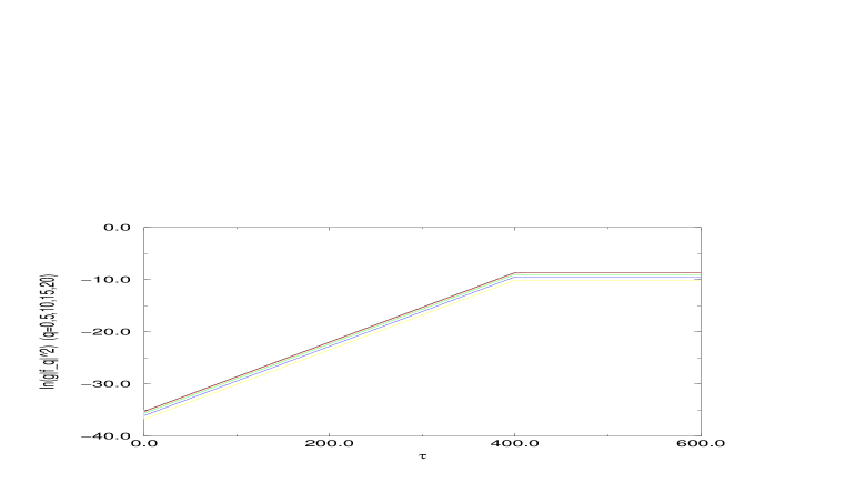
Figure 4.9: $\ln(|f_{q}(\tau)|^{2})$ vs. $\tau$, for $\eta(0)=0,\dot{\eta}(0)=0,g=10^{-14},h_{0}=10.0$ for $q=0.0,5,10,15,20$ with smaller $q$ corresponding to larger values of $\ln(|f_{q}(\tau)|^{2})$.

Figure 4.10: $p/\varepsilon$ vs. $\tau$, for $\eta(0)=0,\dot{\eta}(0)=0,g=10^{-14},h_{0}=10.0$.

4.3 Zero Mode Assembly

This remarkable feature of factorization of the mode functions after horizon crossing can be elegantly summarized as

$$f_{k}(t)|_{k_{ph}(t)\ll H_{0}}=g(q,h_{0})f_{0}(\tau),$$ (4.20)

with $k_{ph}(t)=k\,e^{-H_{0}t}$ being the physical momentum, $g(q,h_{0})$ a complex constant, and $f_{0}(\tau)$ a real function of time that satisfies the mode equation with $q=0$ and real initial conditions which will be inferred later. Since the factor $g(q,h_{0})$ depends solely on the initial conditions on the mode functions, it turns out that for two mode functions corresponding to momenta $k_{1},k_{2}$ that have crossed the horizon at times $t_{1}>t_{2}$, the ratio of the two mode functions at time $t$, ($t_{s}>t>t_{1}>t_{2}$) is

$${{f_{k_{1}}(t)}\over{f_{k_{2}}(t)}}\propto e^{(\nu-\frac{3}{2})h_{0}(\tau_{1}-\tau_{2})}>1\;.$$

Then if we consider the contribution of these modes to the renormalized quantum fluctuations a long time after the beginning of inflation (so as to neglect the decaying solutions), we find that

$$g\Sigma(\tau)\approx{\cal C}e^{(2\nu-3)h_{0}\tau}+\mbox{ small}\;,$$

where ‘small’ stands for the contribution of mode functions associated with momenta that have not yet crossed the horizon at time $\tau$, which give a perturbatively small (of order $\lambda$) contribution. We find that several e-folds after the beginning of inflation but well before inflation ends, this factorization of superhorizon modes implies the following:

$$g\int q^{2}dq\;|f^{2}_{q}(\tau)| \approx |C_{0}|^{2}f^{2}_{0}(\tau),$$ (4.21)

$$g\int q^{2}dq\;|\dot{f}^{2}_{q}(\tau)| \approx |C_{0}|^{2}\dot{f}^{2}_{0}(\tau),$$ (4.22)

$$g\int\frac{q^{4}}{a^{2}(\tau)}dq\;|f^{2}_{q}(\tau)| \approx \frac{|C_{1}|^{2}}{a^{2}(\tau)}f^{2}_{0}(\tau),$$ (4.23)

where we have neglected the weak time dependence arising from the perturbatively small contributions of the short-wavelength modes that have not yet crossed the horizon, and the integrals above are to be understood as the fully renormalized (subtracted), finite integrals. For $\eta=0$, we note that (4.21) and the fact that $f_{0}(\tau)$ obeys the equation of motion for the mode with $q=0$ leads at once to the conclusion that in this regime $\left[g\Sigma(\tau)\right]^{\frac{1}{2}}=|C_{0}|f_{0}(\tau)$ obeys the zero mode equation of motion

$$\left[\frac{d^{2}}{d\tau^{2}}+3h\frac{d}{d\tau}-1+(|C_{0}|f_{0}(\tau))^{2}\right]|C_{0}|f_{0}(\tau)=0\;.$$ (4.24)

It is clear that several e-folds after the beginning of inflation, we can define an effective zero mode as

$$\eta^{2}_{eff}(\tau)\equiv g\Sigma(\tau),\mbox{ or in dimensionful variables, }\phi_{eff}(t)\equiv\left[\langle\psi^{2}(\vec{x},t)\rangle_{R}\right]^{\frac{1}{2}}$$ (4.25)

Although this identification seems natural, we emphasize that it is by no means a trivial or ad-hoc statement. There are several important features that allow an unambiguous identification: i) $\left[\langle\psi^{2}(\vec{x},t)\rangle_{R}\right]$ is a fully renormalized operator product and hence finite, ii) because of the factorization of the superhorizon modes that enter in the evaluation of $\left[\langle\psi^{2}(\vec{x},t)\rangle_{R}\right]$, $\phi_{eff}(t)$ (4.25) obeys the equation of motion for the zero mode, iii) this identification is valid several e-folds after the beginning of inflation, after the transient decaying solutions have died away and the integral in $\langle\psi^{2}(\vec{x},t)\rangle$ is dominated by the modes with wavevector $k$ that have crossed the horizon at $t(k)\ll t$. Numerically we see that this identification holds throughout the dynamics except for a very few e-folds at the beginning of inflation. This factorization determines at once the initial conditions of the effective zero mode that can be extracted numerically: after the first few e-folds and long before the end of inflation we find

$$\phi_{eff}(t)\equiv\phi_{eff}(0)\;e^{(\nu-\frac{3}{2})H_{0}t}\;\;,$$ (4.26)

where we parameterized

$$\phi_{eff}(0)\equiv\frac{H_{0}}{2\pi}\;{\cal F}(H_{0}/m)$$

to make contact with the literature. As is shown in Fig. 4.11, we find numerically that ${\cal F}(H_{0}/m)\approx{\cal O}(1)$ for a large range of $0.1\leq H_{0}/m\leq 50$ and that this quantity depends on the initial conditions of the long wavelength modes.

Figure 4.11: ${\cal F}(H/m)$ vs. $H$, where ${\cal F}(H/m)$ is defined by the relation $\phi_{eff}(0)=(H/2\pi){\cal F}(H/m)$ [see Eqs. (4.25) and (4.26)].

Therefore, in summary, the effective composite zero mode obeys

$$\left[\frac{d^{2}}{d\tau^{2}}+3h\frac{d}{d\tau}-1+\eta^{2}_{eff}(\tau)\right]\eta_{eff}(\tau)=0\;;\;\dot{\eta}_{eff}(\tau=0)=(\nu-\frac{3}{2})\;\eta_{eff}(0)\;,$$ (4.27)

where $\eta_{eff}(0)\equiv{{\sqrt{\lambda_{R}/2}}\over{m_{R}}}\;\phi_{eff}(0)$ is obtained numerically for a given $h_{0}$ by fitting the intermediate time behavior of $g\Sigma(\tau)$ with the growing zero mode solution.

Furthermore, this analysis shows that in the case $\eta=0$, the renormalized energy and pressure in this regime in which the renormalized integrals are dominated by the superhorizon modes are given by

$$\varepsilon_{R}(\tau) \approx \frac{2Nm^{4}_{R}}{\lambda_{R}}\left\{\frac{1}{2}\dot{\eta}^{2}_{eff}+\frac{1}{4}\left(-1+\eta^{2}_{eff}\right)^{2}\right\},$$ (4.28)

$$(p+\varepsilon)_{R} \approx \frac{2Nm^{4}_{R}}{\lambda_{R}}\left\{\dot{\eta}^{2}_{eff}\right\},$$ (4.29)

where we have neglected the contribution proportional to $1/a^{2}(\tau)$ because it is effectively red-shifted away after just a few e-folds. We found numerically that this term is negligible after the interval of time necessary for the superhorizon modes to dominate the contribution to the integrals. Then the dynamics of the scale factor is given by

$$h^{2}(\tau)=4h^{2}_{0}\left\{\frac{1}{2}\dot{\eta}^{2}_{eff}+\frac{1}{4}\left(-1+\eta^{2}_{eff}\right)^{2}\right\}.$$ (4.30)

We have numerically evolved the set of effective equations (4.27, 4.30) by extracting the initial condition for the effective zero mode from the intermediate time behavior of $g\Sigma(\tau)$, and found a remarkable agreement between the evolution of $\eta^{2}_{eff}$ and $g\Sigma(\tau)$ and between the dynamics of the scale factor in terms of the evolution of $\eta_{eff}(\tau)$, and the full dynamics of the scale factor and quantum fluctuations within our numerical accuracy. Figs. 4.12 and 4.13 show the evolution of $\eta^{2}_{eff}(\tau)$ and $h(\tau)$ respectively from the classical evolution equations (4.27) and (4.30) using the initial condition $\eta_{eff}(0)$ extracted from the exponential fit of $g\Sigma(\tau)$ in the intermediate regime. These figures should be compared to Figs. 4.2 and 4.3. We have also numerically compared $p/\varepsilon$ given solely by the dynamics of the effective zero mode and it is again numerically indistinguishable from that obtained with the full evolution of the mode functions.

Figure 4.12: $\eta_{eff}^{2}(\tau)$ vs. $\tau$, for $\eta_{eff}(0)=3.94\times 10^{-7},\dot{\eta}_{eff}(0)=0.317\eta_{eff}(0),g=10^{-14},h_{0}=2.0$. The initial conditions were obtained by fitting the intermediate time regime of $g\Sigma(\tau)$ in fig. (4.2). $\eta_{eff}(\tau)$ is the solution of Eq. (4.27) with these initial conditions.

Figure 4.13: $h(\tau)$ vs. $\tau$, obtained from the solution of eqns. (4.27) and (4.30) with the conditions of fig. (4.12)).

This is one of the main results of our work. In summary: the modes that become superhorizon sized and grow through the spinodal instabilities assemble themselves into an effective composite zero mode a few e-folds after the beginning of inflation. This effective zero mode drives the dynamics of the FRW scale factor, terminating inflation when the non-linearities become important. In terms of the underlying fluctuations, the spinodal growth of superhorizon modes gives a non-perturbatively large contribution to the energy momentum tensor that drives the dynamics of the scale factor. Inflation terminates when the root mean square fluctuation probes the equilibrium minima of the tree level potential.

This phenomenon of zero mode assembly, i.e. the ‘classicalization’ of quantum mechanical fluctuations that grow after horizon crossing is very similar to the interpretation of ‘decoherence without decoherence’ of Starobinsky and Polarski[82].

The extension of this analysis to the case for which $\eta(0)\neq 0$ is straightforward. Since both $\eta(\tau)$ and $\sqrt{g\Sigma(\tau)}=|C_{0}|f_{0}(\tau)$ obey the equation for the zero mode, Eq. (4.4), it is clear that we can generalize our definition of the effective zero mode to be

$$\eta_{eff}(\tau)\equiv\sqrt{\eta^{2}(\tau)+g\Sigma(\tau)}\;.$$ (4.31)

which obeys the equation of motion of a classical zero mode:

$$\left[\frac{d^{2}}{d\tau^{2}}+3h\frac{d}{d\tau}-1+\eta_{eff}(\tau)^{2}\right]\eta_{eff}(\tau)=0\;.$$ (4.32)

If this effective zero mode is to drive the FRW expansion, then the additional condition

$$\dot{\eta}^{2}f_{0}^{2}-2\eta\dot{\eta}f_{0}\dot{f_{0}}+\eta^{2}\dot{f_{0}}^{2}=0$$ (4.33)

must also be satisfied, which is simply the condition that the contribution of the kinetic term in the effective theory is the same as that in the full theory. One can easily show that this relation is indeed satisfied if the mode functions factorize as in (4.20) and if the integrals (4.21) – (4.23) are dominated by the contributions of the superhorizon mode functions. This leads to the conclusion that the gravitational dynamics is given by eqns. (4.28) – (4.30) with $\eta_{eff}(\tau)$ defined by (4.31).

We see that in all cases, the full large $N$ quantum dynamics in these models of inflationary phase transitions is well approximated by the equivalent dynamics of a homogeneous, classical scalar field with initial conditions on the effective field $\eta_{eff}(0)\geq\sqrt{g}h_{0}{\cal F}(h_{0})$. We have verified these results numerically for the field and scale factor dynamics, finding that the effective classical dynamics reproduces the results of the full dynamics to within our numerical accuracy. We have also checked numerically that the estimate for the classical to quantum crossover given by Eq. (4.19) is quantitatively correct. Thus in the classical case in which $\eta(0)\gg\sqrt{\lambda}\;h_{0}$ we find that $\eta_{eff}(\tau)=\eta(\tau)$, whereas in the opposite, quantum case $\eta_{eff}(\tau)=\sqrt{g\Sigma(\tau)}$.

This remarkable feature of zero mode assembly of long-wavelength, spinodally unstable modes is a consequence of the presence of the horizon. It also explains why, despite the fact that asymptotically the fluctuations sample the broken symmetry state, the equation of state is that of matter. Since the excitations in the broken symmetry state are massless Goldstone bosons one would expect radiation domination. However, the assembly phenomenon, i.e. the redshifting of the wave vectors, makes these modes behave exactly like zero momentum modes that give an equation of state of matter (upon averaging over the small oscillations around the minimum).

Sub-horizon modes at the end of inflation with $q>h_{0}\,e^{h_{0}\tau_{s}}$ do not participate in the zero mode assembly. The behavior of such modes do depend on $q$ after the end of inflation. Notice that these modes have extremely large comoving $q$ since $h_{0}\,e^{h_{0}\tau_{s}}\geq 10^{26}$. As discussed in Ref. [29] such modes decrease with time after inflation as $\sim 1/a(\tau)$.

Making sense of the fluctuations

Having recognized the effective classical variable that can be interpreted as the component of the field that drives the FRW background and rolls down the classical potential hill, we want to recognize unambiguously the small fluctuations. We have argued above that after horizon crossing, all of the mode functions evolve proportionally to the zero mode, and the question arises: which modes are assembled into the effective zero mode whose dynamics drives the evolution of the FRW scale factor and which modes are treated as perturbations? In principle every $k\neq 0$ mode provides some spatial inhomogeneity, and assembling these into an effective homogeneous zero mode seems in principle to do away with the very inhomogeneities that one wants to study. However, scales of cosmological importance today first crossed the horizon during the last 60 or so e-folds of inflation. Recently Grishchuk[83] has argued that the sensitivity of the measurements of $\Delta T/T$ probe inhomogeneities on scales $\approx 500$ times the size of the present horizon. Therefore scales that are larger than these and that have first crossed the horizon much earlier than the last 60 e-folds of inflation are unobservable today and can be treated as an effective homogeneous component, whereas the scales that can be probed experimentally via the CMB inhomogeneities today must be treated separately as part of the inhomogeneous perturbations of the CMB.

Thus a consistent description of the dynamics in terms of an effective zero mode plus ‘small’ quantum fluctuations can be given provided the following requirements are met: a) the total number of e-folds $N_{e}\gg 60$, b) all the modes that have crossed the horizon before the last 60-65 e-folds are assembled into an effective classical zero mode via $\phi_{eff}(t)=\left[\phi^{2}_{0}(t)+\langle\psi^{2}(\vec{x},t)\rangle_{R}\right]^{\frac{1}{2}}$, c) the modes that cross the horizon during the last 60–65 e-folds are accounted as ‘small’ perturbations. The reason for the requirement a) is that in the separation $\phi(\vec{x},t)=\phi_{eff}(t)+\delta\phi(\vec{x},t)$ one requires that $\delta\phi(\vec{x},t)/\phi_{eff}(t)\ll 1$. As argued above, after the modes cross the horizon, the ratio of amplitudes of the mode functions remains constant and given by $e^{(\nu-\frac{3}{2})\Delta N}$ with $\Delta N$ being the number of e-folds between the crossing of the smaller $k$ and the crossing of the larger $k$. Then for $\delta\phi(\vec{x},t)$ to be much smaller than the effective zero mode, it must be that the Fourier components of $\delta\phi$ correspond to very large $k$’s at the beginning of inflation, so that the effective zero mode can grow for a long time before the components of $\delta\phi$ begin to grow under the spinodal instabilities. In fact requirement a) is not very severe; in Figs. 4.2–4.6 we have taken $h_{0}=2.0$ which is a very moderate value and yet for $\lambda=10^{-12}$ the inflationary stage lasts for well over 100 e-folds, and as argued above, the larger $h_{0}$ for fixed $\lambda$, the longer is the inflationary stage. Therefore under this set of conditions, the classical dynamics of the effective zero mode $\phi_{eff}(t)$ drives the FRW background, whereas the inhomogeneous fluctuations $\delta\phi(\vec{x},t)$, which are made up of Fourier components with wavelengths that are much smaller than the horizon at the beginning of inflation and that cross the horizon during the last 60 e-folds, provide the inhomogeneities that seed density perturbations.

4.4 Scalar Metric Perturbations

Having identified the effective zero mode and the ‘small perturbations’, we are now in position to provide an estimate for the amplitude and spectrum of scalar metric perturbations. We use the formulation by Mukhanov, Feldman and Brandenberger[45], a short review of which was provided in Sec. 2.5.

We are interested in determining the dynamics of $\Phi_{k}$ for those wavevectors that cross the horizon during the last 60 e-folds before the end of inflation. During the inflationary stage the numerical analysis yields, to a very good approximation

$$H(t)\approx H_{0}\;;\;\phi_{eff}(t)=\phi_{eff}(0)\;e^{(\nu-\frac{3}{2})H_{0}t},$$ (4.34)

where $H_{0}$ is the value of the Hubble constant during inflation, leading to

$$\Phi_{k}(t)=e^{(\nu-2)H_{0}t}\left[a_{k}\;H^{(1)}_{\beta}\left(\frac{ke^{-H_{0}t}}{H_{0}}\right)+b_{k}\;H^{(2)}_{\beta}\left(\frac{ke^{-H_{0}t}}{H_{0}}\right)\right]\;;\;\beta=\nu-1\;.$$ (4.35)

The coefficients $a_{k}$ and $b_{k}$ are determined by the initial conditions.

Since we are interested in the wavevectors that cross the horizon during the last 60 e-folds, the consistency for the zero mode assembly and the interpretation of ‘small perturbations’ requires that there must be many e-folds before the last 60. We are then considering wavevectors that were deep inside the horizon at the onset of inflation. Mukhanov et. al.[45] show that $\Phi_{k}(t)$ is related to the canonical ‘velocity field’ that determines scalar perturbations of the metric and which is quantized with Bunch-Davies initial conditions for the large $k$-mode functions. The relation between $\Phi_{k}$ and $v$ and the initial conditions on $v$ lead at once to a determination of the coefficients $a_{k}$ and $b_{k}$ for $k>>H_{0}$[45]

$$a_{k}=-\frac{3}{2}\left[\frac{8\pi}{3M^{2}_{Pl}}\right]\dot{\phi}_{eff}(0)\sqrt{\frac{\pi}{2H_{0}}}\frac{1}{k}\quad;\quad b_{k}=0\;.$$ (4.36)

Thus we find that the amplitude of scalar metric perturbations after horizon crossing is given by

$$|\delta_{k}(t)|=k^{\frac{3}{2}}|\Phi_{k}(t)|\approx\frac{3}{2}\left[\frac{8\sqrt{\pi}}{3M^{2}_{Pl}}\right]\dot{\phi}_{eff}(0)\left(\frac{2H_{0}}{k}\right)^{\nu-\frac{3}{2}}e^{(2\nu-3)H_{0}t}\;.$$ (4.37)

The time dependence of $|\delta_{k}(t)|$ displays the unstable growth associated with the spinodal instabilities of superhorizon modes and is a hallmark of the phase transition. This time dependence can be understood from the constraint equation (2.42) that relates the Bardeen potential to the gauge invariant field fluctuations[45], which in longitudinal gauge are identified with $\delta\phi(\vec{x},t)$.

Since the right hand side of (2.42) is proportional to $\dot{\phi}_{eff}/M^{2}_{Pl}\ll 1$ during the inflationary epoch in this model, we can neglect the terms proportional to $\dot{\Phi}_{k}$ and $\Phi_{k}$ on the left hand side of (2.43), in which case the equation for the gauge invariant scalar field fluctuation is the same as for the mode functions. In fact, since $\delta\phi^{gi}_{k}$ is gauge invariant we can evaluate it in the longitudinal gauge wherein it is identified with the mode functions $f_{k}(t)$. Then, absorbing a constant of integration in the initial conditions for the Bardeen variable, we find

$$\Phi_{k}(t)\approx\frac{4\pi}{M^{2}_{Pl}a(t)}\int_{t_{o}}^{t}a(t^{\prime})\;\phi_{eff}(t^{\prime})\;f_{k}(t^{\prime})\;dt^{\prime}+{\cal O}\left(\frac{1}{M^{4}_{Pl}}\right),$$ (4.38)

and using that $\phi(t)\propto e^{(\nu-3/2)H_{0}t}$ and that after horizon crossing $f_{k}(t)\propto e^{(\nu-3/2)H_{0}t}$, one obtains at once the time dependence of the Bardeen variable after horizon crossing. In particular the time dependence is found to be $\propto e^{(2\nu-3)H_{0}t}$. It is then clear that the time dependence is a reflection of the spinodal (unstable) growth of the superhorizon field fluctuations.

To obtain the amplitude and spectrum of density perturbations at second horizon crossing we use the conservation law, Eq. (2.44), which is valid after horizon crossing of the mode with wavevector $k$. Although this conservation law is an exact statement of superhorizon mode solutions of Eq. (2.41), we have obtained solutions assuming that during the inflationary stage $H$ is constant and have neglected the $\dot{H}$ term in Eq. (2.41). Since during the inflationary stage,

$$\dot{H}(t)=-\frac{4\pi}{M^{2}_{Pl}}\,\dot{\phi}^{2}_{eff}(t)\propto H^{2}_{0}\;\left(\frac{d\eta_{eff}(\tau)}{d\tau}\right)^{2}\ll H^{2}_{0}$$ (4.39)

and $\ddot{\phi}/\dot{\phi}\approx H_{0}$, the above approximation is justified. We then see that $\phi^{2}_{eff}(t)\propto e^{(2\nu-3)H_{0}t}$ which is the same time dependence as that of $\Phi_{k}(t)$. Thus the term proportional to $1/(1+p/\varepsilon)$ in Eq. (2.44) is indeed constant in time after horizon crossing. On the other hand, the term that does not have this denominator evolves in time but is of order $(1+p/\varepsilon)=-2\dot{H}/3H^{2}\ll 1$ with respect to the constant term and therefore can be neglected. Thus, we confirm that the variable $\xi$ is conserved up to the small term proportional to $(1+p/\varepsilon)\Phi_{k}$ which is negligible during the inflationary stage. This small time dependence is consistent with the fact that we neglected the $\dot{H}$ term in the equation of motion for $\Phi_{k}(t)$.

However, upon second horizon crossing it is straightforward to see that $\dot{\Phi}_{k}(t_{f})\approx 0$. The reason for this assertion can be seen as follows: Eq. (2.43) shows that at long times, when the effective zero mode is oscillating around the minimum of the potential with a very small amplitude and when the time dependence of the fluctuations has saturated (see Fig. 4.4), $\Phi_{k}$ will redshift as $\approx 1/a(t)$[29] and its derivative becomes extremely small.

Using this conservation law, assuming matter domination at second horizon crossing, and $\dot{\Phi}_{k}(t_{f})\approx 0$[45], we find

$$|\delta_{k}(t_{f})|=\frac{12\,\Gamma(\nu)\,\sqrt{\pi}}{5\,(\nu-\frac{3}{2})\,{\cal F}(H_{0}/m)}\left(\frac{2H_{0}}{k}\right)^{\nu-\frac{3}{2}},$$ (4.40)

where ${\cal F}(H_{0}/m)$ determines the initial amplitude of the effective zero mode (4.26). We can now read the power spectrum per logarithmic $k$ interval

$${\cal P}_{s}(k)=|\delta_{k}|^{2}\propto k^{-2(\nu-\frac{3}{2})}\equiv k^{n_{s}-1}\;.$$ (4.41)

leading to the index for scalar density perturbations

$$n_{s}=1-2\left(\nu-\frac{3}{2}\right)\;.$$ (4.42)

For $H_{0}/m\gg 1$, we can expand $\nu-3/2$ as a series in $m^{2}/H_{0}^{2}$ in Eq. (4.40). Given that the comoving wavenumber of the mode which crosses the horizon $n$ $e$-folds before the end of inflation is $k=H_{0}e^{(N_{e}-n)}$ where $N_{e}$ is given by (4.16), we arrive at the following expression for the amplitude of fluctuations on the scale corresponding to $n$ in terms of the De Sitter Hubble constant and the coupling $\lambda$:

$$|\delta_{n}(t_{f})|\simeq\frac{9H_{0}^{3}}{5\sqrt{2}m^{3}}\left(2e^{n}\right)^{m^{2}/3H_{0}^{2}}\sqrt{\lambda}\left[1+\frac{2m^{2}}{3H_{0}^{2}}\left(\frac{7}{6}-\ln 2-\frac{\gamma}{2}\right)+{\cal O}\left(\frac{m^{4}}{H_{0}^{4}}\right)\right]\;.$$ (4.43)

Here, $\gamma$ is Euler’s constant. Note the explicit dependence of the amplitude of density perturbations on $\sqrt{\lambda}$. For $n\approx 60$, the factor $\exp(nm^{2}/3H_{0}^{2})$ is ${\cal O}(100)$ for $H_{0}/m=2$, while it is ${\cal O}(1)$ for $H_{0}/m\geq 4$. Notice that for $H_{0}/m$ large, the amplitude increases approximately as $(H_{0}/m)^{3}$, which will place strong restrictions on $\lambda$ in such models.

We remark that we have not included the small corrections to the dynamics of the effective zero mode and the scale factor arising from the non-linearities. We have found numerically that these nonlinearities are only significant for the modes that cross about 60 $e$-folds before the end of inflation for values of the Hubble parameter $H_{0}/m_{R}>5$. The effect of these non-linearities in the large $N$ limit is to slow somewhat the exponential growth of these modes, with the result of shifting the power spectrum closer to an exact Harrison-Zeldovich spectrum with $n_{s}=1$. Since for $H_{0}/m_{R}>5$ the power spectrum given by (4.42) differs from one by at most a few percent, the effects of the non-linearities are expected to be observationally unimportant. The spectrum given by (4.40) is similar to that obtained in references[21, 13] although the amplitude differs from that obtained there. In addition, we do not assume slow roll for which $(\nu-\frac{3}{2})\ll 1$, although this would be the case if $N_{e}\gg 60$.

We emphasize an important feature of the spectrum: it has more power at long wavelengths because $\nu-3/2>0$. This is recognized to be a consequence of the spinodal instabilities that result in the growth of long wavelength modes and therefore in more power for these modes. This seems to be a robust prediction of new inflationary scenarios in which the potential has negative second derivative in the region of field space that produces inflation.

It is at this stage that we recognize the consistency of our approach for separating the composite effective zero mode from the small fluctuations. We have argued above that many more than 60 $e$-folds are required for consistency, and that the small fluctuations correspond to those modes that cross the horizon during the last 60 $e$-folds of the inflationary stage. For these modes $H_{0}/k=e^{-H_{0}t^{*}(k)}$ where $t^{*}(k)$ is the time since the beginning of inflation of horizon crossing of the mode with wavevector $k$. The scale that corresponds to the Hubble radius today $\lambda_{0}=2\pi/k_{0}$ is the first to cross during the last 60 or so $e$-folds before the end of inflation. Smaller scales today will correspond to $k>k_{0}$ at the onset of inflation since they will cross the first horizon later and therefore will reenter earlier. The bound on $|\delta_{k_{0}}|\propto\Delta T/T\leq 10^{-5}$ on these scales provides a lower bound on the number of $e$-folds required for these type of models to be consistent:

$$N_{e}>60+\frac{12}{\nu-\frac{3}{2}}-\frac{\ln(\nu-\frac{3}{2})}{\nu-\frac{3}{2}}\;,$$ (4.44)

where we have written the total number of $e$-folds as $N_{e}=H_{0}\;t^{*}(k_{0})+60$. This in turn can be translated into a bound on the coupling constant using the estimate given by Eq. (4.16).

Since the COBE satellite observes microwave background temperature variation with a resolution of a single degree or larger, which is approximately the size of the particle horizon at the time of recombination, we may directly compare the power spectrum for thermal fluctuations measured by COBE with the spectrum computed here for fluctuations at second horizon crossing [see Eq. (2.40)]. The four year COBE DMR Sky Map[85] gives $n\approx 1.2\pm 0.3$ thus providing an upper bound on $\nu$

$$0\leq\nu-\frac{3}{2}\leq 0.05$$ (4.45)

corresponding to $h_{0}\geq 2.6$. We then find that these values of $h_{0}$ and $\lambda\approx 10^{-12}-10^{-14}$ provide sufficient $e$-folds to satisfy the constraint for scalar density perturbations.

4.5 Decoherence: Quantum to Classical Transition During Inflation

An important aspect of cosmological perturbations is that they are of quantum origin but eventually they become classical as they are responsible for the small classical metric perturbations. This quantum to classical crossover is associated with a decoherence process and has received much attention[82, 84].

Recent work on decoherence focused on the description of the evolution of the density matrix for a free scalar massless field that represents the “velocity field”[45] associated with scalar density perturbations[82]. In this section we study the quantum to classical transition of superhorizon modes for the Bardeen variable by relating these to the field mode functions and analyzing the full time evolution of the density matrix of the matter field. This is accomplished with the identification given by equation (4.38) which relates the mode functions of the Bardeen variable with those of the scalar field. This relation establishes that in the models under consideration the classicality of the Bardeen variable is determined by the classicality of the scalar field modes.

In the situation under consideration, long-wavelength field modes become spinodally unstable and grow exponentially after horizon crossing. The factorization (4.14) results in the phases of these modes “freezing out”. This feature and the growth in amplitude entail that these modes become classical. The relation (4.38) in turn implies that these features also apply to the superhorizon modes of the Bardeen potential.

Therefore we can address the quantum to classical transition of the Bardeen variable (gravitational potential) by analyzing the evolution of the density matrix for the matter field.

To make contact with previous work[82, 84] we choose to study the evolution of the field density matrix in conformal time (see Sec. 2.4), although the same features will be displayed in comoving time. Note that we use $\eta$ to denote conformal time throughout this section; it should not be confused with the dimensionless, comoving time zero mode $\eta(t)$.

The conformal time Hamiltonian operator, which is the generator of translations in $\eta$, is given by

$$H_{\eta}=\int d^{3}x\left\{\frac{1}{2}\Pi^{2}_{\vec{\chi}}+\frac{1}{2}(\vec{\nabla}\vec{\chi})^{2}+{\cal{V}}(\vec{\chi})\right\},$$ (4.46)

with $\vec{\Pi}_{\chi}$ being the canonical momentum conjugate to $\vec{\chi}$, $\vec{\Pi}_{\chi}=\vec{\chi}^{\prime}$. Separating the zero mode of the field $\vec{\chi}$

$$\vec{\chi}(\vec{x},\eta)=\chi_{0}(\eta)\delta_{i,1}+{\hat{\vec{\chi}}}(\vec{x},\eta),$$ (4.47)

and performing the large $N$ factorization on the fluctuations we find that the Hamiltonian becomes linear plus quadratic in the fluctuations, and similar to a Minkowski space-time Hamiltonian with a $\eta$ dependent mass term given by

$${\cal{M}}^{2}(\eta)=a^{2}(\eta)\left[m^{2}+\left(\xi-\frac{1}{6}\right)\,{\cal{R}}+\frac{\lambda}{2}\,\chi_{0}^{2}(\eta)+\frac{\lambda}{2}\,\langle\hat{\chi}^{2}\rangle\right].$$ (4.48)

We can now follow the steps and use the results of ref.[26] for the conformal time evolution of the density matrix by setting $a(t)=1$ in the proper equations of that reference and replacing the frequencies by

$$\omega^{2}_{k}(\eta)=\vec{k}^{2}+{\cal{M}}^{2}(\eta)\;.$$ (4.49)

The expectation value in Eq. (4.48) and that of the energy momentum tensor are obtained in this $\eta$ evolved density matrix. [As is clear, we obtain in this way the self-consistent dynamics in the curved cosmological background (2.29)].

The time evolution of the kernels in the density matrix (see [26]) is determined by the mode functions that obey

$$\left[\frac{d^{2}}{d\eta^{2}}+k^{2}+{\cal{M}}^{2}(\eta)\right]F_{k}(\eta)=0.$$ (4.50)

The Wronskian of these mode functions

$${\cal{W}}(F,F^{*})=F^{\prime}_{k}F^{*}_{k}-F_{k}F^{\prime*}_{k}$$ (4.51)

is a constant. It is natural to impose initial conditions such that at the initial $\eta$ the density matrix describes a pure state which is the instantaneous ground state of the Hamiltonian at this initial time. This implies that the initial conditions of the mode functions $F_{k}(\eta)$ be chosen to be (see [26])

$$F_{k}(\eta_{o})=\frac{1}{\sqrt{\omega_{k}(\eta_{o})}}\;\;;\;F^{\prime}_{k}(\eta_{o})=-i\omega_{k}(\eta_{o})\;F_{k}(\eta_{o}).$$ (4.52)

With such initial conditions, the Wronskian (4.51) takes the value

$${\cal{W}}(F,F^{*})=-2i\;.$$ (4.53)

The Heisenberg field operators $\hat{\chi}(\vec{x},\eta)$ and their canonical momenta $\Pi_{\chi}(\vec{x},\eta)$ can now be expanded as:

$$\hat{\vec{\chi}}(\vec{x},\eta)=\int{{d^{3}k}\over{(2\pi)^{3/2}}}\left[\vec{a}_{\vec{k}}\;F_{k}(\eta)+\vec{a}^{\dagger}_{-\vec{k}}\;F^{*}_{k}(\eta)\right]e^{i\vec{k}\cdot\vec{x}},$$ (4.54)

$$\vec{\Pi}_{\chi}(\vec{x},\eta)=\int{{d^{3}k}\over{(2\pi)^{3/2}}}\left[\vec{a}_{\vec{k}}\;F^{\prime}_{k}(\eta)+\vec{a}^{\dagger}_{-\vec{k}}\;F^{\prime*}_{k}(\eta)\right]e^{i\vec{k}\cdot\vec{x}},$$ (4.55)

with the time independent creation and annihilation operators $\vec{a}_{\vec{k}}$ and $\vec{a}^{\dagger}_{\vec{k}}$ obeying canonical commutation relations. Since the fluctuation fields in comoving and conformal time are related by a conformal rescaling given by Eq. (2.30) it is straightforward to see that the mode functions in comoving time $t$ are related to those in conformal time simply as

$$f_{k}(t)=\frac{F_{k}(\eta)}{a(\eta)}.$$ (4.56)

Therefore the initial conditions given in Eq. (4.52) on the conformal time mode functions and the choice $a(t_{0})=a(\eta_{0})=1$ imply the initial conditions for the mode functions in comoving time given by Eq. (3.92).

In conformal time, the density matrix takes the form

$$\rho[\Phi,\tilde{\Phi},\eta] = \prod_{\vec{k}}{\cal{N}}_{k}(\eta)\exp\left\{-\frac{1}{2}A_{k}(\eta)\;\vec{\eta}_{\vec{k}}(\eta)\cdot\vec{\eta}_{-{\vec{k}}}(\eta)-\frac{1}{2}A^{*}_{k}(\eta)\;\tilde{\vec{\eta}}_{\vec{k}}(\eta)\cdot\tilde{\vec{\eta}}_{-{\vec{k}}}(\eta)\right.$$ (4.57)

$$\left.-\;B_{k}(\eta)\;\vec{\eta}_{\vec{k}}({\cal T})\cdot\tilde{\vec{\eta}}_{-{\vec{k}}}(\eta)+i\,\vec{\pi}_{\vec{k}}(\eta)\cdot\left(\vec{\eta}_{-{\vec{k}}}(\eta)-\tilde{\vec{\eta}}_{-{\vec{k}}}(\eta)\right)\right\};\ ,$$

$$\vec{\eta}_{\vec{k}}(\eta) = \vec{\chi}_{\vec{k}}(\eta)-\chi_{0}(\eta)\,\delta_{i,1}\;\delta(\vec{k})\;\;;\;\;\tilde{\vec{\eta}}_{k}(\eta)={\tilde{\vec{\chi}}}_{k}(\eta)-\chi_{0}(\eta)\,\delta_{i,1}\;\delta(\vec{k})\;.$$

$\vec{\pi}_{\vec{k}}(\eta)$ is the Fourier transform of $\Pi_{\chi}(\eta,\vec{x})$.

In conformal time quantization and in the Schrödinger representation in which the field $\chi$ is diagonal the conformal time evolution of the density matrix is via the conformal time Hamiltonian (4.46). The evolution equations for the covariances are obtained from those given in ref.[26] by setting $a(t)=1$ and using the frequencies $\omega^{2}_{k}(\eta)=k^{2}+{\cal{M}}^{2}(\eta)$. In particular, by setting the covariance of the diagonal elements (given by equation (2.20) in [26]; see also equation (2.44) of [26]),

$$A_{k}(\eta)=-i\,\frac{F^{\prime*}_{k}(\eta)}{F^{*}_{k}(\eta)}.$$ (4.58)

More explicitly [26],

$${\cal{N}}_{k}(\eta) = {\cal{N}}_{k}(\eta_{0})\;\exp\left[\int_{\eta_{0}}^{\eta}A_{Ik}(\eta^{\prime})\;d\eta^{\prime}\right]={{{\cal N}_{k}(\eta_{0})}\over{\sqrt{\omega_{k}(\eta_{o})}\;|F_{k}(\eta)|}}\;,$$ (4.59)

$$A_{Ik}(\eta) = -{d\over{d\eta}}\log|F_{k}(\eta)|=-{\dot{a}}(t)-a(t)\;{d\over{dt}}\log|f_{k}(t)|\;,$$ (4.61)

$$A_{Rk}(\eta) = {1\over{|F_{k}(\eta)|^{2}}}\,={1\over{a(t)^{2}\;|f_{k}(t)|^{2}}}\;,$$ (4.63)

$$B_{k}(\eta) \equiv 0\;,$$

where $A_{Rk}$ and $A_{Ik}$ are respectively the real and imaginary parts of $A_{k}$ and we have used the value of the Wronskian (4.53) in evaluating (4.59).

The coefficients $A_{k}(\eta)$ and ${\cal{N}}_{k}(\eta)$ in the Gaussian density matrix (4.57) are completely determined by the conformal mode functions $F_{k}(\eta)$ [or alternatively the comoving time mode functions $f_{k}(t)$].

Let us study the time behavior of these coefficients. During inflation, $a(t)\approx e^{h_{0}t}$, and the mode functions factorize after horizon crossing. Further, superhorizon modes grow in cosmic time as in Eq. (4.14):

$$a^{2}(t)|f_{k}(t)|^{2}\approx{1\over{\cal D}_{k}}\;e^{(2\nu-1)h_{0}t}$$

where the coefficient ${\cal D}_{k}$ can be read from Eq. (4.14).

We emphasize that this is a result of the full evolution as displayed from the numerical solution in Fig. 4.4. These mode functions encode all of the self-consistent and non-perturbative features of the dynamics. This should be contrasted with other studies in which typically free field modes in a background metric are used.

Inserting this expression in Eqs. (4.59) yields

$$A_{Ik}(\eta) \buildrel t\to\infty\over{=} -h_{0}\;e^{h_{0}t}\left(\nu-\frac{1}{2}\right)+{\cal O}(e^{-h_{0}t})\;,$$ (4.65)

$$A_{Rk}(\eta) \buildrel t\to\infty\over{=} {\cal D}_{k}\;\;e^{-(2\nu-1)h_{0}t}.$$

Since $\nu-\frac{1}{2}>1$, we see that the imaginary part of the covariance $A_{Ik}(\eta)$ grows very fast. Hence, the off-diagonal elements of $\rho[\Phi,\tilde{\Phi},\eta]$ oscillate wildly after a few $e$-folds of inflation. In particular their contribution to expectation values of operators will be washed out. That is, we quickly reach a classical regime where only the diagonal part of the density matrix is relevant:

$$\rho[\Phi,\Phi,\eta]=\prod_{\vec{k}}{\cal{N}}_{k}(\eta)\exp\left\{-A_{Rk}(\eta)\;\eta_{\vec{k}}(\eta)\;{\eta}_{-{\vec{k}}}(\eta)\right\}.$$ (4.67)

The real part of the covariance $A_{Rk}(\eta)$ (as well as any non-zero mixing kernel $B_{k}(\eta)$[26]) decreases as $e^{-(2\nu-1)h_{0}t}$. Therefore, characteristic field configurations $\eta_{\vec{k}}$ are very large (of order $e^{(\nu-\frac{1}{2})h_{0}t}$). Therefore configurations with field amplitudes up to ${\cal O}(e^{(\nu-\frac{1}{2})h_{0}t})$ will have a substantial probability of occurring and being represented in the density matrix.

Notice that $\chi\sim e^{(\nu-\frac{1}{2})h_{0}t}$ corresponds to field configurations $\Phi$ with amplitudes of order $e^{(\nu-\frac{3}{2})h_{0}t}$ [see Eq. (2.30)]. It is the fact that $\nu-\frac{3}{2}>0$ which in this situation is responsible for the “classicalization”, which is seen to be a consequence of the spinodal growth of long-wavelength fluctuations.

The equal-time field correlator is given by

$$\langle\bar{\chi}(\vec{x},\eta)\;\bar{\chi}({\vec{x}}^{\prime},\eta)\rangle = \int\frac{d^{3}k}{2(2\pi)^{3}}\;|F_{k}(\eta)|^{2}\;e^{i{\vec{k}}.({\vec{x}}-{\vec{x}}^{\prime})}\quad,$$ (4.68)

$$= a(t)^{2}\;\int\frac{d^{3}k}{2(2\pi)^{3}}\;|f_{k}(t)|^{2}\;e^{i{\vec{k}}.({\vec{x}}-{\vec{x}}^{\prime})}\quad.$$ (4.70)

and is seen to be dominated by the superhorizon mode functions and to grow as $e^{(2\nu-1)h_{0}t}$, whereas the field commutators remain fixed showing the emergence of a classical behavior. As a result we obtain

$$\langle\bar{\chi}(\vec{x},\eta)\;\bar{\chi}({\vec{x}}^{\prime},\eta)\rangle\propto a^{2}(t)\;\phi_{eff}(t)\;\phi_{eff}(t^{\prime})\;G(|\vec{x}-\vec{x}^{\prime}|)+\mbox{ small }$$ (4.71)

where $G(|\vec{x}-\vec{x}^{\prime}|)$ falls off exponentially for distances larger than the horizon[27] and “small” refers to terms that are smaller in magnitude. This factorization of the correlation functions is another indication of classicality.

Therefore, it is possible to describe the physics by using classical field theory. More precisely, one can use a classical statistical (or stochastic) field theory described by the functional probability distribution (4.67).

These results generalize the decoherence treatment given in ref.[82] for a free massless field in pure quantum states to the case of interacting fields with broken symmetry. Note that the formal decoherence or classicalization in the density matrix appears after the modes with wave vector $k$ become superhorizon sized i.e. when the factorization of the mode functions becomes effective.

4.6 Conclusions

It can be argued that the inflationary paradigm as currently understood is one of the greatest applications of quantum field theory. The imprint of quantum mechanics is everywhere, from the dynamics of the inflaton, to the generation of metric perturbations, through to the reheating of the universe. It is clear then that we need to understand the quantum mechanics of inflation in as deep a manner as possible so as to be able to understand what we are actually testing via the CBR temperature anisotropies.

What we have found in our work is that the quantum mechanics of inflation is extremely subtle. We now understand that it involves both non-equilibrium as well as non-perturbative dynamics and that what you start from may not be what you wind up with at the end.

In particular, we see now that the correct interpretation of the non-perturbative growth of quantum fluctuations via spinodal decomposition is that the background zero mode must be redefined through the process of zero mode reassembly. When this is done we can interpret inflation in terms of the usual slow-roll approach with the now small quantum fluctuations around the redefined zero mode driving the generation of metric perturbations.

We have studied the non-equilibrium dynamics of a ‘new inflation’ scenario in a self-consistent, non-perturbative framework based on a large $N$ expansion, including the dynamics of the scale factor and backreaction of quantum fluctuations. Quantum fluctuations associated with superhorizon modes grow exponentially as a result of the spinodal instabilities and contribute to the energy momentum tensor in such a way as to end inflation consistently.

Analytical and numerical estimates have been provided that establish the regime of validity of the classical approach. We find that these superhorizon modes re-assemble into an effective zero mode and unambiguously identify the composite field that can be used as an effective expectation value of the inflaton field whose classical dynamics drives the evolution of the scale factor. This identification also provides the initial condition for this effective zero mode.

A consistent criterion is provided to extract “small” fluctuations that will contribute to cosmological perturbations from “large” non-perturbative spinodal fluctuations. This is an important ingredient for a consistent calculation and interpretation of cosmological perturbations. This criterion requires that the model must provide many more than 60 $e$-folds to identify the ‘small perturbations’ that give rise to scalar metric (curvature) perturbations. We then use this criterion combined with the gauge invariant approach to obtain the dynamics of the Bardeen variable and the spectrum for scalar perturbations.

We find that during the inflationary epoch, superhorizon modes of the Bardeen potential grow exponentially in time reflecting the spinodal instabilities. These long-wavelength instabilities are manifest in the spectrum of scalar density perturbations and result in an index that is less than one, i.e. a “red” power spectrum, providing more power at long wavelength. We argue that this ‘red’ spectrum is a robust feature of potentials that lead to spinodal instabilities in the region in field space associated with inflation and can be interpreted as an “imprint” of the phase transition on the cosmological background. Tensor perturbations on the other hand, are not modified by these features, they have much smaller amplitude and a Harrison-Zeldovich spectrum.

We made contact with the reconstruction program and validated the results for these type of models based on the slow-roll assumption, despite the fact that our study does not involve such an approximation and is non-perturbative.

Finally we have studied the quantum to classical crossover and decoherence of quantum fluctuations by studying the full evolution of the density matrix, thus making contact with the concept of “decoherence without decoherence”[82] which is generalized to the interacting case. In the case under consideration decoherence and classicalization is a consequence of spinodal growth of superhorizon modes and the presence of a horizon. The phases of the mode functions “freeze out” and the amplitudes of the superhorizon modes grow exponentially during the inflationary stage, again as a result of long-wavelength instabilities. As a result field configurations with large amplitudes have non-vanishing probabilities to be represented in the dynamical density matrix. In the situation considered, the quantum to classical crossover of cosmological perturbations is directly related to the “classicalization” of superhorizon matter field modes that grow exponentially upon horizon crossing during inflation. The diagonal elements of the density matrix in the Schroedinger representation can be interpreted as a classical distribution function, whereas the off-diagonal elements are strongly suppressed during inflation.

Chapter 5 Explosive Particle Production After Inflation

5.1 Introduction

The most popular of current models of inflation is probably the chaotic inflation models[86]. Unlike the old or new inflation models which rely on the inflaton being near some local extremum of the potential, typically with $\phi(t_{0})\ll|m|/\sqrt{\lambda}$, chaotic inflation requires initial values of the field which are large, typically with $\phi(t_{0})\gg|m|/\sqrt{\lambda}$ (see Fig. 5.1). For such large field values, the potential contribution dominates the energy momentum, leading to inflation.

Figure 5.1: A typical chaotic inflation potential. The field $\Phi$ begins at very high field values, far from the minimum.

Unlike the new inflationary scenario examined in the preceding chapter, there are no spinodal instabilities in chaotic inflation and the dynamics of the inflationary phase are relatively straightforward. In particular, during inflation, quantum fluctuations remain small and one may simply treat the inflaton as a classical field identified as the mean value of the quantum field. That is, it is safe to write $\phi_{cl}(t)=\phi(t)$ and be sure that corrections to the classical evolution remain perturbatively small.

However, as we shall see, the post inflationary evolution may not be so straightforward.

In addition to other aspects of inflation, the question of the reheating of the universe, the transfer of energy from the inflaton to other particle modes, has received much attention [42]. The reason for this is that exponential expansion during inflation causes the universe to become very cold, as the energy in fields other than the inflaton is redshifted away. In order to achieve the standard results of nucleosynthesis, and possibly other early processes, the universe must be reheated to temperatures above those at which these important processes take place. Early efforts to account for the necessary reheating introduced ad hoc decay widths to the inflaton, assuming the energy transfer occurred through single particle decay [87]. However, more recently, it has been realized that there are much more efficient processes, those of either spinodal decomposition in the case of a (new) inflationary phase transition and parametric amplification in the case of chaotic inflationary scenarios [23, 24, 25, 56, 57, 58, 59, 60, 61, 36]. Such mechanisms, in which the rate of energy transfer grows exponentially, are referred to generally as preheating.

In particular, we will study the process of preheating using a wide range of initial conditions. We analyze the dynamics of preheating in fixed radiation and matter dominated Friedmann-Robertson-Walker cosmologies both analytically and numerically.

Our main results are as follows. In the situations we analyze, we find that the expansion of the universe allows for significant particle production, although this production is somewhat sensitive to the exact expansion rate and is effectively shut off for high enough rates. In the case of a symmetry broken potential, we determine that in the large $N$ limit, the quantum fluctuations decrease for late times as $1/a^{2}(t)$, while, as in Ch. 4, these fluctuations and the zero mode satisfy a sum rule consistent with Goldstone’s theorem [see Eq. (4.6)].

We compute the renormalized energy density, $\varepsilon$, and the pressure, $p$, as a function of time. Averaging over the field oscillations, we find immediately after preheating a cold matter equation of state ($p=0$) in the slow roll scenarios. In chaotic scenarios, the equation of state just after preheating is between that of radiation ($p=\varepsilon/3$) and matter where the matter dominated regime is reached only for late times. The time scale over which the equation of state becomes matter dominated depends on the distribution of created particles in momentum space in addition to the approximation scheme implemented.

5.2 Evolution

We focus our study of the evolution on radiation or matter dominated cosmologies, as the case for de Sitter expansion has been studied previously[27]. We write the scale factor as $a(t)=(t/t_{0})^{n}$ with $n=1/2$ and $n=2/3$ corresponding to radiation and matter dominated backgrounds respectively. Note that the value of $t_{0}$ determines the initial Hubble constant since

$$H(t_{0})=\frac{\dot{a}(t_{0})}{a(t_{0})}=\frac{n}{t_{0}}.$$

We now solve the system of Eqs. (LABEL:hartphieq)–(3.91) in the Hartree approximation and in the large $N$ limit. We begin by presenting an early time analysis of the slow roll scenario. We then undertake a thorough numerical investigation of various cases of interest. For the symmetry broken case, we also provide an investigation of the late time behavior of the zero mode and the quantum fluctuations.

It will also be convenient to define the number operator $N(t)$. We do so using conformal time quantization, as the particles so defined will most closely match the definition of particles in flat spacetime[29]. We have, at zero temperature,

$$N_{k}(t)=\frac{a^{2}(t)}{4}\left|\frac{f_{k}(t)}{f_{k}(t_{0})}\right|^{2}\left[1+\frac{1}{\omega^{2}_{k}(t_{0})}\left|\frac{\dot{f}_{k}(t)+H(t)f_{k}(t)}{f_{k}(t)}\right|^{2}\right]-\frac{1}{2}\;.$$ (5.1)

Examination of the large $k$ behavior of $f_{k}$ and $\dot{f}_{k}$ shows that $N_{k}$ is ${\cal O}(1/k^{4})$ for large $k$, so that the total number of particles

$$N(t)=\int\frac{d^{3}k}{(2\pi)^{3}}N_{k}$$ (5.2)

is finite.

In what follows, we will assume minimal coupling to the curvature, $\xi_{R}=0$. In most of the cases of interest, ${\cal R}/|m|\ll 1$, so that finite $\xi_{R}$ has little effect.

5.2.1 Early Time Solutions for Slow Roll

For early times in a slow roll scenario [$m^{2}=-1$, $\eta(\tau_{0})\ll 1$], we can neglect in Eq. (LABEL:hartphieq) and in Eq. (LABEL:hartukeq) both the quadratic and cubic terms in $\phi(t)$ as well as the quantum fluctuations $\langle\psi^{2}(t)\rangle_{R}$ [recall that $\langle\psi^{2}(t_{0})\rangle_{R}=0$]. Thus, the differential equations for the zero mode (LABEL:hartphieq) and the mode functions (LABEL:hartukeq) become linear equations. In terms of the scaled variables introduced at the beginning of Sec. 4.2, with $a(\tau)=(\tau/\tau_{0})^{n}$ ($n=2/3$ for a matter dominated cosmology while $n=1/2$ for a radiation dominated cosmology) we have:

$$\ddot{\eta}(\tau)+\frac{3n}{\tau}\dot{\eta}(\tau)-\eta(\tau) = 0\;,$$ (5.3)

$$\left[\frac{d^{2}}{d\tau^{2}}+\frac{3n}{\tau}\frac{d}{d\tau}+\frac{q^{2}}{(\tau/\tau_{0})^{2n}}-1\right]f_{q}(\tau) = 0\;.$$ (5.4)

The solutions to the zero mode equation (5.3) are

$$\eta(\tau)=c\;\tau^{-\nu}I_{\nu}(\tau)+d\;\tau^{-\nu}K_{\nu}(\tau)\;,$$ (5.5)

where $\nu\equiv(3n-1)/2$, and $I_{\nu}(\tau)$ and $K_{\nu}(\tau)$ are modified Bessel functions. The coefficients, $c$ and $d$, are determined by the initial conditions on $\eta$. For $\eta(\tau_{0})=\eta_{0}$ and $\dot{\eta}(\tau_{0})=0$, we have:

$$c = \eta_{0}\;\tau_{0}^{\nu+1}\left[\dot{K}_{\nu}(\tau_{0})-\frac{\nu}{\tau_{0}}K_{\nu}(\tau_{0})\right]\;,$$ (5.6)

$$d = -\eta_{0}\;\tau_{0}^{\nu+1}\left[\dot{I}_{\nu}(\tau_{0})-\frac{\nu}{\tau_{0}}I_{\nu}(\tau_{0})\right]\;.$$ (5.7)

Taking the asymptotic forms of the modified Bessel functions, we find that for intermediate times $\eta(\tau)$ grows as

$$\eta(\tau)\stackrel{{\scriptstyle\tau\gg 1}}{{=}}{c\over{\sqrt{2\pi}}}\;\tau^{-3n/2}\;e^{\tau}\left[1-\frac{9n^{2}-6n}{8\tau}+O\left({1\over{\tau^{2}}}\right)\right].$$ (5.8)

We see that $\eta(\tau)$ grows very quickly in time, and the approximations (5.3) and (5.4) will quickly break down. For the case shown in Fig. 5.2 (with $n=2/3$, $h(\tau_{0})=0.1$, $\eta(\tau_{0})=10^{-7}$, and $\dot{\eta}(\tau_{0})=0$), we find that this approximation is valid up to $\tau-\tau_{0}\simeq 10$.

The equations for the mode functions (5.4) can be solved in closed form for the modes in the case of a radiation dominated cosmology with $n=1/2$. The solutions are

$$f_{q}(\tau)=c_{q}\;e^{-\tau}\,U\left(\frac{3}{4}-\frac{q^{2}\tau_{0}}{2},\frac{3}{2},2\tau\right)+d_{q}\;e^{-\tau}\,M\left(\frac{3}{4}-\frac{q^{2}\tau_{0}}{2},\frac{3}{2},2\tau\right).$$ (5.9)

Here, $U(\cdot)$ and $M(\cdot)$ are confluent hypergeometric functions [88] (in another common notation, $M(\cdot)\equiv\;_{1}F_{1}(\cdot)$), and the $c_{q}$ and $d_{q}$ are coefficients determined by the initial conditions (3.92) on the modes. The solutions can also be written in terms of parabolic cylinder functions.

For large $\tau$ we have the asymptotic form

$$f_{q}(\tau) \stackrel{{\scriptstyle\tau\gg 1}}{{=}} d_{q}\;e^{\tau}(2\tau)^{-(3/4+q^{2}\tau_{0}/2)}\frac{\sqrt{\pi}}{2\;\Gamma\left(\frac{3}{4}-\frac{q^{2}\tau_{0}}{2}\right)}\left[1+O\left({1\over{\tau}}\right)\right]$$ (5.10)

$$+ c_{q}\;e^{-\tau}\,(2\tau)^{(-3/4+q^{2}\tau_{0}/2)}\left[1+O\left({1\over{\tau}}\right)\right]\;.$$

Again, these expressions only apply for intermediate times before the nonlinearities have grown significantly.

5.2.2 Numerical Analysis

We now present the numerical analysis of the dynamical evolution of scalar fields in time dependent, matter and radiation dominated cosmological backgrounds. We use initial values of the Hubble constant such that $h(\tau_{0})\geq 0.1$. For expansion rates much less than this value the evolution will look similar to Minkowski space, which has been studied in great detail elsewhere [25, 54, 40]. As will be seen, the equation of state found numerically is, in the majority of cases, that of cold matter. We therefore use matter dominated expansion for the evolution in much of the analysis that follows. While it presents some inconsistency at late times, the evolution in radiation dominated universes remains largely unchanged, although there is greater initial growth of quantum fluctuations due to the scale factor growing more slowly in time. Using the large $N$ and Hartree approximations to study theories with continuous and discrete symmetries respectively, we treat three important cases. They are

1. $m^{2}<0$, $\eta(\tau_{0})\ll 1$,

2. $m^{2}<0$, $\eta(\tau_{0})\gg 1$, and

3. $m^{2}>0$, $\eta(\tau_{0})\gg 1$.

In presenting the figures, we have shifted the origin of time such that $\tau\to\tau^{\prime}=\tau-\tau_{0}$. This places the initial time, $\tau_{0}$, at the origin. In these shifted coordinates, the scale factor is given by

$$a(\tau)=\left(\frac{\tau+\tilde{\tau}}{\tilde{\tau}}\right)^{n},$$

where, once again, $n=2/3$ and $n=1/2$ in matter and radiation dominated backgrounds respectively, and the value of $\tilde{\tau}$ is determined by the Hubble constant at the initial time:

$$h(\tau_{0}=0)=\frac{n}{\tilde{\tau}}.$$

Case 1: $m^{2}<0$, $\eta(\tau_{0})\ll 1$. This is the case of an early universe phase transition in which there is little or no biasing in the initial configuration (by biasing we mean that the initial conditions break the $\eta\to-\eta$ symmetry). The transition occurs from an initial temperature above the critical temperature, $T>T_{c}$, which is quenched at $t_{0}$ to the temperature $T_{f}\ll T_{c}$. This change in temperature due to the rapid expansion of the universe is modeled here by an instantaneous change in the mass from an initial value $m_{i}^{2}=T^{2}/T_{c}^{2}-1$ to a final value $m_{f}^{2}=-1$. We will use the value $m_{i}^{2}=1$ in what follows. This quench approximation is necessary since the low momentum frequencies (3.93) appearing in our initial conditions (3.92) are complex for negative mass squared and small $\eta(\tau_{0})$. An alternative choice is to use initial frequencies (4.1) which were used in Ch. 4. We find that different choices of initial conditions change the quantitative value of the particle number by a few percent, but leave the qualitative results unchanged.

We plot the the zero mode $\eta(\tau)$, the equal time correlator $g\Sigma(\tau)$, the total number of produced particles $gN(\tau)$ [see Eq. (5.2)], the number of particles $gN_{q}(\tau)$ as a function of wavenumber for both intermediate and late times [see Eq. (5.1)], and the ratio of the pressure and energy densities $p(\tau)/\varepsilon(\tau)$ (giving the equation of state).

Figure 5.2a-e shows these quantities in the large $N$ approximation for a matter dominated cosmology with an initial condition on the zero mode given by $\eta(\tau_{0}\!=\!0)=10^{-7}$, $\dot{\eta}(\tau_{0}\!=\!0)=0$ and for an initial expansion rate of $h(\tau_{0})=0.1$. This choice for the initial value of $\eta$ stems from the fact that the quantum fluctuations only have time to grow significantly for initial values satisfying $\eta(\tau_{0})\ll\sqrt{g}$; for values $\eta(\tau_{0})\gg\sqrt{g}$ the evolution is essentially classical. This result is clear from the intermediate time dependence of the zero mode and the low momentum mode functions given by the expressions (5.8) and (5.10) respectively.

Figure 5.2: Symmetry broken, slow roll, large $N$, matter dominated evolution of (a) the zero mode $\eta(\tau)$ vs. $\tau$, (b) the quantum fluctuation operator $g\Sigma(\tau)$ vs. $\tau$, (c) the number of particles $gN(\tau)$ vs. $\tau$, (d) the particle distribution $gN_{q}(\tau)$ vs. $q$ at $\tau=149.1$ (dashed line) and $\tau=398.2$ (solid line), and (e) the ratio of the pressure and energy density $p(\tau)/\varepsilon(\tau)$ vs. $\tau$ for the parameter values $m^{2}=-1$, $\eta(\tau_{0})=10^{-7}$, $\dot{\eta}(\tau_{0})=0$, $g=10^{-12}$, $h(\tau_{0})=0.1$.

After the initial growth of the fluctuation $g\Sigma$ (Fig. 5.2b) we see that the zero mode (Fig. 5.2a) approaches the value given by the minimum of the tree level potential, $\eta=1$, while $g\Sigma$ decays for late times as

$$g\Sigma\simeq{{\cal C}\over{a^{2}(\tau)}}={{\cal C}\over{\tau^{4/3}}}\;.$$

For these late times, the Ward identity corresponding to the $O(N)$ symmetry of the field theory is satisfied, enforcing the condition [see (4.6)]

$$-1+\eta^{2}(\tau)+g\Sigma(\tau)=0.$$ (5.11)

Hence, the zero mode approaches the classical minimum as

$$\eta^{2}(\tau)\simeq 1-{{\cal C}\over{a^{2}(\tau)}}\;.$$

Figure 5.2c depicts the number of particles produced. After an initial burst of particle production, the number of particles settles down to a relatively constant value. Notice that the number of particles produced is approximately of order $1/g$. In Fig. 5.2d, we show the number of particles as a function of the wavenumber, $q$. For intermediate times we see the simple structure depicted by the dashed line in the figure, while for late times this quantity becomes concentrated more at low values of the momentum $q$.

Finally, Fig. 5.2e shows that the field begins with a de Sitter equation of state $p=-\varepsilon$ but evolves quickly to a state dominated by ordinary matter, with an equation of state (averaged over the oscillation time scale) $p=0$. This last result is a bit surprising as one expects from the condition (5.11) that the particles produced in the final state are massless Goldstone bosons (pions) which should have the equation of state of radiation. However, as shown in Fig. 5.2d, the produced particles are of low momentum, $q\ll 1$, and while the effective mass of the particles is zero to very high accuracy when averaged over the oscillation time scale, the effective mass makes small oscillations about zero so that the dispersion relation for these particles differs from that of radiation. In addition, since the produced particles have little energy, the contribution to the energy density from the zero mode, which contributes to a cold matter equation of state, remains significant.

In Fig. 5.3a-e we show the same situation depicted in Fig. 5.2 using the Hartree approximation. The initial condition on the zero mode is $\eta(\tau_{0}\!=\!0)=\sqrt{3}\cdot 10^{-7}$; the factor of $\sqrt{3}$ appears due to the different scaling in the zero mode equation, (LABEL:hartphieq), which causes the minimum of the tree level effective potential in the Hartree approximation to have a value of $\eta=\sqrt{3}$. Again, the Hubble constant has the value $h(\tau_{0})=0.1$. Here, we see again that there is an initial burst of particle production as $g\Sigma$ (Fig. 5.3b) grows large. However, the zero mode (Fig. 5.3a) quickly reaches the minimum of the potential and the condition

$$-1+\eta^{2}(\tau)/3+g\Sigma(\tau)=0$$ (5.12)

is approximately satisfied by forcing the value of $g\Sigma$ quickly to zero. There are somewhat fewer particles produced here compared to the large $N$ case, and the distribution of particles is more extended. Since the effective mass of the particles is nonzero, we expect a matter dominated equation of state (Fig. 5.3e) for later times. The fact that the Hartree approximation does not satisfy Goldstone’s theorem means that the resulting particles must be massive, explaining why somewhat fewer particles are produced.

Figure 5.3: Symmetry broken, slow roll, Hartree, matter dominated evolution of (a) the zero mode $\eta(\tau)$ vs. $\tau$, (b) the quantum fluctuation operator $g\Sigma(\tau)$ vs. $\tau$, (c) the number of particles $gN(\tau)$ vs. $\tau$, (d) the particle distribution $gN_{q}(\tau)$ vs. $q$ at $\tau=150.7$ (dashed line) and $\tau=396.1$ (solid line), and (e) the ratio of the pressure and energy density $p(\tau)/\varepsilon(\tau)$ vs. $\tau$ for the parameter values $m^{2}=-1$, $\eta(\tau_{0})=3^{1/2}\cdot 10^{-7}$, $\dot{\eta}(\tau_{0})=0$, $g=10^{-12}$, $h(\tau_{0})=0.1$.

Finally, we show the special case in which there is no initial biasing in the field, $\eta(\tau_{0}\!=\!0)=0$, $\dot{\eta}(\tau_{0}\!=\!0)=0$, and $h(\tau_{0})=0.1$ in Fig. 5.4a-d. With such an initial condition, the Hartree approximation and the large $N$ limit are equivalent. The zero mode remains zero for all time, so that the quantity $g\Sigma(\tau)$ (Fig. 5.4a) satisfies the sum rule (5.11) by reaching the value one without decaying for late times. Notice that many more particles are produced in this case (Fig. 5.4b); the growth of the particle number for late times is due to the expansion of the universe. The particle distribution (Fig. 5.4c) is similar to that of the slow roll case in figure 1. The equation of state (Fig. 5.4d) is likewise similar.

Figure 5.4: Symmetry broken, no roll, matter dominated evolution of (a) the quantum fluctuation operator $g\Sigma(\tau)$ vs. $\tau$, (b) the number of particles $gN(\tau)$ vs. $\tau$, (c) the particle distribution $gN_{q}(\tau)$ vs. $q$ at $\tau=150.1$ (dashed line) and $\tau=397.1$ (solid line), and (d) the ratio of the pressure and energy density $p(\tau)/\varepsilon(\tau)$ vs. $\tau$ for the parameter values $m^{2}=-1$, $\eta(\tau_{0})=0$, $\dot{\eta}(\tau_{0})=0$, $g=10^{-12}$, $h(\tau_{0})=0.1$.

In each of these cases of slow roll dynamics, increasing the Hubble constant has the effect of slowing the growth of both $\eta$ and $g\Sigma$. The equation of state will be that of a de Sitter universe for a longer period before moving to a matter dominated equation of state. Otherwise, the dynamics is much the same as in Figs. 5.2–5.4.

Case 2: $m^{2}<0$, $\eta(\tau_{0})\gg 1$. We now examine the case of preheating occurring in a chaotic inflationary scenario with a symmetry broken potential. In chaotic inflation, the zero mode begins with a value $\eta(\tau)\gg 1$. During the de Sitter phase, $h\gg 1$, and the field initially evolves classically, dominated by the first order derivative term appearing in the zero mode equation [see (LABEL:hartphieq)]. Eventually, the zero mode rolls down the potential, ending the de Sitter phase and beginning the preheating phase. We consider the field dynamics in the FRW universe where preheating occurs after the end of inflation. We thus take the initial temperature to be zero, $T=0$.

Figure 5.5 shows our results for the quantities, $\eta(\tau)$, $g\Sigma(\tau)$, $gN(\tau)$, $gN_{q}(\tau)$, and $p(\tau)/\varepsilon(\tau)$ for the evolution in the large $N$ approximation within a radiation dominated gravitational background with $h(\tau_{0})=0.1$. The initial condition on the zero mode is chosen to have the representative value $\eta(\tau_{0}\!=\!0)=4$ with $\dot{\eta}(\tau_{0}\!=\!0)=0$. Initial values of the zero mode much smaller than this will not produce significant growth of quantum fluctuations; initial values larger than this produces qualitatively similar results, although the resulting number of particles will be greater and the time it takes for the zero mode to settle into its asymptotic state will be longer.

Figure 5.5: Symmetry broken, chaotic, large $N$, radiation dominated evolution of (a) the zero mode $\eta(\tau)$ vs. $\tau$, (b) the quantum fluctuation operator $g\Sigma(\tau)$ vs. $\tau$, (c) the number of particles $gN(\tau)$ vs. $\tau$, (d) the particle distribution $gN_{q}(\tau)$ vs. $q$ at $\tau=76.4$ (dashed line) and $\tau=392.8$ (solid line), and (e) the ratio of the pressure and energy density $p(\tau)/\varepsilon(\tau)$ vs. $\tau$ for the parameter values $m^{2}=-1$, $\eta(\tau_{0})=4$, $\dot{\eta}(\tau_{0})=0$, $g=10^{-12}$, $h(\tau_{0})=0.1$.

We see from Fig. 5.5a that the zero mode oscillates rapidly, while the amplitude of the oscillation decreases due to the expansion of the universe. This oscillation induces particle production through the process of parametric amplification (Fig. 5.5c) and causes the fluctuation $g\Sigma$ to grow (Fig. 5.5b). Eventually, the zero mode loses enough energy that it is restricted to one of the two minima of the tree level effective potential. The subsequent evolution closely follows that of Case 1 above with $g\Sigma$ decaying in time as $1/a^{2}(\tau)\sim 1/\tau$ with $\eta$ given by the sum rule (5.11). The spectrum (Fig. 5.5d) indicates a single unstable band of particle production dominated by the modes $q=1/2$ to about $q=3$ for late times. The structure within this band becomes more complex with time and shifts somewhat toward lower momentum modes. Such a shift has already been observed in Minkowski spacetimes [25]. Figure 5.5e shows the equation of state which we see to be somewhere between the relations for matter and radiation for times out as far as $\tau=400$, but slowly moving to a matter equation of state. Since matter redshifts as $1/a^{3}(\tau)$ while radiation redshifts as $1/a^{4}(\tau)$, the equation of state should eventually become matter dominated. Given the equation of state indicated by Fig. 5.5e, we estimate that this occurs for times of order $\tau=10^{4}$. The reason the equation of state in this case differs from that of cold matter as was seen in Figs. 5.2–5.4 is that the particle distribution produced by parametric amplification is concentrated at higher momenta, $q\simeq 1$.

Figure 5.6 shows the corresponding case with a matter dominated background. The results are qualitatively very similar to those described for Fig. 5.5 above. Due to the faster expansion, the zero mode (Fig. 5.6a) finds one of the two wells more quickly and slightly less particles are produced. For late times, the fluctuation $g\Sigma$ (Fig. 5.6b) decays as $1/a^{2}(\tau)\propto 1/\tau^{4/3}$. Again we see an equation of state (Fig. 5.6e) which evolves from a state between that of pure radiation or matter toward one of cold matter.

Figure 5.6: Symmetry broken, chaotic, large $N$, matter dominated evolution of (a) the zero mode $\eta(\tau)$ vs. $\tau$, (b) the quantum fluctuation operator $g\Sigma(\tau)$ vs. $\tau$, (c) the number of particles $gN(\tau)$ vs. $\tau$, (d) the particle distribution $gN_{q}(\tau)$ vs. $q$ at $\tau=50.8$ (dashed line) and $\tau=399.4$ (solid line), and (e) the ratio of the pressure and energy density $p(\tau)/\varepsilon(\tau)$ vs. $\tau$ for the parameter values $m^{2}=-1$, $\eta(\tau_{0})=4$, $\dot{\eta}(\tau_{0})=0$, $g=10^{-12}$, $h(\tau_{0})=0.1$.

The Hartree case is depicted in Fig. 5.7 for a matter dominated universe, with the initial condition on the zero mode $\eta(\tau_{0}\!=\!0)=4\sqrt{3}$. Again, the evolution begins in much the same manner as in the large $N$ approximation with oscillation of the zero mode (Fig. 5.7a), which eventually settles into one of the two minima of the effective potential. Whereas in the large $N$ approximation, the zero mode approaches the minimum asymptotically [as given by (5.11) and our late time analysis below], in the Hartree approximation we see that the zero mode finds the minimum quickly and proceeds to oscillate about that value. The two point correlator (Fig. 5.7b) quickly evolves toward zero without growing large. Particle production in the Hartree approximation (Figs. 5.7c-d) is again seen to be inefficient compared to that of the large $N$ case above. Figure 5.7e again shows that the equation of state is matter dominated for all but the earliest times.

Figure 5.7: Symmetry broken, chaotic, Hartree, matter dominated evolution of (a) the zero mode $\eta(\tau)$ vs. $\tau$, (b) the quantum fluctuation operator $g\Sigma(\tau)$ vs. $\tau$, (c) the number of particles $gN(\tau)$ vs. $\tau$, (d) the particle distribution $gN_{q}(\tau)$ vs. $q$ at $\tau=151.3$ (dashed line) and $\tau=397.0$ (solid line), and (e) the ratio of the pressure and energy density $p(\tau)/\varepsilon(\tau)$ vs. $\tau$ for the parameter values $m^{2}=-1$, $\eta(\tau_{0})=4\cdot 3^{1/2}$, $\dot{\eta}(\tau_{0})=0$, $g=10^{-12}$, $h(\tau_{0})=0.1$.

A larger Hubble constant prevents significant particle production unless the initial amplitude of the zero mode is likewise increased such that the relation $\eta(\tau_{0})\gg h(\tau_{0})$ is satisfied. For very large amplitude $\eta(\tau_{0})\gg 1$, to the extent that the mass term can be neglected and while the quantum fluctuation term has not grown to be large, the equations of motion (LABEL:hartphieq) and (LABEL:hartukeq) are scale invariant with the scaling $\eta\to\mu\eta$, $h\to\mu h$, $\tau\to\tau/\mu$, and $q\to\mu q$, where $\mu$ is an arbitrary scale.

For completeness, we show the case of the evolution with initial values of the Hubble constant given by $h(\tau_{0})=5$ and $h(\tau_{0})=2$ respectively in Figs. 5.8 and 5.9 using radiation dominated expansion. Here, we have used the large $N$ approximation and have made an appropriate increase in the initial value of the zero mode such that the fluctuations (Figs. 5.8b and 5.9b) grow significantly [we have chosen $\eta(\tau_{0})=40$ in Fig. 5.8 and $\eta(\tau_{0})=16$ in Fig. 5.9]. While the dynamics looks much like that of Figs. 5.5–5.7 above, we point out that the particle distribution (Figs. 5.8d and 5.9d) is extended to higher values with the result being that the equation of state (Figs. 5.8e and 5.9e) is weighted more toward that of radiation.

Figure 5.8: Symmetry broken, chaotic, large $N$, radiation dominated evolution of (a) the zero mode $\eta(\tau)$ vs. $\tau$, (b) the quantum fluctuation operator $g\Sigma(\tau)$ vs. $\tau$, (c) the number of particles $gN(\tau)$ vs. $\tau$, (d) the particle distribution $gN_{q}(\tau)$ vs. $q$ at $\tau=118.9$ (dashed line) and $\tau=394.7$ (solid line), and (e) the ratio of the pressure and energy density $p(\tau)/\varepsilon(\tau)$ vs. $\tau$ for the parameter values $m^{2}=-1$, $\eta(\tau_{0})=40$, $\dot{\eta}(\tau_{0})=0$, $g=10^{-12}$, $h(\tau_{0})=5.0$.

Figure 5.9: Symmetry broken, chaotic, large $N$, radiation dominated evolution of (a) the zero mode $\eta(\tau)$ vs. $\tau$, (b) the quantum fluctuation operator $g\Sigma(\tau)$ vs. $\tau$, (c) the number of particles $gN(\tau)$ vs. $\tau$, (d) the particle distribution $gN_{q}(\tau)$ vs. $q$ at $\tau=55.1$ (dashed line) and $\tau=194.2$ (solid line), and (e) the ratio of the pressure and energy density $p(\tau)/\varepsilon(\tau)$ vs. $\tau$ for the parameter values $m^{2}=-1$, $\eta(\tau_{0})=16$, $\dot{\eta}(\tau_{0})=0$, $g=10^{-12}$, $h(\tau_{0})=2.0$.

Case 3: $m^{2}>0$, $\eta(\tau_{0})\gg 1$. The final case we examine is that of a simple chaotic scenario with a positive mass term in the Lagrangian. Again, preheating can begin only after the inflationary phase of exponential expansion; this allows us to take a zero temperature initial state for the FRW stage.

Figure 5.10 shows this situation in the large $N$ approximation for a matter dominated cosmology. The zero mode, $\eta(\tau)$, oscillates in time while decaying in amplitude from its initial value of $\eta(\tau_{0}\!=\!0)=5$, $\dot{\eta}(\tau_{0}\!=\!0)=0$ (Fig. 5.10a), while the quantum fluctuation, $g\Sigma$, grows rapidly for early times due to parametric resonance (Figs. 5.10b). We choose here an initial condition on the zero mode which differs from that of Figs. 5.5–5.6 above since there is no significant growth of quantum fluctuations for smaller initial values. From Fig. 5.10d, we see that there exists a single unstable band at values of roughly $q=1$ to $q=3$, although careful examination reveals that the unstable band extends all the way to $q=0$. The equation of state is depicted by the quantity $p(\tau)/\varepsilon(\tau)$ in Fig. 5.10e. As expected in this massive theory, the equation of state is matter dominated.

Figure 5.10: Symmetry unbroken, chaotic, large $N$, matter dominated evolution of (a) the zero mode $\eta(\tau)$ vs. $\tau$, (b) the quantum fluctuation operator $g\Sigma(\tau)$ vs. $\tau$, (c) the number of particles $gN(\tau)$ vs. $\tau$, (d) the particle distribution $gN_{q}(\tau)$ vs. $q$ at $\tau=77.4$ (dashed line) and $\tau=399.7$ (solid line), and (e) the ratio of the pressure and energy density $p(\tau)/\varepsilon(\tau)$ vs. $\tau$ for the parameter values $m^{2}=+1$, $\eta(\tau_{0})=5$, $\dot{\eta}(\tau_{0})=0$, $g=10^{-12}$, $h(\tau_{0})=0.1$.

The final case is the Hartree approximation, shown in Fig. 5.11. Here, parametric amplification is entirely inefficient when expansion of the universe is included and we require an initial condition on the zero mode of $\eta(\tau_{0}\!=\!0)=12\sqrt{3}$ to provide even meager growth of quantum fluctuations. We have used a matter dominated gravitational background with $h(\tau_{0})=0.1$. We see that while the zero mode oscillates (Fig. 5.11a), there is little growth in quantum fluctuations (Fig. 5.11b) and few particles produced (Fig. 5.11c). Examining the particle distribution (Fig. 5.11d), it is found that the bulk of these particles is produced within a single resonance band extending from $q\simeq 15$ to $q\simeq 16$. This resonance develops at early time during the large amplitude oscillation of the zero mode. These results are explained by a simple resonance band analysis described below.

Figure 5.11: Symmetry unbroken, chaotic, Hartree, matter dominated evolution of (a) the zero mode $\eta(\tau)$ vs. $\tau$, (b) the quantum fluctuation operator $g\Sigma(\tau)$ vs. $\tau$, (c) the number of particles $gN(\tau)$ vs. $\tau$, (d) the particle distribution $gN_{q}(\tau)$ vs. $q$ at $\tau=50.5$ (dashed line) and $\tau=391.2$ (solid line), and (e) the ratio of the pressure and energy density $p(\tau)/\varepsilon(\tau)$ vs. $\tau$ for the parameter values $m^{2}=+1$, $\eta(\tau_{0})=12\cdot 3^{1/2}$, $\dot{\eta}(\tau_{0})=0$, $g=10^{-12}$, $h(\tau_{0})=0.1$.

At first glance, it is not entirely clear why there are so many more particles produced in the large $N$ case of Fig. 5.10 than in the Hartree case of Fig. 5.11. Since in the present case the Hubble time is long compared to the oscillation time scale of the zero mode, $h\ll 1$, we would expect a forbidden band for early times at the location given approximately by the Minkowski results provided in Ref. [55]. In fact, we find this to be the case. However, we know from previous studies that in Minkowski space a similar number of particles is produced in both the Hartree and large $N$ case [54, 55].

The solution to this problem is inherent in the band structure of the two cases when combined with an understanding of the dynamics in an expanding spacetime. First, we note that, for early times when $g\Sigma\ll 1$, the zero mode is well fit by the function $\eta(\tau)=\eta_{0}f(\tau)/a(\tau)$ where $f(\tau)$ is an oscillatory function taking on values from $-1$ to $1$. This is clearly seen from the envelope function $\eta_{0}/a(\tau)$ shown in Fig. 5.11a (recall that $g\Sigma\ll 1$ during the entire evolution in this case). Second, the momentum that appears in the equations for the modes (LABEL:hartukeq) is the physical momentum $q/a(\tau)$. We therefore write the approximate expressions for the locations of the forbidden bands in FRW by using the Minkowski results of [55] with the substitutions $\eta_{0}^{2}\to\gamma\eta_{0}^{2}/a^{2}(\tau)$ (where the factor of $\gamma$ accounts for the difference in the definition of the non-linear coupling between this study and [55]) and $q^{2}\to q^{2}/a^{2}(\tau)$.

Making these substitutions, we find for the location in comoving momentum $q$ of the forbidden band in the large $N$ (Fig. 5.10) and Hartree (Fig. 5.11) cases:

$$0\leq q^{2} \leq\frac{\eta_{0}^{2}}{2},\;\;(\mbox{large N})$$ (5.13)

$$\frac{\eta_{0}^{2}}{2}+3a^{2}(\tau)\leq q^{2} \leq a^{2}(\tau)\left(\sqrt{\frac{\eta_{0}^{4}}{3a^{4}(\tau)}+\frac{2\eta_{0}^{2}}{a^{2}(\tau)}+4}+1\right).\;\;(\mbox{Hartree})$$ (5.14)

The important feature to notice is that while the location of the unstable band (to a first approximation) in the case of the continuous $O(N)$ theory is the same as in Minkowski and does not change in time, the location of the band is time dependent in the discrete theory described by the non-perturbative Hartree approximation.

While $\eta_{0}/a(\tau)\gg 1$, the Hartree relation reduces to

$$\frac{\eta_{0}^{2}}{2}\leq q^{2}\leq\frac{\eta_{0}^{2}}{\sqrt{3}}.$$ (5.15)

This is the same as the Minkowski result for large amplitude, and one finds that this expression accurately predicts the location of the resonance band of Fig. 5.11d. However, with time the band shifts its location toward higher values of comoving momentum as given by (5.14), cutting off particle production in that initial band. There is continuing particle production for higher modes, but since the Floquet index is decreased due to the reduced amplitude of the zero mode, since there is no enhancement of production of particles in these modes (as these modes begin with at most of order $1$ particles), and because the band continues to shift to higher momenta while becoming smaller in width, this particle production never becomes significant.

We emphasize that this result is not an artifact of the approximations used but rather reflects an important difference between the behaviors of the theory with discrete symmetry described by the Hartree approximation and the theory with continuous symmetry described by the large $N$ limit. In the case of a continuous symmetry, the dynamics must satisfy the appropriate Ward identities corresponding to that symmetry. The Hartree approximation does not respect these identities and is therefore only appropriate for describing the discrete symmetry. Likewise, the discrete case is not well described by the large $N$ approximation. Mathematically, these differences show up in the form of the differing band structure described above, and we conclude that preheating is inefficient in simple models in which the relevant field obeys an unbroken discrete symmetry.

As in the symmetry broken case of Figs. 5.5–5.7, the equations of motion for large amplitude and relatively early times are approximately scale invariant. In Figs. 5.12–5.13 we show the case of the large $N$ evolution in a radiation dominated universe with initial Hubble constants of $h(\tau_{0})=5$ and $h(\tau_{0})=2$ respectively with appropriately scaled initial values of the zero mode of $\eta(\tau_{0})=40$ and $\eta(\tau_{0})=16$. Again, the qualitative dynamics remains largely unchanged from the case of a smaller Hubble constant.

Figure 5.12: Symmetry unbroken, chaotic, large $N$, radiation dominated evolution of (a) the zero mode $\eta(\tau)$ vs. $\tau$, (b) the quantum fluctuation operator $g\Sigma(\tau)$ vs. $\tau$, (c) the number of particles $gN(\tau)$ vs. $\tau$, (d) the particle distribution $gN_{q}(\tau)$ vs. $q$ at $\tau=117.3$ (dashed line) and $\tau=393.6$ (solid line), and (e) the ratio of the pressure and energy density $p(\tau)/\varepsilon(\tau)$ vs. $\tau$ for the parameter values $m^{2}=+1$, $\eta(\tau_{0})=40$, $\dot{\eta}(\tau_{0})=0$, $g=10^{-12}$, $h(\tau_{0})=5.0$.

Figure 5.13: Symmetry unbroken, chaotic, large $N$, radiation dominated evolution of (a) the zero mode $\eta(\tau)$ vs. $\tau$, (b) the quantum fluctuation operator $g\Sigma(\tau)$ vs. $\tau$, (c) the number of particles $gN(\tau)$ vs. $\tau$, (d) the particle distribution $gN_{q}(\tau)$ vs. $q$ at $\tau=102.1$ (dashed line) and $\tau=251.6$ (solid line), and (e) the ratio of the pressure and energy density $p(\tau)/\varepsilon(\tau)$ vs. $\tau$ for the parameter values $m^{2}=+1$, $\eta(\tau_{0})=16$, $\dot{\eta}(\tau_{0})=0$, $g=10^{-12}$, $h(\tau_{0})=2.0$.

5.2.3 Late Time Behavior

We see clearly from the numerical evolution that in the case of a symmetry broken potential, the late time large $N$ solutions obey the sum rule (4.6). Because of this sum rule, we can write down the analytical expressions for the late time behavior of the fluctuations and the zero mode. Using (4.6), the mode equation (LABEL:hartukeq) becomes

$$\left[\frac{d^{2}}{dt^{2}}+3\frac{\dot{a}(t)}{a(t)}\frac{d}{dt}+\frac{k^{2}}{a^{2}(t)}\right]f_{k}(t)=0.$$ (5.16)

This equation can be solved exactly if we assume a power law dependence for the scale factor $a(t)=(t/t_{0})^{n}$. The solution is

$$f_{k}(t)=c_{k}\;t^{(1-3n)/2}\;J_{\frac{1-3n}{2-2n}}\left(\frac{kt_{0}^{n}t^{1-n}}{n-1}\right)+d_{k}\;t^{(1-3n)/2}\;Y_{\frac{1-3n}{2-2n}}\left(\frac{kt_{0}^{n}t^{1-n}}{n-1}\right),$$ (5.17)

where $J_{\nu}$ and $Y_{\nu}$ are Bessel and Neumann functions respectively, and the constants $c_{k}$ and $d_{k}$ carry dependence on the initial conditions and on the dynamics up to the point at which the sum rule is satisfied.

These functions have several important properties. In particular, in radiation or matter dominated universes, $n<1$, and for values of wavenumber satisfying $k\gg t^{-(1-n)}/t_{0}^{n}$, the mode functions decay in time as $1/a(t)\sim t^{-n}$. Since the sum rule applies for late times, $\tau-\tau_{0}\gg 1$, we see that all values of $k$ except a very small band about $k=0$ redshift as $1/a(t)$. The $k=0$ mode, however, remains constant in time, explaining the support evidenced in the numerical results for values of small $k$ (see Figs. 5.2 and 5.4). These results mean that the quantum fluctuation has a late time dependence of $\langle\psi^{2}(t)\rangle_{R}\sim 1/a^{2}(t)$. The late time dependence of the zero mode is given by this expression combined with the sum rule (4.6). These results are accurately reproduced by our numerical analysis. Note that qualitatively this late time dependence is independent of the choice of initial conditions for the zero mode, except that there is no growth of modes near $k=0$ in the case in which particles are produced via parametric amplification (Figs. 5.5 and 5.6).

For the radiation $n=\frac{1}{2}$ and matter dominated $n=\frac{2}{3}$ universes, Eq. (5.17) reduces to elementary functions:

$$a(t)\;f_{k}(t) = c_{k}\;e^{2ikt_{0}^{1/2}t^{1/2}}+d_{k}\;e^{-2ikt_{0}^{1/2}t^{1/2}}\;\;\mbox{(RD) }\;,$$ (5.18)

$$a(t)\;f_{k}(t) = c_{k}\;e^{3ikt_{0}^{2/3}t^{1/3}}\;\left[1+{i\over{3kt_{0}^{2/3}t^{1/3}}}\right]$$ (5.20)

$$+ d_{k}\;e^{-3ikt_{0}^{2/3}t^{1/3}}\left[1-{i\over{3kt_{0}^{2/3}t^{1/3}}}\right]\;\;\mbox{ (MD) }.$$

It is also of interest to examine the $n>1$ case. Here, the modes of interest satisfy the condition $k\ll t^{n-1}/t_{0}^{n}$ for late times. These modes are constant in time and one sees that the modes are frozen. In the case of a de Sitter universe, we can formally take the limit $n\to\infty$ and we see that all modes become frozen at late times. This case was studied in detail in Ch. 4.

5.3 Conclusions

We have shown that there can be significant particle production through quantum fluctuations after inflation. However, this production is somewhat sensitive to the expansion of the universe. From our analysis of the equation of state, we see that the late time dynamics is given by a matter dominated cosmology. We have also shown that the quantum fluctuations of the inflaton decay for late times as $1/a^{2}(t)$, while in the case of a symmetry broken inflationary model, the inflaton field moves to the minimum of its tree level potential. The exception to this behavior is the case when the inflaton begins exactly at the unstable extremum of its potential for which the fluctuations grow out to the minimum of the potential and do not decay. Initial production of particles due to parametric amplification is significantly greater in chaotic scenarios with symmetry broken potentials than in the corresponding theories with positive mass terms in the Lagrangian, given similar initial conditions on the zero mode of the inflaton.

Since there are a number of articles in the literature treating the problem of preheating, it is useful to review the unique features of the present work. First, we have treated the problem dynamically, without using the effective potential (an equilibrium construct) to determine the evolution. Second, we have provided consistent non-perturbative calculations of the evolution to bring out some of the most relevant aspects of the late time behavior. In particular, we found that the quantum backreaction naturally inhibits catastrophic growth of fluctuations and provides a smooth transition to the late time regime in which the quantum fluctuations decay as the zero mode approaches its asymptotic state. Third, the dynamics studied obeys the constraint of covariant conservation of the energy momentum tensor.

As we have seen, significant particle production may occur due to parametric amplification after inflation. However, this production depends strongly on the expansion rate and is effectively cut off for values of the expansion rate $h(t_{0})\geq 1$.

Chapter 6 Conclusions

Presently, inflation is the most promising paradigm for solving the horizon, flatness, and relic problems, as well as the fluctuation problem. However, it remains a paradigm in search of foundation with literally thousands of models, none of which are particularly well motivated by an overall theory of particle physics. As new observational data on cosmological parameters become available, we should begin to see the elimination of large classes of these models, and there is certainly the potential that a small class of models will gain favor. The ideal situation, of course, would be for such clues as to the nature of inflation to provide guidance as to the nature of particle physics in general at energies approaching the Grand Unified scale.

This is an ambitious goal and will not only require unprecedented observational tools such as the MAP and PLANCK satellites, but also complete utilization of all available theoretical tools. Observations may provide values of cosmological parameters to an accuracy of one percent within the next decade, and it will be necessary to have confidence in theoretical predictions of these parameters for various cosmological models to a similar accuracy. It therefore becomes necessary to question the methods that have been utilized during the past 20 years as these methods were required to provide only order of magnitude predictions.

Hence, we have undertaken this study of the non-equilibrium aspects of inflationary theory, and we have discovered a number of important properties of inflationary dynamics. Of particular note is the construction of a classical background field from the quantum inflaton in new inflation models, which allows us to make confident predictions of the primordial density perturbations. Also of primary importance is the discovery that explosive particle production may not be significant if the expansion rate immediately after inflation is of the order or larger than the inflaton mass scale. In addition, we have shown how the symmetry properties of the underlying inflationary model may have a significant influence on the importance of explosive particle production in an expanding spacetime.

While we have used the powerful tools of non-equilibrium field theory to study one of the most exciting areas in cosmology, we note that there are a number of other problems to which these techniques are particularly well suited. Baryogenesis is a striking example, since it cannot take place at all in equilibrium. A thorough out of equilibrium study is bound to provide new insight into this process, which results in the production of the bulk of the matter with which we are familiar.

Another process taken from cosmology is topological defect formation. Topological defects represent the only known competition to inflation as the source of primordial density perturbations. And while they are presently out of favor as candidates for seeding structure, they will remain important because they are almost certain to have formed during the evolution of the universe. They may be a source of dark matter, or the necessity of mechanisms which reduce their number and importance may provide important clues about the history of our universe.

The potential uses of non-equilibrium field theory outside of cosmology are just as numerous, with many applications in condensed matter physics as well as particle physics, most of which remain unexplored.

This is an exciting time for cosmology and physics. We are now just beginning to discover the answers to some of the most profound questions that can be asked:

• Is the universe open or flat?

• What kind of physics is there beyond the Standard Model of Particles?

• What is the nature of the dark matter?

• Is the universe accelerating?

• What would it mean to have a significant cosmological constant?

• How old is the universe?

• What does this all mean for the physics of the early universe?

There is only one thing for certain: there will be surprises!

Bibliography

- [1] J. Schwinger, J. Math. Phys. 2, 407 (1961); P. M. Bakshi and K. T. Mahanthappa, J. Math. Phys. 4, 1 (1963); ibid, 12; L. V. Keldysh, Sov. Phys. JETP 20, 1018 (1965); A. Niemi and G. Semenoff, Ann. of Phys. (N.Y.) 152, 105 (1984); Nucl. Phys. B [FS10], 181 (1984); E. Calzetta, Ann. of Phys. (N.Y.) 190, 32 (1989); R. D. Jordan, Phys. Rev. D33, 444 (1986); N. P. Landsman and C. G. van Weert, Phys. Rep. 145, 141 (1987); R. L. Kobes and K. L. Kowalski, Phys. Rev. D34, 513 (1986); R. L. Kobes, G. W. Semenoff and N. Weiss, Z. Phys. C29, 371 (1985).
- [2] For non-equilibrium methods in different contexts see for example: F. Cooper, J. M . Eisenberg, Y. Kluger, E. Mottola, B. Svetitsky, Phys. Rev. Lett. 67, 2427 (1991); F. Cooper, J. M. Eisenberg, Y, Kluger, E. Mottola, B. Svetitsky, Phys. Rev. D48, 190 (1993).
- [3] See, for example: E. Calzetta and B.-L. Hu, Phys. Rev. D35, 495 (1988); ibid D37, 2838 (1988); B.-L. Hu in Bannf/Cap Workshop on Thermal Field Theories: proceedings, edited by F. C. Khanna, R. Kobes, G. Kunstatter, H. Umezawa, World Scientific, Singapore, (1994), p.309 and in the Proceedings of the Second Paris Cosmology Colloquium, Observatoire de Paris, edited by H. J. de Vega and N. Sánchez, World Scientific, Singapore, (1995), p.111 and references therein.
- [4] J. P. Paz, Phys. Rev. D41, 1054 (1990); ibid D42, 529 (1990).
- [5] A. Ringwald, Ann. of Phys. (N.Y.) 177, 129 (1987); Phys. Rev. D36, 2598 (1987).
- [6] H. Leutwyler and S. Mallik, Ann. of Phys. (N.Y.) 205, 1 (1991).
- [7] G. Semenoff and N. Weiss, Phys. Rev. D31, 699 (1985).
- [8] E. W. Kolb and M. S. Turner, The Early Universe, Addison Wesley, Redwood City, (1990).
- [9] P. J. E. Peebles, Principles of Physical Cosmology, Princeton University Press, Princeton, (1993).
- [10] Ref. [8], Ch. 7.
- [11] A. Vilenkin, Nucl. Phys. B226, 504 (1983); Nucl. Phys. B226, 527 (1986).
- [12] G. F. Mazenko, W. G. Unruh and R. M. Wald, Phys. Rev. D31, 273 (1985); G. F. Mazenko, Phys. Rev. Lett. 54, 2163 (1985).
- [13] A. Guth and S-Y. Pi, Phys. Rev. D32, 1899 (1985).
- [14] See Ref. [8], Ch. 6 and references therein.
- [15] For reviews on topological defects in early universe cosmology, see: A. Vilenkin and E. P.S. Shellard, Cosmic Strings and other Topological Defects, Cambridge University Press, (1994); M. B. Hindmarsh and T. W. B. Kibble, Rep. Prog. Phys. 58, 477 (1995).
- [16] For examples of studies in model systems see P. Laguna and W. H. Zurek Phys. Rev. Lett. 78, 2519 (1997); cond-mat/9705141; hep-ph/9711411; A. Yates and W. H. Zurek, hep-ph/9801223; J. Dziarmaga, cond-mat/9802213.
- [17] A. H. Guth, Phys. Rev. D23, 347 (1981).
- [18] R. H. Brandenberger, Rev. of Mod. Phys. 57, 1 (1985); Int. J. Mod. Phys. A2, 77 (1987).
- [19] L. Abbott and S-Y. Pi, Inflationary Cosmology, World Scientific, Singapore (1986).
- [20] Ref. [8], Ch. 8.
- [21] A. Linde, Particle Physics and Inflationary Cosmology, (Harwood Academic Publishers, Switzerland, 1990); For a recent summary of inflationary cosmology see: A. Linde: “Lectures on Inflationary Cosmology”, in Current Topics in Astrofundamental Physics, ‘The Early Universe’, Proceedings of the Chalonge Erice School, edited by N. Sánchez and A. Zichichi, Nato ASI series C, vol. 467, 1995, Kluwer Acad. Publ.; L. Kofman in Particles, Strings, and Cosmology: Proceedings, edited by J. Bagger, World Scientific, Singapore (1996).
- [22] A review of parametric resonance in general is provided in the text L. D. Landau and E. M. Lifshitz, Mechanics, 3rd edition, Pergamon Press, Oxford (1976).
- [23] J. Traschen and R. Brandenberger, Phys Rev D42, 2491 (1990); Y. Shtanov, J. Traschen and R. Brandenberger, Phys. Rev. D51, 5438 (1995).
- [24] L. Kofman, A. Linde and A. Starobinsky, Phys. Rev. Lett. 73, 3195 (1994) and 76, 1011 (1996); gr-qc/9508019 (1995). L. Kofman, astro-ph/9605155 (1996).
- [25] D. Boyanovsky, H. J. de Vega, R. Holman, D.-S. Lee and A. Singh, Phys. Rev. D51, 4419 (1995); D. Boyanovsky, H. J. de Vega, R. Holman and J. F. J. Salgado, Phys. Rev. D54, 7570, (1996); D. Boyanovsky, H. J. de Vega and R. Holman in the Proceedings of the Erice Chalonge School on Astrofundamental Physics, p. 183-270, edited by N. Sánchez and A. Zichichi, World Scientific, Singapore (1997).
- [26] D. Boyanovsky, H. J. de Vega and R. Holman, Phys. Rev. D49, 2769 (1994).
- [27] D. Boyanovsky, D. Cormier, H. J. de Vega and R. Holman, Phys. Rev D55, 3373 (1997).
- [28] D. Boyanovsky, D-S. Lee, and A. Singh, Phys. Rev. D48, 800 (1993).
- [29] D. Boyanovsky, D. Cormier, H. J. de Vega, R. Holman, A. Singh, M. Srednicki, Phys. Rev. D56, 1939 (1997).
- [30] D. Boyanovsky, D. Cormier, H. J. de Vega, R. Holman and P. Kumar Phys. Rev. D57, 2166 (1998).
- [31] For a thorogh review of equilibrium field theory see J. Kapusta, Finite Temperature Field Theory, Cambridge Univ. Press, Cambridge (1989) and references therein.
- [32] L. Dolan and R. Jackiw, Phys. Rev. D9, 3320 (1974); G. F. Mazenko, W. G. Unruh and R. M. Wald, Phys. Rev. D31, 273 (1985); G. F. Mazenko, Phys. Rev. Lett. 54, 2163 (1985); D. Boyanovsky and H. J. de Vega, Phys. Rev. D47, 2343 (1993).
- [33] D. J. O’Connor, B. L. Hu and T. C. Shen, Phys. Lett. 130B, 31 (1983); B. L. Hu and D. J. O’Connor, Phys. Rev. D36, 1701 (1987).
- [34] S. A. Ramsey and B. L. Hu, Phys. Rev. D56, 661 (1997).
- [35] S. A. Ramsey and B. L. Hu, Phys. Rev. D56, 678 (1997).
- [36] D. Boyanovsky, D. Cormier, H. J. de Vega, R. Holman, A. Singh, M. Srednicki, hep-ph/9609527.
- [37] F. Cooper, J. M . Eisenberg, Y. Kluger, E. Mottola, B. Svetitsky, Phys. Rev. Lett. 67, 2427 (1991); F. Cooper, J. M. Eisenberg, Y, Kluger, E. Mottola, B. Svetitsky, Phys. Rev. D48, 190 (1993).
- [38] F. Cooper and E. Mottola, Mod. Phys. Lett. A2, 635 (1987); F. Cooper, S. Habib, Y. Kluger, E. Mottola, J. P. Paz, P. R. Anderson, Phys. Rev. D50, 2848 (1994). F. Cooper, S.-Y. Pi and P. N. Stancioff, Phys. Rev. D34, 3831 (1986). F. Cooper, Y. Kluger, E. Mottola, J. P. Paz, Phys. Rev. D51, 2377 (1995). F. Cooper and E. Mottola, Phys. Rev. D36, 3114 (1987).
- [39] F. Cooper, S. Habib, Y. Kluger and E. Mottola, Phys. Rev. D55, 6471 (1997).
- [40] F. Cooper, J. F. Dawson, S. Habib and R. D. Ryne, quant-ph/9610013; B. Mihaila, J. F. Dawson and F. Cooper, Phys. Rev. D56, 5400 (1997).
- [41] D. Boyanovsky and H. J. de Vega, Phys. Rev. D47, 2343 (1993).
- [42] D. Boyanovsky, H. J. de Vega, R. Holman, D. S. Lee and A. Singh, Phys. Rev. D51, 4419 (1995).
- [43] N. D. Birrell and P.C.W. Davies, Quantum Fields in Curved Space, Cambridge Univ. Press, Cambridge (1986).
- [44] R. M. Wald, General Relativity, The Univ. of Chicago Press, Chicago (1984).
- [45] V. F. Mukhanov, H. A. Feldman and R. H. Brandenberger, Phys. Rep. 215, 293 (1992).
- [46] J. Bardeen, Phys. Rev. D22, 1882 (1980).
- [47] See, for example, A. L. Fetter and J. D. Walecka, Quantum Theory of Many-Particle Systems, McGraw-Hill, New York (1971); T. Kinoshita and Y. Nambu, Phys. Rev. 94, 598 (1954); E. H. Lieb, Proc. Roy. Soc. A241, 339 (1957); S. J. Chang, Phys. Rev. D12, 1071 (1975).
- [48] K. G. Wilson, Phys. Rev. D7, 2911 (1973); J. M. Cornwall, R. Jackiw and E. Tomboulis, Phys. Rev. D10, 2428 (1974); S. Coleman, R. Jackiw and H. D. Politzer, Phys. Rev. D10, 2491 (1974).
- [49] J. Avan and H. J. de Vega, Nucl. Phys. B224, 61 (1983).
- [50] F. D. Mazzitelli and J. P. Paz, Phys. Rev. D39, 2234 (1989).
- [51] See the appendix of Ref. [29]; see also J. Baacke, K. Heitmann and C. Pätzold, hep-th/9711144, and references therein.
- [52] A. D. Linde, Phys. Lett. 108B, 389 (1982); A. Albrecht and P .J. Steinhardt, Phys. Rev. Lett. 48, 1220 (1982).
- [53] A. Vilenkin, Nucl. Phys. B226, 527 (1983); P. J. Steinhardt and M. S. Turner, Phys. Rev. D29 2162 (1984).
- [54] D. Boyanovsky, H.J. de Vega, R. Holman, J.F.J. Salgado, Phys. Rev. D54, 7570 (1996).
- [55] D. Boyanovsky, H.J. de Vega, R. Holman, hep-ph/9701304, in Proceedings of the International School of Astrophysics, D. Chalonge: 5th Course: Current Topics in Astrofundamental Physics, edited by N. Sánchez and A. Zichichi, World Scientific, Singapore, (1997).
- [56] D. Boyanovsky, H.J. de Vega, R. Holman and J. F. J. Salgado, astro-ph/9609007, to appear in the Proceedings of the Network Meeting of the Observatoire de Paris on String Gravity, Paris, France, 6–7 June 1996.
- [57] S. Yu. Khlebnikov and I.I. Tkachev, Phys. Rev. Lett. 77, 219 (1996); S. Yu. Khlebnikov and I.I. Tkachev, Phys. Lett. B390, 80 (1997).
- [58] D.T. Son, Phys. Rev. D54, 3745 (1996).
- [59] L. Kofman, A. Linde and A. Starobinsky, Phys. Rev. Lett. 76, 1011, (1996); I.I Tkachev, Phys. Lett. B376, 35 (1996); A. Riotto and I.I. Tkachev, Phys. Lett. B385, 57 (1996); E.W. Kolb and A. Riotto, Phys. Rev. D55, 3313 (1997).
- [60] D.I. Kaiser, Phys. Rev D53, 1776 (1996); hep-ph/9702244.
- [61] H. Fujisaki, K. Kumekawa, M. Yamaguchi and M.Yoshimura, Phys. Rev. D53, 6805 (1996); M. Yoshimura, Progr. Theor. Phys. 94, 873 (1995); J. Korean Phys. Soc. 29, S236 (1996).
- [62] S. Weinberg, Gravitation and Cosmology, John Wiley and Sons, New York (1972).
- [63] A. Friedmann, Zeit. Physik 10, 377 (1922); Zeit. Physik 21, 326 (1924).
- [64] H. P. Robertson, Proc. Nat. Acad. Sci. 15, 822 (1935).
- [65] A. G. Walker, Proc. London Math. Soc. 42 90 (1936).
- [66] A. Einstein, Annalen der Phys. 49, 769 (1916).
- [67] S. Newcomb, Astronomical Papers of the American Ephemeris 1, 472 (1882).
- [68] E. P. Hubble, Proc. Nat. Acad. Sci. 15, 168 (1929).
- [69] P. M. Garnavich et al., astro-ph/9710123; S. Perlmutter et al., astro-ph/9712212.
- [70] D. E. Reichart, R. C. Nichol, F. J. Castander, D. J. Burke, A. K. Romer, B. P. Holden, C. A. Collins, M. P. Ulmer, astro-ph/9802153.
- [71] W. de Sitter, Mon. Not. Roy. Astron. Soc. 78, 3 (1917).
- [72] J. R. Gott, in Inner Space, Outer Space, E. W. Kolb et al. (Eds.), U. Chicago Press, Chicago (1986).
- [73] M. Bucher, A. S. Goldhaber and N. Turok, Phys. Rev. D52, 3314 (1995).
- [74] J. Baacke, K. Heitmann and C. Pätzold, Phys. Rev. D55, 2320 (1997); ibid D56, 6556 (1997).
- [75] A. Niemi and G. Semenoff, Ann. of Phys. 152, 105 (1984); Nucl. Phys. B230, 181 (1984).
- [76] E. Calzetta, Ann. of Phys. 190, 32 (1989).
- [77] S. Weinberg, Phys. Rev. D9, 3357 (1974).
- [78] P. R. Anderson, Phys. Rev. D32, 1302 (1985).
- [79] A. H. Guth and E. J. Weinberg, Nucl. Phys. B212, 321 (1983); S. W. Hawking, I. Moss and J. Stewart, Phys. Rev. D26, 2681 (1982).
- [80] A.D. Linde, Phys. Lett. B116, 335 (1982).
- [81] A. Vilenkin, Phys. Lett. B115, 91 (1982).
- [82] D. Polarski and A. A. Starobinsky, Class. Quant. Grav. 13, 377 (1996); J. Lesgourgues, D. Polarski and A. A. Starobinsky, Nucl. Phys. B497, 479 (1997) and references therein.
- [83] L. P. Grishchuk, Phys. Rev. D45, 4717 (1992).
- [84] S. Habib, Phys. Rev. D46, 2408 (1992); Phys. Rev. D42, 2566, (1990); S. Habib and R. Laflamme, Phys. Rev. D42, 4056, (1990), and references therein.
- [85] K. M. Gorski, A. J. Banday, C. L. Bennett, G. Hinshaw, A. Kogut and G. F. Smoot, astro-ph/9601063.
- [86] A. D. Linde, Phys. Lett. 129B, 177 (1983).
- [87] A. D. Dolgov and A. D. Linde, Phys. Lett. B116, 329 (1982); L. F. Abbott, E. Farhi and M. Wise, Phys. Lett. B117, 29 (1982).
- [88] M. Abramowitz and I.E. Stegun (eds.), Handbook of Mathematical Functions, National Bureau of Standards, Washington, D.C., (1972), chapter 13.