, , , , , , , , , and

Crossover to Non-universal Microscopic Spectral Fluctuations in Lattice Gauge Theory

Abstract

The spectrum of the Dirac operator near zero virtuality obtained in lattice gauge simulations is known to be universally described by chiral random matrix theory. We address the question of the maximum energy for which this universality persists. For this purpose, we analyze large ensembles of complete spectra of the Euclidean Dirac operator for staggered fermions. We calculate the disconnected scalar susceptibility and the microscopic number variance for the chiral symplectic ensemble of random matrices and compare the results with lattice Dirac spectra for quenched SU(2). The crossover to a non–universal regime is clearly identified and found to scale with the square of the linear lattice size and with $f_{\pi}^{2}$, in agreement with theoretical expectations.

Recently, it has been shown by several authors that chiral random matrix theory (chRMT) is able to reproduce quantitatively spectral properties of the Dirac operator obtained from QCD lattice data. This statement is valid both for fluctuation properties in the bulk of the spectrum and for microscopic spectral properties near zero virtuality, see the reviews [1, 2] and Refs. [3, 4, 5, 6]. This result implies that the spectral fluctuation properties of the Dirac operator are universal, i.e., determined solely by the underlying symmetry of the problem and quite independent of specific aspects of QCD. The success of chRMT poses the question: Which QCD energy scale limits this universal behavior? In mesoscopic physics, the analogous scale (i.e., the “Thouless energy”) is given by $E_{C}\sim L^{-2}$, where $L$ is the length of the sample. Spectral fluctuation properties of a mesoscopic probe obey random matrix theory only in energy intervals smaller than $E_{C}$.

Two recent publications [7, 8] address the existence of such a scale, here denoted by $\lambda_{\rm RMT}$, in QCD. (Earlier qualitative discussions of the transport properties of light quarks in the QCD vacuum can be found in Refs. [9, 10], and a more quantitative approach was taken recently in Ref. [11].) The scale $\lambda_{\rm RMT}$ is important since on smaller scales, QCD calculations do not contain system–specific information. The authors of Ref. [7] used general arguments and simple estimates for $\lambda_{\rm RMT}$, while Ref. [8] provides semi–quantitative results for $\lambda_{\rm RMT}$ based on the instanton liquid model. It is the purpose of this Letter to deduce for the first time values for $\lambda_{\rm RMT}$ directly from microscopic QCD lattice data and to establish the scaling properties of this quantity both with respect to lattice size and coupling constant. A recent analysis of spectral data in the bulk [12] yields results which are consistent with our findings.

We recall that chRMT uses a generating functional of the form

$$Z^{\beta_{\rm D}}_{N_{f}}=\int D[W]\prod_{f=1}^{N_{f}}{\rm det}({\cal D}+m_{f})e^{-{N\beta_{\rm D}\over 4}\,{\rm tr}\,v(W^{\dagger}W)}$$ (1)

with

$${\cal D}=\left(\begin{array}[]{cc}0&iW\\ iW^{\dagger}&0\end{array}\right)$$ (2)

and a potential, $v$, which determines the distribution of the matrix elements of $W$. The universal spectral fluctuation properties do not depend on the choice of $v$ [13] which is taken to be a Gaussian for convenience,

$$v(W^{\dagger}W)=\Sigma^{2}W^{\dagger}W\>.$$ (3)

In Eq. (1), we consider only the sector of topological charge zero because our lattice data agree with the chRMT results in this sector [5]. With $N$ the dimension of the matrix in Eq. (2), $\Sigma$ is the absolute value of the chiral condensate, $\langle\bar{\psi}\psi\rangle$ (per flavor). Various gauge theories have different symmetries and, hence, different values for $\beta_{\rm D}$. (The index D for Dyson serves to distinguish the symmetry parameter from the square of the inverse coupling constant denoted by $\beta$.) For SU($N_{c}$) and $N_{c}\geq 3$ one has $\beta_{\rm D}=2$ (chiral Gaussian Unitary Ensemble, chGUE); for $N_{c}=2$ and staggered fermions (this is our case) one has $\beta_{\rm D}=4$ (chiral Gaussian Symplectic Ensemble, chGSE); and for $N_{c}=2$ and fermions in the fundamental representation one has $\beta_{\rm D}=1$ (chiral Gaussian Orthogonal Ensemble, chGOE), see Ref. [14]. When we apply chRMT to quenched lattice calculations, the determinant in Eq. (1) is absent.

Earlier comparisons have shown that all predictions of chRMT such as sum rules, microscopic spectral distributions, spectral correlations in the bulk, nearest–neighbor spacing distributions, etc. agree very well with lattice data. The single parameter of the model, $\Sigma$, can be determined from the lattice data [5] via the Banks-Casher relation [9]. Then, the chRMT predictions are parameter free.

In Refs. [7, 8], it was argued that $\lambda_{\rm RMT}$ can be estimated with the help of the Gell-Mann–Oakes–Renner relation, which yields

$$\lambda_{\rm RMT}\sim{f_{\pi}^{2}\over\Sigma V^{1/2}}\ ,$$ (4)

where $f_{\pi}=93$ MeV is the pion decay constant and $V=L^{4}$ is the space-time volume. On the lattice, $V=Na^{4}$, where $N$ is the number of lattice sites and $a$ is the lattice constant which we set to unity unless otherwise indicated. Using the mean level spacing at zero, $\Delta=\pi/(\Sigma V)$, Eq. (4) can be expressed in dimensionless form,

$$\lambda_{\rm RMT}/\Delta\sim\frac{1}{\pi}f_{\pi}^{2}L^{2}\ .$$ (5)

To determine $\lambda_{\rm RMT}$ and to test the expected dependence of $\lambda_{\rm RMT}$ on $L$ and $\Sigma$, we use the disconnected spectral susceptibility $\chi^{\rm disc}$ and the $\Sigma^{2}(0,S)$ statistic. In order to avoid confusion between the latter quantity and the value, $\Sigma$, of the chiral condensate, we will display the arguments $(0,S)$ in $\Sigma^{2}(0,S)$. We denote the limiting scale for chRMT determined from $\chi^{\rm disc}$ by $\lambda_{\rm RMT}$ and that determined from $\Sigma^{2}(0,S)$ by $S_{\rm RMT}$. We shall see that $\lambda_{\rm RMT}/\Delta$ and $S_{\rm RMT}$ agree within the accuracy of our analysis, although the errors associated with $S_{\rm RMT}$ are larger than those for $\lambda_{\rm RMT}/\Delta$. We shall not address the question of how these quantities are related to an intrinsically defined energy scale, cf. Ref. [15].

The disconnected spectral susceptibility, $\chi^{\rm disc}$, is defined in terms of the Dirac eigenvalues, $\lambda_{k}$, obtained in lattice simulations by

$$\chi^{\rm disc}=\frac{1}{N}\left\langle\sum_{k,l=1}^{N}\frac{1}{(i\lambda_{k}+m)(i\lambda_{l}+m)}\right\rangle-\frac{1}{N}\left\langle\sum_{k=1}^{N}\frac{1}{i\lambda_{k}+m}\right\rangle^{2},$$ (6)

where the average is over independent gauge field configurations and where $m$ denotes the valence quark mass. Note that for SU(2) all eigenvalues are two–fold degenerate; for, e.g., SU(3) the sums would run up to $3N$. We study $\chi^{\rm disc}$ at zero temperature. Lattice QCD studies of the disconnected and connected susceptibilities at finite temperature do exist [16]. In this case, chRMT must be supplemented by non–random terms which are model–dependent [17]. Nevertheless, the universality of the random–matrix results is expected to persist for energies below $\lambda_{\rm RMT}$ if the (model–dependent) temperature–dependence of $\Sigma$ is taken into account [18]. However, we shall not address the question of finite temperature in this work.

The sums in Eq. (6) can be written as integrals involving the microscopic spectral densities of the Dirac operator, i.e., the spectral densities on the scale of the mean level spacing near zero. We have

$$\chi^{\rm disc}=4u^{2}\left[\int_{0}^{\infty}dx{\rho_{1}(x)\over(x^{2}+u^{2})^{2}}-\int_{0}^{\infty}dx\int_{0}^{\infty}dy{\tau_{2}(x,y)\over(x^{2}+u^{2})(y^{2}+u^{2})}\right],$$ (7)

where $u=mN\Sigma$ and $\chi^{\rm disc}$ has been rescaled by $1/(N\Sigma^{2})$ so that all quantities in Eq. (7) are dimensionless. The function $\tau_{2}(x,y)$ is the connected part of the microscopic spectral two-point function, $\rho_{2}(x,y)=\rho_{1}(x)\rho_{1}(y)-\tau_{2}(x,y)$. Equation (7) is universal in the sense that all reference to the parameter $\Sigma$, which depends on the simulation parameter $\beta=4/g^{2}$, has been eliminated. We now make the transition to chRMT by substituting the random–matrix results for the microscopic spectral one– and two–point functions appearing in Eq. (7). For the quenched chGSE, we have [19]

$$\rho_{1}(x)=2x^{2}\int_{0}^{1}ds\>s^{2}\int_{0}^{1}dt\left[J_{0}(2stx)J_{1}(2sx)-tJ_{0}(2sx)J_{1}(2stx)\right]$$ (8)

and

$$\tau_{2}(x,y)=(2xy)^{2}\left[S(x,y)S(y,x)+I(x,y)D(x,y)\right]$$ (9)

with

$$S(x,y) = \int_{0}^{1}ds\>s^{2}\int_{0}^{1}dt\left[J_{0}(2stx)J_{1}(2sy)-tJ_{0}(2sx)J_{1}(2sty)\right]$$ (10)

$$I(x,y) = \int_{0}^{1}ds\>s\int_{0}^{1}dt\left[J_{0}(2stx)J_{0}(2sy)-J_{0}(2sx)J_{0}(2sty)\right]$$ (11)

$$D(x,y) = \int_{0}^{1}ds\>s^{3}\int_{0}^{1}dt\>t\left[J_{1}(2stx)J_{1}(2sy)-J_{1}(2sx)J_{1}(2sty)\right]\>,$$ (12)

where $J$ denotes the Bessel function. A tedious calculation leads to the result

$$\chi^{\rm disc} = 4u^{2}\int_{0}^{1}ds\>s^{2}K_{0}(2su)\int_{0}^{1}dt\>I_{0}(2stu)\Bigl{\{}s(1-t^{2})$$ (13)

$$\hskip 50.0pt+4K_{0}(2u)\left[I_{0}(2su)+tI_{0}(2stu)\right]-8stI_{0}(2stu)K_{0}(2su)\Bigr{\}}$$

$$-4u^{2}K_{0}^{2}(2u)\left[\int_{0}^{1}ds\>I_{0}(2su)\right]^{2},$$

where $I$ and $K$ are modified Bessel functions. To the best of our knowledge, Eq. (13) presents a novel result. The disconnected susceptibility is the result of strong cancellations between the two terms in Eq. (7). For this reason, $\chi^{\rm disc}$ is particularly sensitive to deviations from chRMT and well-suited for the determination of $\lambda_{\rm RMT}$.

We turn to a comparison of $\chi^{\rm disc}$ as predicted from Eq. (13) with lattice data. As mentioned above, this is the first time that such a comparison has been made. In Ref. [8], Osborn and Verbaarschot presented calculations for $\chi^{\rm disc}$ from the instanton liquid model, an effective model for QCD. Their results show certain features which are difficult to interpret and which may be due to finite–size effects as they suggest.

Figure 1: The scaled disconnected susceptibility plotted versus the scaled valence quark mass. The open squares are lattice data; the dots are the chRMT prediction. The data consist of 1416 complete spectra on an $N=10^{4}$ lattice with $\beta=2.00$ and $\Sigma=0.1247$.

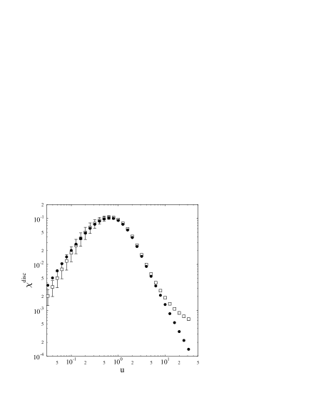
Figure 1 shows the dependence of $\chi^{\rm disc}$ on the scaled valence quark mass $u$, defined below Eq. (7), for a typical example, $L=10$ and $\beta=2.0$. Here and below, the values for $\Sigma$ are taken from Ref. [5]. (Note that the eigenvalues in [5] were measured in units of $1/(2a)$.) The results shown in Fig. 1 were obtained without spectral unfolding. We have also unfolded the lattice data, but the resulting differences in $\chi^{\rm disc}$ are negligible since the sums in Eq. (6) are dominated by small eigenvalues for which the spectral density is approximately constant. Hence, details of the unfolding procedure are irrelevant for the present investigation.

We note that the uncertainties in the Monte-Carlo data are correlated: The entire set of dots in Fig. 1 would shift up or down within the range indicated by the error bars if, e.g., the lowest eigenvalue were allowed to move within its statistical error. Our interest is focussed on the systematic deviations visible above $u\approx 7$. In order to determine these deviations, we show in Fig. 2 the ratio

$${\bf ratio}=\left(\chi^{\rm disc}_{\rm lattice}-\chi^{\rm disc}_{\rm RMT}\right)/\left(\chi^{\rm disc}_{\rm RMT}\right)\>.$$ (14)

Figure 2: The relative difference, Eq. (14), of the scaled disconnected susceptibilities for the lattice simulation (using the data from Fig. 1 with $N=10^{4}$, $\beta=2.00$, and $\Sigma=0.1247$) and chRMT.

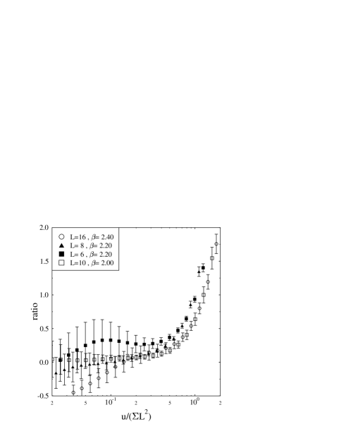
Deviations of this ratio from zero determine $\lambda_{\rm RMT}/\Delta$. The errors in Fig. 2 are jackknife estimates. Two features in the figure are striking. (i) Below the lowest eigenvalue of the Monte–Carlo sample, the errors are too small. (ii) For very small values of $u$, one observes a systematic deviation between the lattice results and the chRMT prediction. These features are artefacts of limited statistics and have the following cause. The asymptotic chRMT result for very small values of $u$ is

$$\chi^{\rm disc}\rightarrow(2u)^{2}\left[-{1\over 3}(\ln u+\gamma)-{1\over 12}\right]$$ (15)

where $\gamma$ is Euler’s constant. The logarithmic term is generated by the small but finite eigenvalue density at small $u$, see Eq. (7). However, in a given Monte–Carlo simulation there is always one smallest eigenvalue, $\lambda_{\rm min}$. For values of $u$ smaller than $\lambda_{\rm min}N\Sigma$, the logarithmic contribution can no longer be obtained from the lattice data, see Eq. (6).

Let $u_{\rm RMT}=\pi\lambda_{\rm RMT}/\Delta$ be the value of $u$ at which the strong deviation observed in Fig. 2 sets in. According to Eq. (5), $u_{\rm RMT}$ should scale with $L^{2}$ [7, 8]. To check this prediction, we have plotted in Fig. 3 the ratios defined in Eq. (14) for $L=4$, 6, 8, and 10 as a function of $u/L^{2}$. Obviously, all data fall on the same curve confirming our expectation.

Figure 3: The relative difference of the scaled disconnected susceptibilities plotted versus $u/L^{2}$ for $\beta=2.00$ and four different lattice sizes, $N=4^{4}$, $6^{4}$, $8^{4}$, and $10^{4}$.

In order to compare results for different values of $\beta$, we note that $u_{\rm RMT}$ is dimensionless but should be proportional to $L^{2}$. The latter quantity should scale with $a^{2}$, where $a$ depends on $\beta$. Furthermore, in the scaling regime one would expect that $\Sigma$ scales with $a^{-3}$. This suggests that $u_{\rm RMT}/(\Sigma^{2/3}L^{2})$ should be independent of $\beta$ in the scaling regime. Figure 4 demonstrates that this expectation is not supported by the data.

Figure 4: The relative difference of the scaled disconnected susceptibilities plotted versus $u/(\Sigma^{2/3}L^{2})$ for the data of Fig. 3 and additional data for $\beta=2.2$, $\Sigma=0.0556$ on $6^{4}$ and $8^{4}$ lattices and for $\beta=2.4$, $\Sigma=0.00863$ on a $16^{4}$ lattice.

Figure 5: The data of Fig. 4 plotted versus $u/(\Sigma L^{2})$.

It is perhaps not too surprising that simple scaling does not work, because the dynamics on the lattice changes in a highly complicated manner between $\beta=2.0$ and $\beta=2.4$. The theoretical expectation of Eq. (5) is that $u_{\rm RMT}$ should scale with $f_{\pi}^{2}L^{2}$ [7, 8]. A careful check of this expectation would require the determination of $f_{\pi}$ for the lattice sizes and $\beta$ values we have used. We have not done this. Instead, we make use of the observation [20] that $f_{\pi}^{2}$ (in lattice units) scales approximately like $\Sigma$ for the range of $\beta$ considered here. The plots in Fig. 5 showing the results for different $\beta$ versus $u/(\Sigma L^{2})$ support this view.

Billoire et al. [20] suggest that $f_{\pi}^{2}=\Sigma/3.4$ in lattice units. If one interprets Fig. 5 as indicating that $u_{\rm RMT}/(\Sigma L^{2})$ is roughly 0.5, this implies (taking into account a factor of $1/2$ from our normalization of the eigenvalues) that

$$\lambda_{\rm RMT}/\Delta\approx 0.3\,f_{\pi}^{2}L^{2}\ .$$ (16)

This result in quenched SU(2) is in agreement with the order of magnitude estimate $\lambda_{\rm RMT}/\Delta\sim f_{\pi}^{2}L^{2}/\pi$ from Refs. [7, 8].

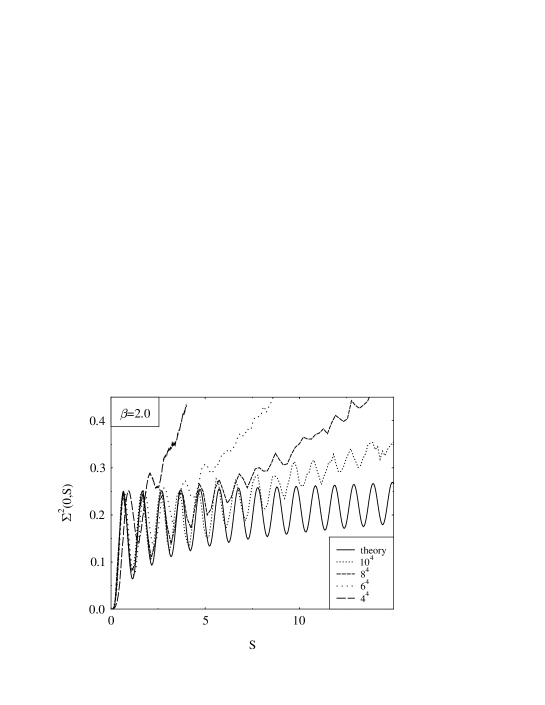
We now turn to the number variance which is defined as $\Sigma^{2}(0,S)=\langle(N(I)-\langle N(I)\rangle)^{2}\rangle$ [6]. Here, $I$ is the interval $I=[0,S]$, $N(I)$ is the number of eigenvalues in $I$, and the angular brackets denote the ensemble average. In contrast to $\chi^{\rm disc}$, unfolding is important for the $\Sigma^{2}(0,S)$ statistic since it leads to a significant extension of the length of the interval $I$ for which $\Sigma^{2}(0,S)$ can be determined. We unfolded the spectrum by fitting the unfolding function to the average of the spectrum over all configurations. Figure 6 shows that the critical value, $S_{\rm RMT}$, for which deviations from chRMT are observed increases with $L$.

Figure 6: Comparison of the number variance, $\Sigma^{2}(0,S)$, predicted by chRMT with the results for the simulations used in Fig. 3.

In Fig. 7 we see that $S_{\rm RMT}$ decreases with increasing $\beta$ as expected.

Figure 7: Same as Fig. 6 but keeping $L$ fixed and varying $\beta$.

Detailed analysis of all available data sets shows that

$$S_{\rm RMT}\approx(0.3-0.7)\,\Sigma L^{2}$$ (17)

is consistent with the data. Hence, $S_{\rm RMT}$ and $u_{\rm RMT}$ are perfectly consistent.

The use of the $\Sigma^{2}(0,S)$ statistic may be conceptually more appealing because the analogous quantity in mesoscopic systems is directly related to the Thouless energy. However, our analysis shows that the susceptibility appears to be better suited for a quantitative determination of the cross–over point from universal to non–universal behavior.

In conclusion, we have provided the first direct determination of the scale, $\lambda_{\rm RMT}$, which limits the validity of random matrix descriptions of lattice QCD. This quantity has the correct $L^{2}$-scaling. Moreover, $\lambda_{\rm RMT}$ seems to scale roughly with $f_{\pi}^{2}$ as expected on the basis of the Gell-Mann–Oakes–Renner relation.

It would be very interesting to perform a detailed analysis of the lattice data in the diffusive regime, i.e., above $\lambda_{\rm RMT}$, to check the predictions of Ref. [7] for this regime and to investigate possible differences between the numerical results of Ref. [8] for the instanton liquid model and the lattice data. Such an analysis will be the subject of future work.

It is a pleasure to thank F. Karsch and J.J.M. Verbaarschot for stimulating discussions. This work was supported in part by DFG and BMBF. SM, AS and TW thank the MPI für Kernphysik, Heidelberg, for hospitality and support. The numerical simulations were performed on a CRAY T90 at the Forschungszentrum Jülich and on a CRAY T3E at the HLRS Stuttgart.

References

- [1] For a recent review on random matrix theory in general, see T. Guhr, A. Müller-Groeling, and H.A. Weidenmüller, Phys. Rep. 299 (1998) 189.
- [2] For a review on RMT and Dirac spectra, see the recent review by J.J.M. Verbaarschot, hep-th/9710114, and references therein.
- [3] J.J.M. Verbaarschot, Phys. Lett. B 368 (1996) 137.
- [4] M.A. Halasz and J.J.M. Verbaarschot, Phys. Rev. Lett. 74 (1995) 3920.
- [5] M.E. Berbenni-Bitsch, S. Meyer, A. Schäfer, J.J.M. Verbaarschot, and T. Wettig, Phys. Rev. Lett. 80 (1998) 1146.
- [6] J.-Z. Ma, T. Guhr, and T. Wettig, Euro. Phys. J. A 2 (1998) 87.
- [7] R.A. Janik, M.A. Nowak, G. Papp, and I. Zahed, hep-ph/9803289.
- [8] J.C. Osborn and J.J.M. Verbaarschot, hep-ph/9803419.
- [9] T. Banks and A. Casher, Nucl. Phys. B 169 (1980) 103.
- [10] D. Diakonov and V. Petrov, Phys. Lett. B 147 (1984) 351; Sov. Phys. JETP 62 (1985) 204.
- [11] J. Stern, hep-ph/9801282.
- [12] T. Guhr, J.-Z. Ma, S. Meyer, and T. Wilke, hep-lat/9806003.
- [13] S. Nishigaki, Phys. Lett. B 387 (1996) 139; G. Akemann, P.H. Damgaard, U. Magnea, and S. Nishigaki, Nucl. Phys. B 487 (1997) 721.
- [14] J.J.M. Verbaarschot, Phys. Rev. Lett. 72 (1994) 2531.
- [15] K. Frahm, T. Guhr, and A. Müller-Groeling, cond-mat/9801298.
- [16] F. Karsch and E. Laermann, Phys. Rev. D 50 (1994) 6954.
- [17] E. Brézin, S. Hikami and A. Zee, Phys. Rev. E 51 (1995) 5442; A.D. Jackson and J.J.M. Verbaarschot, Phys. Rev. D 53 (1996) 7223; T. Wettig, A. Schäfer, and H.A. Weidenmüller, Phys. Lett. B 367 (1996) 28; M.A. Nowak, G. Papp, and I. Zahed, Phys. Lett. B 389 (1996) 137.
- [18] A.D. Jackson, M.K. Şener, and J.J.M. Verbaarschot, Nucl. Phys. B 479 (1996) 707, B 506 (1997) 612; T. Guhr and T. Wettig, Nucl. Phys. B 506 (1997) 589.
- [19] T. Nagao and P.J. Forrester, Nucl. Phys. B 435 (1995) 401.
- [20] A. Billoire, R. Lacaze, E. Marinari, and A. Morel, Nucl. Phys. B 251 (1985) 581.