Abstract

It is shown that the gluons produced with small transverse momenta $k_{\perp}$ inside a jet ($k_{\perp}<k_{\perp}^{cut}$, $k_{\perp}^{cut}\to 0$) are independently emitted from the primary parton, as QCD coherence suppresses their showering. Consequently, the low $k_{\perp}$ gluons follow a Poisson distribution, very much like the soft photons radiated by a charged particle in QED. On the contrary, the distribution of gluons with limited absolute momenta $|\vec{k}|<k^{cut}$ remains non-Poissonian even for small $k^{cut}$. It will be interesting to find out to what extent this perturbative prediction for partons survives the hadronization process.

1 Introduction

It is by now well established that the multiplicity distributions of hadrons produced in high energy collisions are substantially wider than the Poisson distribution. This can be understood in a large class of models based on branching processes [1], the quark gluon cascade in perturbative QCD being a relevant example [2, 3]. In this paper we point out that the specific properties of the QCD cascade allow one to select simple regions of phase space where the produced partons are less correlated and show a narrow multiplicity distribution. The experimental check of our predictions would therefore provide a novel test of the role of perturbative QCD in multiparticle production.

It is convenient to characterize the multiplicity distribution of particles in an event by its global factorial moments $f^{(q)}=<n(n-1)\ldots(n-q+1)>$ of order $q$, or, written in terms of the $q$-particle inclusive density

$$f^{(q)}(Q)=\int\rho^{(q)}(k_{1}\dots k_{q};Q)dk_{1}\dots dk_{q},$$ (1)

with an integral over the full phase space available at the energy scale $Q$ for the process. The ratios $F^{(q)}\equiv f^{(q)}/\bar{n}^{q}$ were extensively studied in perturbative QCD to various degrees of accuracy [4, 5, 6]. The asymptotic results are obtained in the Double Logarithmic Approximation (DLA) and the normalized moments approach a limit $F^{(q)}(Q)\rightarrow F_{q}$, corresponding to KNO multiplicity scaling[1, 7]. The numbers $F_{q}$ are independent of the coupling, thus providing a universal characteristic of the multiplicity distribution. These moments essentially differ from $F_{q}=1$ as for the Poisson distribution and then the asymptotic KNO distribution essentially differs from the Dirac delta function.

In analogy with (1) we define the cut moments

$$f^{(q)}_{c}(C,Q)=\int_{\Gamma_{c}(C,Q)}\rho^{(q)}(k_{1}\dots k_{q};Q)dk_{1}\dots dk_{q},$$ (2)

where the phase space integration is now restricted by $\Gamma_{c}(C,Q)$ with a cut variable $C$. In this paper we discuss two types of cuts to be applied to all particles in the final state: the momentum cut $|\vec{k}_{i}|<k^{cut}$, and the transverse momentum cut $k_{\perp,i}<k_{\perp}^{cut}$, for $i=1,...,q$. Clearly, the moments (2) determine the multiplicity distribution of particles produced in the restricted phase space, and as such they provide a more differential characteristics than the global quantities. For the maximal $k^{cut}$ and $k_{\perp}^{cut}$ at a given energy scale $Q$ the global quantities are retained.

Depending on the choice of the cut, the moments in Eq.(2) are probing quite different physical phenomena. Of special importance in this discussion is the coherence of the soft gluon emission from the harder partons which yields an angular ordering of subsequent emissions along the branching process [8]. In particular, this property leads to the suppression of the soft particle production [9] and to a flat, energy independent rapidity distribution of particles with low transverse momenta in the parton jet, reminiscent of the QED Bremsstrahlung [10].

To see the effect of the angular ordering on our cut moments consider first the momentum cut. Since the dominant source of particle production in the QCD cascade is the gluon splitting, the existence of one gluon simply enhances the probability to find another one nearby in momentum space and this yields positive correlations which do not vanish even for a small momentum cut $k^{cut}$. Such correlations would also persist with the $k_{\perp}$ cutoff if there was no angular ordering. With the angular ordering taken into account however, a cut in the transverse momentum of one parton yields an even stronger restriction of the available phase space for the next parton in the cascade, and consequently, the correlations are strongly damped near the low $k_{\perp}$ threshold. Because of this suppression of secondary emissions in the $k_{\perp}$ cut phase space one obtains ultimately the independent emission of low $k_{\perp}$ gluons and therefore a Poisson distribution very much in analogy to the multiple soft photon Bremsstrahlung in QED.

Differences between the momentum cut and $k_{\perp}$ cut moments become more pronounced towards small cutoffs. Fortunately, this is the region where the simple approximations are most reliable. We derive here the evolution equations for both types of moments, which can be solved recursively to any order of the perturbation theory within the DLA. These results provide the qualitatively correct picture as can also be inferred from the Monte Carlo simulations at the parton level.

It will be interesting to find out whether the experimental data indeed show the approach to a Poisson distribution as one might expect from the Local Parton Hadron Duality (LPHD) picture, originally proposed for single inclusive distributions [9], but successful also in a broader range of phenomena [11]. Alternatively, the hadronization process could destroy the coherence properties of the parton cascade; this happens in a specific hadronization model studied here for small $k^{cut},k^{cut}_{\perp}<1$ GeV. Hence the observation of the above regularities in the hadronic final state would provide us with a clue on the hadronization mechanism.

After presenting a few basic relations of the DLA scheme in Chapter 2, we derive in Chapter 3 the threshold behaviour of both families of cut moments in the leading perturbative order. In Chapter 4 recursive evolution equations are derived which generate perturbative expansions to arbitrary order for constant and running $\alpha_{s}$. In Chapter 5 we discuss for comparison the Monte Carlo results and conclude with Chapter 6. The Appendices contain details of various derivations and a sample of explicit expressions for cut moments up to the third non-leading correction.

2 Particle correlations in jets in DLA

In this paper we consider multiplicity distributions of hadrons or partons in a jet of primary energy $P$ and half opening angle $\Theta$ in limited regions of phase space. The multiparton correlations in a jet evolving from the primary parton $a$ ($a=q,g$) can be derived from the generating functional $Z_{P,a}$ which in DLA obeys the following integral equation [4]

$$Z_{P,a}\{u\}=\exp\left(\int_{\Gamma_{P}(K)}{\cal M}_{P,a}(K)[u(K)Z_{K,g}\{u\}-1]d^{3}K\right).$$ (3)

This equation refers to the multiparton final state excluding the leading particle. In (3) the subscript $P$ denotes collectively the momentum vector of the parent parton and the half opening angle ($P=\{\vec{P},\Theta\}$) of the jet it generates; $\Gamma_{P}(K)$ stands for the phase space of the intermediate parent $\vec{K}$, $\Gamma_{P}(K)=\{K:K<P,\Theta_{KP}<\Theta,K\Theta_{KP}>Q_{0}\}$, where $Q_{0}$ is a transverse momentum cutoff parameter). The probability ${\cal M}_{P,a}(K)$ for the bremsstrahlung of a single gluon off the primary parton $a$ reads for small angle $\Theta_{PK}$

$${\cal M}_{P,a}(K)d^{3}K=c_{a}\gamma_{0}^{2}(K\Theta_{PK})\frac{dK}{K}\frac{d\Theta_{PK}}{\Theta_{PK}}\frac{d\Phi_{PK}}{2\pi},$$ (4)

where $c_{g}=1,~{}c_{q}=C_{F}/N_{c}=4/9$ for initial gluons and quarks respectively. The multiplicity anomalous dimension is related to the strong coupling by $\gamma_{0}^{2}=2N_{C}\alpha_{s}/\pi$ and is taken as $\gamma_{0}^{2}(y)=\beta^{2}/(y+\lambda)$ where $y=\ln(k_{\perp}/\Lambda)$, $\lambda=\ln\frac{Q_{0}}{\Lambda}$ and $\beta^{2}=4N_{C}/(\frac{11}{3}N_{C}-\frac{2}{3}n_{f})$; here $N_{C}$ and $n_{f}$ denote the numbers of colours and flavours and $\Lambda$ is the QCD scale.

The inclusive densities are obtained from Taylor expansion of the generating functional around $u(k)=1$

$$\rho_{P,a}^{(q)}(k_{1},...,k_{q})=\delta^{q}Z_{P,a}\{u\}/\delta u(k_{1})...\delta u(k_{q})\mid_{u=1},$$ (5)

likewise the connected (cumulant) correlation functions from

$$\Gamma_{P,a}^{(q)}(k_{1},\ldots,k_{q})=\delta^{q}\ln Z_{P,a}\{u\}/\delta u(k_{1})\ldots\delta u(k_{q})\mid_{u=1}.$$ (6)

These differential distributions satisfy the following integral equations [14]

$$\Gamma^{(q)}_{P,a}(k_{1},\ldots,k_{q}) =d_{P,a,nest}^{(q)}(k_{1},\ldots,k_{q})+\int d^{3}K{\cal M}_{P,a}(K)\rho^{(n)}_{K,g}(k_{1},\ldots,k_{q}),$$ (7)

$$d_{P,a,nest}^{(q)}(k_{1},\ldots,k_{q}) ={\cal M}_{P,a}(k_{1})\rho_{k_{1},g}^{(q-1)}(k_{2},\ldots,k_{q})+cycl.$$ (8)

The cut moments $f^{(q)}_{c}$ are obtained as integrals over the particle density distributions $\rho^{(q)}$ as in eq. (2), likewise the cumulant moments $c^{(q)}$ as integrals over the connected correlation functions $\Gamma^{(q)}$.

The global moments integrated over full phase space can be derived more simply from the integrated generating function $Z(Y,u)$ which – in analogy to eq. (3) – fulfils the evolution equation [13]

$$Z_{a}(Y,u)=\exp\{\int^{Y}_{0}dyc_{a}\gamma^{2}_{0}(y)(Y-y)[uZ(y,u)-1]\}$$ (9)

where the evolution variable in small angle approximation is $Y=\ln\frac{P\Theta}{Q_{0}}$. The global moments are then derived from $f^{(q)}=d^{q}Z/du^{q}|_{u=1}$ and $c^{(q)}=d^{q}\ln Z/du^{q}|_{u=1}$ and we recall that these moments are related by (see, for example [12])

$$f^{(q+1)}=\sum^{q}_{m=0}{q\choose m}f^{(q-m)}c^{(m+1)}.$$ (10)

Frequently used are the moments $F^{(q)}=f^{(q)}/\bar{n}^{q}$ and $K^{(q)}=c^{(q)}/\bar{n}^{q}$ normalized by the mean multiplicity $\bar{n}\equiv f^{(1)}\equiv c^{(1)}$.

For later use we also present here the results for the global factorial moments $f^{(q-1)}$ to the lowest perturbative order, an approximation suitable for small $Y$. To this end, one obtains first, after q-fold differentiation of $\ln Z$ over $u$ in (9), the equation

$$c_{a}^{(q)}(Y)=\int^{Y}_{0}dyc_{a}\gamma^{2}_{0}(y)(Y-y)(qf^{(q-1)}(y)+f^{(q)}(y)).$$ (11)

Then, starting with $f^{(0)}$ = 1, one finds the higher moments by iteration whereby in leading order of $Y$ the second term with $f^{(q)}$ in (11) can be neglected against $qf^{(q-1)}$. After inserting (11) into (10) one obtains finally for small $Y$

$$f^{(q)}(Y)\simeq f_{q}c_{a}^{q}\gamma_{0}^{2q}Y^{2q},$$ (12)

thus the moments vanish at the threshold $Y\to 0$ ($P\Theta\to Q_{0}$). The coefficients $f_{q}$ in (12) are given recursively by

$$f_{q}=\sum^{q-1}_{k=0}\frac{f_{k}f_{q-k-1}}{2(2q-2k-1)}{q-1\choose k}$$ (13)

and the first coefficients read

$$f_{0}=1,\quad f_{1}=\frac{1}{2},\quad f_{2}=\frac{1}{3},\quad f_{3}=\frac{17}{60},\ldots.$$ (14)

Note that the relation (13) is different from the analogous relation which determines global moments at large $Y$ ([13, 14]).

3 Multiplicity Moments for small cut-off

In this section we derive the multiplicity moments for the phase space with cylindrical cut $k_{\perp}<k_{\perp}^{cut}$ and with spherical cut $k<k^{cut}$ for small parameters $k_{\perp}^{cut}$ and $k^{cut}$. In these limiting cases various simplifications can be applied: first, it is enough to take into account the terms of lowest order in the coupling. We show in the next section that terms of higher order are indeed suppressed for small transverse momenta. Secondly, in this limit, the solutions for running coupling approach those for fixed coupling, in which case close expressions can be obtained.

3.1 Cylindrical phase space

For the multiplicity in the $k_{\perp}^{cut}$ cylinder (not including the leading particle of momentum $P$) we obtain

$$\bar{n}(k_{\perp}^{cut},P,\Theta)=\int^{k_{\perp}^{cut}}_{Q_{0}}\frac{dk_{\perp}}{k_{\perp}}\gamma^{2}_{0}(k_{\perp})\int^{\Theta}_{k_{\perp}/P}\frac{d\Theta^{\prime}}{\Theta^{\prime}}=\int^{X_{\perp}}_{0}dy\gamma_{0}^{2}(y)(Y-y),$$ (15)

where $X_{\perp}=\ln\frac{k_{\perp}^{cut}}{Q_{0}}$. Now it can easily be seen that for $X_{\perp}\ll\lambda$ the variation of the coupling can be neglected and $\gamma_{0}^{2}=\beta^{2}/\lambda$. For fixed coupling we find in lowest order

$$\bar{n}(X_{\perp},Y)=\gamma^{2}_{0}X_{\perp}(Y-X_{\perp}/2),$$ (16)

which reduces for $X_{\perp}\ll Y$ to $\bar{n}(X_{\perp},Y)=\gamma^{2}_{0}X_{\perp}Y$ corresponding to a constant particle density in $\ln k_{\perp}$ and $\ln k$.

Here and in the rest of this section we write for simplicity the results for gluon jets. For quark jets the coupling $\gamma_{0}^{2}$ should be replaced by $c_{q}\gamma_{0}^{2}$ everywhere as we deal only with gluon emission from the primary parton.

The higher order moments are obtained from (7), where we neglect the second term which is of higher order in $\alpha_{s}$. The integration of $\Gamma^{(q)}$ and $\rho^{(q)}$ over the momenta yields the cumulant and factorial moments in the given region of phase space. For $k_{1}$ kept fixed the integral over $k_{2}\cdots k_{q}$ in (8) yields the global factorial moment $f^{(q)}$ at scale $k_{\perp 1}=k_{1}\vartheta_{1}$: because of angular ordering the angles in all later emissions must obey $\vartheta_{2},\cdots,\vartheta_{q}<\vartheta_{1}$. So one finds

$$c^{(q)}(X_{\perp},Y)=q\int^{X_{\perp}}_{0}dy\gamma^{2}_{0}(y)(Y-y)f^{(q-1)}(y).$$ (17)

Hence in this approximation the cut moments are determined by the global ones. Again one recovers the fixed $\alpha_{s}$ limit for small $X_{\perp}$.

For the normalized cumulant moments in the case of fixed coupling we find from (16) and (17) after inserting the moments in the approximation (12)

$$K^{(q)}(X_{\perp},Y)=\frac{2^{q-1}f_{q-1}}{2q-1}\frac{2qY-(2q-1)X_{\perp}}{(2Y-X_{\perp})^{q}}X_{\perp}^{q-1},$$ (18)

and for the case of small cut-off $k^{cut}_{\perp}$ we are interested in, i.e. for $X_{\perp}\ll Y$

$$K^{(q)}(X_{\perp},Y)=\frac{qf_{q-1}}{2q-1}\left(\frac{X_{\perp}}{Y}\right)^{q-1}.$$ (19)

Therefore, in this approximation the cumulants $K^{(q)}$ quickly decrease with the order $q$. It is interesting to note that this power like dependence on the order $q$ corresponds to the “linked pair” ansatz for correlations [15], usually written as $K^{(q)}=A_{q}[K^{(2)}]^{q-1}$, which is made in models where multi-particle correlations are built from 2-particle correlations. The higher cumulants in (19) rise more slowly than in case of the negative binomial distribution in which case $A_{q}=(q-1)!$ [16].

Finally, the factorial moments are obtained by solving (10) approximately through $F^{(q)}=1+q(q-1)K^{(2)}/2+{\cal O}(K^{(3)})$, which yields

$$F^{(q)}(X_{\perp},Y)\cong 1+\frac{q(q-1)}{6}\frac{X_{\perp}}{Y}.$$ (20)

So we obtain the remarkable result that for small transverse momentum cut-off all factorial moments approach unity and therefore the multiplicity distribution becomes Poissonian. This is a consequence of the dominance of the single soft gluon emission at small $k_{\perp}$, i.e., the absence of branching processes with secondary gluon emissions. This behaviour is just analogous to the usual QED bremsstrahlung and follows from the coherence of the soft gluon radiation and the angular ordering condition which limits the angles of the secondary particles in (17) by the (typically small) emission angle $\vartheta_{1}$ of the first gluon.

If the running of the coupling is taken into account, the computation already of the leading contributions yields quickly rather lengthy formulae with increasing order $q$. For the first two moments we find

$$\bar{n}(X_{\perp},Y)=\beta^{2}\{(Y+\lambda)\ln\frac{X_{\perp}+\lambda}{\lambda}-X_{\perp}\},$$ (21)

$$\begin{aligned} c^{(2)}(X_{\perp},Y)&=\beta^{4}\{[\lambda(4Y+3\lambda)-X_{\perp}(X_{\perp}-2Y)]\ln\frac{X_{\perp}+\lambda}{\lambda}\\ &\phantom{=\beta^{4}\{[\lambda(4Y+3\lambda)}-X_{\perp}(3\lambda+4Y-3X_{\perp}/2)\}\\ &\approx 2\beta^{4}Y\{(X_{\perp}+2\lambda)\ln\frac{X_{\perp}+\lambda}{\lambda}-2X_{\perp}\},\end{aligned}$$

where the latter approximation applies for $X_{\perp}\ll Y$. Our essential results about the behaviour of correlations for $X_{\perp}\to 0$ coincide with the results for fixed coupling as expected by the general argument.

The different approximations for the second moment $F^{(2)}$ discussed here are compared in Fig. 1. One can see that the running $\alpha_{s}$ results yield lower values for the moments with increasing $X_{\perp}$ but all results approach the same linear behaviour with the same slope for $X_{\perp}\to$ 0.

It is also interesting to note that the results (18-20) for the normalized moments are independent of the coupling $\gamma_{0}^{2}$ and therefore also independent of the colour of the primary parton, i.e. the normalized moments in quark and gluon jets approach the same limiting behaviour. The reason is that in this limit all gluons are emitted from the primary parton; this is different from the case of global moments, where only the first gluon in the cascade is emitted from the primary parton within the DLA.

3.2 Spherically cut phase space

Next we consider the multiplicity distribution in the reduced phase space with cut in the modulus of momentum $k<k^{cut}$, but still limited by the jet opening angle $\Theta$.

In the present approximations the initial momentum $P$ enters the final results only through the boundary $k<P$ if the leading particle is disregarded. This implies that we can easily construct from the previous subsection the results for the combined cuts $k_{\perp}<k_{\perp}^{cut}$ and $k<k^{cut}$ by replacing $P$ by $k^{cut}$ or $Y$ by $X=\ln(k^{cut}\Theta/Q_{0})$ in the equations for moments such as (20). We note that the largest deviations from the DLA are expected to come from the large momenta $k$ where the energy-momentum constraints and also the explicit form of the splitting functions become important. Therefore, a DLA formula like (20) becomes more realistic for restricted momenta $k<k^{cut}$, i.e., if we substitute $X$ for $Y$ keeping $X$ smaller than the global scale $Y$ at the same time.

Now the results for the spherical phase space with $k<k^{cut}$ (without additional bound on $k_{\perp}$) are obtained from the formulae of the previous subsection after letting $k_{\perp}^{cut}\to k^{cut}$ or $X_{\perp}\to X$ and also replacing $Y$ by $X$. For fixed coupling in lowest order we obtain from (18)

$$\bar{n}(X,Y) =\gamma_{0}^{2}X^{2}/2,$$ (22)

$$K^{(q)}(X,Y) =2^{q-1}f_{q-1}/(2q-1).$$ (23)

The normalized moments $K^{(q)}$ are $X$-independent. This shows the different behaviour of the cut moments in cylindrical and spherical phase space: they decrease to zero or stay constant, respectively, if the cut-off is lowered towards the kinematic limit. Consequently, as announced in the Introduction, soft gluons with limited momentum $k$ have essentially a non-Poissonian multiplicity distribution, while those with limited $k_{\perp}$ are indeed produced independently.

3.3 Role of angular ordering

In order to demonstrate the importance of angular ordering for these predictions, we arbitrarily drop this condition in the corresponding integrals. Let’s consider first the integral as in (17) in the case of the cylindrical phase space. Taking the second moment as an example, we then obtain in the approximation $X_{\perp}\ll Y$ and $\alpha_{s}$ fixed

$$c^{(2)}(X_{\perp},Y) =2\int^{\Theta}_{Q_{0}/P}\frac{d\vartheta_{1}}{\vartheta_{1}}\int^{k_{\perp}^{cut}/\vartheta_{1}}_{Q_{0}/\vartheta_{1}}\frac{dk_{1}}{k_{1}}\gamma^{2}_{0}\int^{\Theta}_{Q_{0}/k_{1}}\frac{d\vartheta_{2}}{\vartheta_{2}}\int^{k_{\perp}^{cut}/\vartheta_{2}}_{Q_{0}/\vartheta_{2}}\frac{dk_{2}}{k_{2}}\gamma^{2}_{0}$$

$$\approx\gamma_{0}^{4}X_{\perp}^{2}Y^{2}$$ (24)

where the upper limit of the $\vartheta_{2}$-integral is shifted from $\vartheta_{1}$ to $\Theta$. The result is symmetric in $X_{\perp}$ and $Y$ as is the corresponding result for the multiplicity (16) which applies also to the present discussion; then the normalized moment becomes constant

$$K^{(2)}\approx 1.$$ (25)

On the other hand, if angular ordering is taken into account, one obtains the asymmetric result (19) – corresponding to $c^{(2)}\sim X_{\perp}^{3}Y$ with the stronger $X_{\perp}$ dependence – and finally the Poisson distribution in the limit $X_{\perp}\to 0$.

Of course, angular ordering has also consequences for the results in the spherical phase space and in general reduces the correlations, for example, $K^{(2)}=\frac{1}{3}$ from (23) as compared to (25), however its consequences are less dramatic in this case. For the $k_{\perp}$ cut the primary emission angle is restricted towards small angles and then the same holds for the subsequent emission angles; in the case of spherical cut the primary emission angle is only limited by its maximum, the jet opening angle $\Theta$, and therefore the restrictions for the subsequent emissions are less severe. So the $k_{\perp}$ cut results are more sensitive to the constraints from coherence and angular ordering and therefore yield the very different results.

3.4 Alternative phase space boundaries

Finally in this section, we want to discuss a different upper bound for the momenta which connects to other results. In case of cylindrical cut we have considered so far the trapezoidal boundaries $Q_{0}\leq k_{\perp}\leq k_{\perp}^{cut}$ and $k_{\perp}/\Theta<k<P$. In this case $X_{\perp}\leq Y$ where $X_{\perp}=Y$ corresponds to the triangular boundary of the spherical cut. For comparison we consider now a phase space boundary which is given by a second cone with opening angle $\Theta^{\prime}<\Theta$. In this case the upper limit of $k$, at fixed $k_{\perp}$, becomes $k<k_{\perp}/\Theta^{\prime}$. Then the angular integrals factorize and, instead of (16) and (18) one finds simply

$$\bar{n}(X_{\perp},\Delta Y) =\gamma_{0}^{2}X_{\perp}\Delta Y$$ (26)

$$K^{(q)} =\frac{qf_{q-1}}{2q-1}\left(\frac{X_{\perp}}{\Delta Y}\right)^{q-1}$$ (27)

where $\Delta Y=\ln(\Theta/\Theta^{\prime})$ denotes the rapidity difference of the angular boundaries. These results again clearly demonstrate the different roles of longitudinal and transverse directions: for $X_{\perp}\ll\Delta Y$ the correlations vanish because of angular ordering as discussed above and the formulae (26) and (27) correspond to the results (16) and (19) for small $X_{\perp}$ with $Y$ replaced by $\Delta Y$; on the other hand, for $X_{\perp}\gg\Delta Y$ the collection of the many produced partons yields large correlations. In fact, in this configuration the higher orders become important with increasing $X_{\perp}$ and the fractal structure of the parton cascade yields the power behaviour of the correlations (“Intermittency”) [14, 17, 18]. Eq. (27) nicely demonstrates the different trends $K^{(q)}\to 0$ and $K^{(q)}\to\infty$ for $X_{\perp}\to 0$ and $\Delta Y\to 0$ respectively.

4 Multiplicity moments in higher orders

In this section we derive the integral evolution equations for factorial moments in the cut phase space. These equations will then be used to generate in the systematic way higher order corrections to the required accuracy. The complete solution obtained in this way gives cut moments for the full range of the cut-offs $0<X,X_{\perp}<Y$. It reduces to the Born approximation at the threshold, thus justifying simplifications used in the previous Section. For simplicity, only the gluon jets will be considered in this section, hence we set $c_{a}=1$.

All evolution equations, which we seek for, follow from Eqs.(7,8) together with (10) which is also valid in the restricted phase space. To begin we first simplify Eqs.(7) employing the pole approximation [14]. This essential step consists of saturating the angular integration in (7) over the intermediate parent momentum $\vec{K}$ by the leading singularities of the integrand. This amounts to approximating $\vec{K}\parallel\vec{k_{i}}$ in all nonsingular terms and integrating only over the smallest angle $\Theta_{Kk_{i}}$, $k_{i}=1\dots n$. This leads to the following equation for the single parton density differential in momentum $k$ and angle $\vartheta$ [14]

$$\rho^{(1)}(\vartheta,k,P)={{\gamma_{0}^{2}}(k\vartheta)\over k\vartheta}+\frac{1}{\vartheta}\int_{k}^{P}{dK\over K}\int_{Q_{0}\over k}^{\vartheta}{d\Theta_{Kk}\over\Theta_{Kk}}\gamma_{0}^{2}(K\vartheta)\left[\Theta_{Kk}\rho^{(1)}(\Theta_{Kk},k,K)\right],$$ (28)

For the fully differential two-parton connected correlation function

$$\Gamma_{P}^{(2)}(\vartheta_{1},\vartheta_{2},k_{1},k_{2})=\Gamma_{1}^{(2)}(\vartheta_{1},\vartheta_{12},k_{1},k_{2},P)+\Gamma_{2}^{(2)}(\vartheta_{2},\vartheta_{12},k_{2},k_{1},P),$$ (29)

we obtain

$$\Gamma^{(2)}_{1}(\vartheta_{1},\vartheta_{12},k_{1},k_{2},P)={\cal M}_{P}(k_{1})\rho^{(1)}(k_{2},\vartheta_{2},K)+\frac{1}{\vartheta_{1}}\int_{k_{>}}^{P}\frac{dK}{K}\gamma_{0}^{2}(K\vartheta_{1})$$ (30)

$$\left\{\int_{Q_{0}/k_{1}}^{\vartheta_{12}}d\Theta_{Kk_{1}}\rho^{(1)}(\Theta_{Kk_{1}},k_{1},K)\rho^{(1)}(\vartheta_{12},k_{2},K)+\right.$$

$$\left.\int_{\vartheta_{12}}^{\vartheta_{1}}d\Theta_{Kk_{1}}\Gamma^{(2)}_{1}(\Theta_{Kk_{1}},\vartheta_{12},k_{1},k_{2},K)\right\}.$$

with the polar angle $\vartheta_{i}$ of particle $i$, the relative polar angle $\vartheta_{12}$ of two particles and $k_{>}=\max\{k_{1},k_{2}\}$. Note the different bounds on $\Theta_{Kk_{1}}$ in the two terms. They follow from the different singularity structure of the product term and of the connected correlation function. The splitting (29) is a consequence of the pole approximation – $\Gamma^{(2)}_{i}$ results from the saturation of the $d^{3}K$ integration in Eq.(7) by the $\vec{K}\parallel\vec{k}_{i}$ configuration.

Analogous simplifications of the evolution equations can be made for higher order densities.

4.1 Evolution equations for momentum cut moments

Integrating Eq.(28) over the spherically cut phase space of the single parton in a jet $(P,\Theta)$ gives for the average multiplicity

$$\bar{n}(k^{cut},P\Theta)=\bar{n}(k^{cut}\Theta)+\int_{Q_{0}/k^{cut}}^{\Theta}{d\vartheta\over\vartheta}\int_{k^{cut}}^{P}{dK\over K}{\gamma_{0}^{2}}(K\vartheta)\bar{n}(k^{cut},K\vartheta),$$ (31)

The structure of this equation can be simply understood from the general rules of the angular ordering and transverse momentum limitations. Since the momentum of a child parton is limited by $k^{cut}$, their emission angles are bounded from below by $Q_{0}/k^{cut}$. Because of the angular ordering, this also limits from below the emission angle $\vartheta$ of the intermediate parent $K$. The remaining phase space of $(K,\vartheta)$ can be conveniently split into $K<k^{cut}$ and $K>k^{cut}$, c.f. regions (I) and (II) in Fig. 2. Parents in the first region contribute to the global multiplicity at the scale $k^{cut}$ and parents from the second region give rise to the second term of Eq. (31). In Appendix A we derive an analogous equation for the second cumulant, by following the above steps in detail.

Similarly, one derives the evolution equations for higher moments. We obtain for the cumulants $c^{(q)}(k^{cut},P\Theta)=c^{(q)}(X,Y)$ in the logarithmic variables $X=\ln{(k^{cut}\Theta/Q_{0})}$ and $Y=\ln{(P\Theta/Q_{0})}$

$$c^{(q)}(X,Y)=\int_{0}^{X}dy{\gamma_{0}^{2}}(y)[qf^{(q-1)}(y)+f^{(q)}(y)](X-y)$$ (32)

$$+\int_{0}^{X}dx\int_{x}^{Y-X+x}dy{\gamma_{0}^{2}}(y)f^{(q)}(x,y).$$

This, together with Eqs.(10,11) , uniquely determines all multiplicity moments in the spherically cut phase space. The lowest order contributions are given recursively, in $q$, by the first integral with the $f^{(q-1)}$ term only. Perturbative expansion in the order $O({\gamma_{0}^{2}}^{k})$ can now be generated recursively in $q$ and $k$ by integrating the $O({\gamma_{0}^{2}}^{k-1})$ expansion according to Eq.(32). For constant $\alpha_{s}$ this was done for the first four moments up to terms $O({\gamma_{0}^{2}}^{8})$ with the results shown in Fig. 3. A sample of explicit expressions is given in the Appendix B.

In the global limit $(X\rightarrow Y)$ the second integral disappears, and the above equations reduce to the known equations (11) for the global moments.

Since the lowest order is also given by the first integral, the Born approximation for the normalized moments is independent of the maximum virtuality $P\Theta$ and equals to the global moments at the scale $k^{cut}\Theta$. Consequently, the normalized moments are constant in this approximation and are determined by the coefficients (13). In the higher orders they aquire a mild $X$ dependence due to the additional radiation from parents which are faster than the cut-off $k^{cut}$.

As already mentioned, while the higher order corrections are of course important for the unnormalized moments, they largely cancel in the ratios $F^{(q)}$. As a consequence, the Born approximation discussed in the previous chapter reproduces rather reliably the properties of these moments, especially the difference between the spherically and cylindrically cut moments.

This scheme applies for the running $\alpha_{s}$ case as well, and higher order corrections can be generated by the same, albeit more tedious steps.

4.2 Cylindrically cut moments

4.2.1 Multiplicity for constant $\alpha_{s}$

Integrating Eq.(28) over the parton momentum $k$ at fixed $k_{\perp}$ gives the evolution equation for the inclusive $k_{\perp}$ distribution

$$\rho(k_{\perp},P\Theta)=b(k_{\perp},P\Theta)+{{\gamma_{0}^{2}}\over k_{\perp}}\int_{k_{\perp}/\Theta}^{P}{dK\over K}\int_{Q_{0}}^{k_{\perp}}d\kappa_{\perp}\rho(\kappa_{\perp},K\Theta{\kappa_{\perp}\over k_{\perp}})$$ (33)

with the Born term $b={\gamma_{0}^{2}}\ln{(P\Theta/k_{\perp})}/k_{\perp}$. Note that the kinematics of this equation is very different from that for the absolute momentum distribution. While in the latter the rotationally invariant momentum of a child parton is the same for the P-jet and for the internal K-jet, in the former the transverse momenta $k_{\perp}$ and $\kappa_{\perp}$ refer to different axes, see Fig. 4. This leads to the more complicated structure of Eq.(33). In particular, the virtuality of the internal K-jet depends now on $\kappa_{\perp}$. In fact the effective angle $\bar{\vartheta}=\Theta\frac{\kappa_{\perp}}{k_{\perp}}$ should be interpreted as the angle between the momentum of the parent $\vec{K}$ and the parton emitted at the maximal angle $\Theta$ which is allowed. In this variable, Eq.(33) has a simple interpretation.

Integrating Eq.(33) over $k_{\perp}$ up to the transverse cut-off $k_{\perp}^{cut}$, we obtain for the average multiplicity of partons with limited $k_{\perp}$

$$\bar{n}(k_{\perp}^{cut},P\Theta)=\bar{n}_{b}(k_{\perp}^{cut},P\Theta)+$$ (34)

$${\gamma_{0}^{2}}\int_{Q_{0}/\Theta}^{k_{\perp}^{cut}/\Theta}{dK\over K}\int_{Q_{0}/K}^{\Theta}{d\bar{\vartheta}\over\bar{\vartheta}}\bar{n}(K\bar{\vartheta})+$$

$${\gamma_{0}^{2}}\int_{k_{\perp}^{cut}/\Theta}^{P}{dK\over K}\int_{Q_{0}\Theta/k_{\perp}^{cut}}^{\Theta}{d\bar{\vartheta}\over\bar{\vartheta}}\bar{n}(k_{\perp}^{cut}{\bar{\vartheta}\over\Theta},K\bar{\vartheta}).$$

where $\bar{n}_{b}$ denotes the Born contribution, Eq.(16). Similarly to the spherical case, the phase space of the intermediate parent is divided into two regions. In the first integral the maximum virtuality of the K-jet is limited by $k_{\perp}^{cut}$, therefore all partons in that jet are below cut-off, hence the global multiplicity contributes. In the second integral some partons may exceed the external cut-off $k_{\perp}^{cut}$, thus only cut multiplicity contributes. The cut $\kappa_{\perp}^{max}=(k_{\perp}^{cut}/\Theta)\bar{\vartheta}$ corresponds to the hardest parton compatible with the cut-off $k_{\perp}^{cut}$ emitted from the parent K at angle $\bar{\vartheta}$. The above equation reproduces the exact solution which can also be obtained, in the case of constant $\alpha_{s}$, by direct integration of the known fully differential distribution.

4.2.2 Relation between spherically and cylindrically cut moments

We have seen that the natural variable appearing in the $k_{\perp}$ cut case is the angle between the hardest parton in an original $(P,\Theta)$ jet and the intermediate parent $K$. One can however reorganize the calculation such that the phase space of the intermediate parton K is parametrized by its momentum and the angle $\Theta_{PK}$ at which it was emitted from the original parent $P$. This formulation provides very useful relations between both families of cut moments, valid also for running $\alpha_{s}$. It will be used to generate cylindrically cut moments to higher orders.

We begin again with the first moment, i.e. the average multiplicity written as, c.f. Fig. 5

$$\bar{n}(k_{\perp}^{cut},P\Theta)=\bar{n}(k_{\perp}^{cut})+\int_{k_{\perp}^{cut}/P}^{\Theta}d\vartheta\int_{Q_{0}/\vartheta}^{k_{\perp}^{cut}/\vartheta}dk\rho^{(1)}(\vartheta,k,P).$$ (35)

Due to the independence of the fully differential distribution on the opening angle $\Theta$, the integration over the small angles of the emitted partons $Q_{0}/P<\vartheta<k_{\perp}^{cut}/P$ results in the global multiplicity at the scale $k_{\perp}^{cut}$ (region A in Fig. 5). The second term represents contribution from the region B. We use now the Eq.(28) to express the last term by the contributions from the intermediate parents. Rearranging the integrals gives after some algebra

$$\bar{n}_{cyl}(X_{\perp},Y)=\bar{n}(X_{\perp})+(Y-X_{\perp})\int_{0}^{X_{\perp}}{\gamma_{0}^{2}}(y)[1+\bar{n}(y)]dy$$ (36)

$$+\int_{X_{\perp}}^{Y}(Y-y){\gamma_{0}^{2}}(y)\bar{n}_{sph}(X_{\perp},y)dy.$$

where the subscripts distinguish different cuts, and logarithmic variables are used. Here and in the following the quantities without subscripts and one argument refer to the global quantities. This equation allows to calculate $k_{\perp}$-cut multiplicity if the momentum cut result is known. Using the constant $\alpha_{s}$ solution of Eq.(31) we have reproduced with the aid of (36) perturbative expansion of $\bar{n}_{cyl}$ to $O({\gamma_{0}^{2}}^{12})$.

This approach generalizes for the moments of arbitrary order. We begin with the $q=2$ case and display explicitly the relevant two-parton phase space for the global cumulant

$$c^{(2)}(P\Theta)=2\int_{Q_{0}/P}^{\Theta}d\vartheta_{1}\int_{Q_{0}/P}^{\vartheta_{1}}d\vartheta_{12}\int_{Q_{0}/\vartheta_{12}}^{P}dk_{1}\int_{Q_{0}/\vartheta_{12}}^{P}dk_{2}\Gamma^{(2)}_{1}(\vartheta_{1},\vartheta_{12},k_{1},k_{2},P),$$ (37)

where $\Gamma^{(2)}_{1}$ defined as in Eq.(29). The factor $2$ comes from the symmetric $(1\leftrightarrow 2)$ configuration. Fully differential connected correlation functions in the leading logarithmic accuracy depend only on one angle relative to the original parent momentum, e.g. $\vartheta_{1}$. Direction of the second particle enters only via the relative angle $\vartheta_{12}$. Moreover for $\vartheta_{12}>\vartheta_{1}$ the connected correlation function vanishes - yet another manifestation of the angular ordering [14]. Finally, the fully differential connected correlation function is independent of the global opening of the original jet as in the single parton case. The last property allows us to split the cut cumulant into two parts as previously

$$c_{cyl}^{(2)}(k_{\perp}^{cut},P\Theta)=c^{(2)}(k_{\perp}^{cut})+2\int_{k_{\perp}^{cut}/P}^{\Theta}d\vartheta_{1}\int_{\vartheta_{1}Q_{0}/k_{\perp}^{cut}}^{\vartheta_{1}}d\vartheta_{12}$$ (38)

$$\int_{Q_{0}/\vartheta_{12}}^{k_{\perp}^{cut}/\vartheta_{1}}dk_{1}\int_{Q_{0}/\vartheta_{12}}^{k_{\perp}^{cut}/\vartheta_{1}}dk_{2}\Gamma^{(2)}_{1}(\vartheta_{1},\vartheta_{12},k_{1},k_{2},P).$$

Since the leading singularities are generated from the region where in fact $\vartheta_{12}\ll\vartheta_{1}$, the measured transverse momentum of the second parton $k_{2\perp}\sim k_{2}\vartheta_{1}$ and this gives the upper limit of the $k_{2}$ integration in (38). Inserting now Eq.(30) under the integral in (38) and rearranging various integrals gives the final expression for the cylindrically cut cumulants in terms of the global and the spherically cut factorial moments. Details of this calculations are presented in Appendix C.

Similar steps allow to derive analogous relations for cumulants of arbitrary order $q$. We obtain

$$c^{(q)}_{cyl}(X_{\perp},Y)=c^{(q)}(X_{\perp})+$$ (39)

$$(Y-X_{\perp})\int_{0}^{X_{\perp}}{\gamma_{0}^{2}}(y)[qf^{(q-1)}(y)+f^{(q)}(y)]dy+$$

$$\int_{X_{\perp}}^{Y}(Y-y){\gamma_{0}^{2}}(y)f^{(q)}_{sph}(X_{\perp},y)dy.$$

In fact Eq.(36) is the special case of this relation for $q=1$ since $f^{(0)}=1$.

Together with Eqs.(32) this equation uniquely determines all moments with limited $k_{\perp}$. We have used these equations to generate algebraically the perturbative expansion of the first four moments up to the eight order in ${\gamma_{0}^{2}}$ for constant $\alpha_{s}$, see Fig.3 and Table 4. We quote only the first nontrivial example - the $O(\alpha_{s}^{3})$ correction for $c^{(2)}$

$$c^{(2)}_{cyl,3}(X_{\perp},Y)={7\over 72}X_{\perp}^{6}-{1\over 4}X_{\perp}^{5}Y+{1\over 6}X_{\perp}^{4}Y^{2}.$$ (40)

This result was confirmed independently by the direct integration of the resolvent representation for $\rho^{(2)}$ [14] and also from the first explicit iteration of Eq.(7).

4.3 Properties of the higher order results

Fig. 3 shows spherically and cylindrically cut moments up to $O(\alpha_{s}^{8})$ in the full range of the cut-off. First three normalized moments are displayed. All properties discussed earlier are fully confirmed by this calcuation. For small cutoffs all cylindrically cut moments tend to unity while those with limited momentum have different limits corresponding to the non-Poissonian multiplicity distribution of soft gluons. The perturbative expansion is rather poorly convergent for the unnormalized moments which, being polynomials in the cut-off and $Y$, grow faster for higher order $k$. However this growth is largely canceled in the ratios. As a consequence, perturbative expansion is remarkably stable for the normalized moments $F^{(q)}$. This is clearly seen in Fig. 3 where different lines, corresponding to different maximum order $k_{max}$ included, group together for each $q$ and each type of the cut-off. In the global limit $X_{\perp},X=Y$ spherically and cylindrically cut moments are equal. However this common value, which is in fact given by the global moment, does vary with the order of the perturbative approximation. This is seen in Fig. 3 as well. This dependence is very weak and corresponds, for large $Y$, to the difference between the coefficients which determine the threshold behaviour (see Eq.(13)) and the asymptotic behaviour (see [14]), respectively, of the global moments.

5 Monte Carlo results

We have studied the behaviour of the cut moments within a Monte Carlo program in order to check our analytical calculations with a more complete numerical method, which is important in the test of the LPHD picture. In view of the similarity of its scheme with our analytical framework, we have chosen the ARIADNE program[19], in which the perturbative phase is terminated by a cutoff in transverse momentum and, in its default version, followed by string fragmentation. In deviation from the default value, the cutoff $Q_{0}$ for partons can be chosen close to the QCD scale $\Lambda$ as required in the LPHD picture, which is not easily possible in other popular QCD Monte Carlo models.

For our applications we have then switched off the hadronization phase within ARIADNE and directly compared the result at the end of the perturbative evolution with our theoretical predictions. We have reset the values of the parameters $Q_{0}$ and $\Lambda$ in ARIADNE in order to directly reproduce the energy dependence of the average multiplicity of all (charged plus neutral) hadrons according to the LPHD picture. We estimated the full (charged plus neutral) multiplicity as 3/2 the measured multiplicity for charged hadrons and we fixed the overall normalization factor which relates partons to all hadrons to $K_{all}$ = 1, as suggested by previous studies on the average multiplicity[20]. Table 1 shows a sample of parton multiplicities obtained by ARIADNE for different parameters $Q_{0}$ and $\Lambda$. By comparing the parton results with the experimental data on all hadrons, one concludes that the best set of parameters is given by $Q_{0}$ = 0.2 GeV and $\lambda$ = 0.015. It is remarkable to notice that the same value of $\lambda$ has been obtained in previous studies on jet and particle multiplicities[20], whereas the present value of $Q_{0}$ is slightly smaller than in the previous case. This difference can be related to the different approximation schemes applied.

		$\sqrt{s}$ = 91.2 GeV	$\sqrt{s}$ = 14 GeV
		$\bar{n}_{all}=31.0\pm 1.1$	$\bar{n}_{all}=13.95\pm 0.65$
$Q_{0}$	$\lambda$	$\bar{n}_{p}$	$\bar{n}_{p}$
0.6 (def.)	1 (def.)	8.21	4.2
0.27	0.1	19.2	9.7
0.27	0.01	24.8	12.5
0.23	0.01	29.4	13.4
0.2	0.015	30.2	13.8

Table 1: Predictions by ARIADNE at parton level for the total average multiplicity $\bar{n}_{p}$ in $e^{+}e^{-}$ annihilation at $\sqrt{s}$ = 14 and 91.2 GeV for different values of the parameters $Q_{0}$ and $\lambda$, compared with the experimental results for all hadrons $\bar{n}_{all}$ (taken as 3/2 the value for charged hadrons).

As a further test of LPHD, let us compare the predictions of ARIADNE using the new parameters with experimental data on factorial moments in one hemisphere as measured by the OPAL Collaboration[21]. This is done in Table 2, which clearly gives further evidence in support of LPHD using the Monte Carlo results at the parton level. In this comparison we have assumed that the normalized higher order global moments, $F_{q}$, are equal for charged hadrons and for all hadrons.

After having fixed the set of parameters of ARIADNE which are consistent with the picture of LPHD, let us now study the predictions for the cut moments at parton level; the dependence of the $k_{\perp}^{cut}$ and $k^{cut}$ moments on the cut parameter in one hemisphere defined via the thrust axis is shown in Fig. 6. According to our analytical calculations, we expect that the $k_{\perp}$ moments approach unity as $\ln k_{\perp}/Q_{0}$ for $k_{\perp}\to Q_{0}$. The cut moments predicted by ARIADNE show indeed such behaviour for small values of the cut, $k_{\perp}^{cut}\leq$ 4 GeV; however, at very small $k_{\perp}^{cut}\to Q_{0}$, the moments do not reach the predicted Poissonian value of 1, but saturate at a value larger than 1. Such effects are expected from threshold effects close to the infrared cutoff, in particular, from the boost needed to relate the overall rest frame of the collision to the single dipole rest frame where each new emission takes place.

The $k^{cut}$ moments in Fig. 6b rise to rather large values at intermediate scales and bend at small $k^{cut}$; the important point here is that they reach finite values much above unity, showing that in spherically symmetric phase space there is no Poissonian regime at very small momentum cuts. Both types of moments approach the same values for large $k_{\perp}^{cut}\sim k^{cut}$ corresponding to the global moments as it should be.

To investigate in more detail the behaviour of the $k_{\perp}$ moments in the kinematic region close to $Q_{0}$, let us now examine a new simulation with the same value of $\lambda$ but the larger value $Q_{0}$ = 0.4 GeV. Results of this run are shown in Fig. 7 for both $k_{\perp}^{cut}$ and $k^{cut}$ moments. In this case, in which the cascade is stopped earlier, the situation is clearer: the $k_{\perp}$ moments approach the Poissonian value one for $k_{\perp}^{cut}\to Q_{0}$ as theoretically expected, and stay there below the cutoff. The $k^{cut}$ moments saturate, on the other hand, at values above one as before.

	$\bar{n}$	$F^{(2)}$	$F^{(3)}$	$F^{(4)}$
Partons	30.18	1.09	1.30	1.68
Hadrons	$30.3\pm 0.6$	$1.0820\pm 0.0052$	$1.275\pm 0.019$	$1.637\pm 0.047$

Table 2: The mean multiplicity $\bar{n}$ ($\bar{n}_{p}$ or $\bar{n}_{all}$) and the first three normalized factorial moments in one hemisphere defined through the thrust axis predicted by ARIADNE at parton level with parameters $Q_{0}$ = 0.2 GeV and $\lambda$ = 0.015 and experimentally measured by the OPAL Collaboration[21]. Errors on data are the sum of statistical and systematic errors.

From these results we conclude that the more complete Monte Carlo calculation confirms the essential features of our analytical calculation in the region of small cut variables: for the $k_{\perp}^{cut}$-cut the moments vanish linearly as $\ln(k_{\perp}^{cut}/Q_{0})$, whereas for the $k^{cut}$-cut the moments approach a constant value. However, the slope and the constant values are different from the analytical predictions and also the dependence for large values of the cut momentum. We attribute these differences to our simplified DLA calculations which does not take into account energy conservation constraints and the nonleading parts of the parton splitting functions.

Finally, we show in Fig. 8 the predictions for the cut moments both with cylindrical and spherical cuts obtained at hadron level by running ARIADNE with default parameters for $e^{+}e^{-}$ annihilations at $cms$ energy of LEP-1. Data refer again to particles in one hemisphere, defined through the thrust-axis. Electrons and positrons have been subtracted to avoid the lepton contaminations of the hadronic signal; by keeping the electron pairs, a peak at very low values of the cut momentum would appear, masking the eventual physical signal. This result is consistent with an old observation[22] done within the study of intermittency phenomena that $e^{+}e^{-}$ pairs from $\pi^{0}$ decays strongly affect the experimental results in very short-range correlations.

As expected, for large values of the cut, the two moments go to a common value corresponding to the global moments of the multiplicity distribution without any cut; the obtained results are close but up to about 10% smaller than the experimental values for the global moments directly measured by the OPAL Collaboration[21]. For small values of the cut, the two moments show a different behavior; the cylindrical symmetric cut moments for $k_{\perp}^{cut}\leq 5$ GeV first tend towards unity, in agreement with our theoretical expectations; however, they rise again for very small values of the cut. This effect does not occur at the parton level and therefore has to be associated with hadronization corrections, in particular production and decay of resonances. The spherical symmetric cut moments show a step around a few GeV’s which separates two plateaus. The depletion at large $k^{cut}$ could be interpreted again as the result of energy-momentum constraints not included in our DLA calculations. It is remarkable to notice that the moments saturate and do not fall down for small values of the cut momentum, very much like in our analytical calculation. However, in view of the parton level results for the same quantity we consider this coincidence as accidental.

By comparing the partonic and the hadronic predictions, one sees that the LPHD is approximately confirmed within ARIADNE at the level of global moments and for large values of the cut momenta (right hand side of the plots) but is clearly violated for soft particles (left hand side of the plots). So we conclude that the parton level predictions show indeed the peculiar features predicted analytically within the perturbative approach, namely the near Poissonian production of soft particles as consequence of coherent multigluon emission, whereas the same features are softened and partly washed out in the model with string fragmentation. It will be interesting to find out the experimental situation.

6 Conclusions

We suggest analysing multiparticle production in restricted phase space regions with variable cut $k^{cut}_{\perp}$ in the transverse momenta of the particles, and, for comparison, with variable momentum cut $k^{cut}$. We have derived the evolution equations for the multiplicity moments within the DLA of perturbative QCD, from which their dependence on the jet virtuality and on both cut variables can be obtained. Results for moments up to order $q=4$ are given explicitly in case of fixed coupling by the first terms of the perturbative expansion.

The normalized factorial moments are found to approach a linear behaviour for small values of the transverse momentum cut with $F^{(q)}\to 1$ for $k^{cut}_{\perp}\to Q_{0}$ corresponding to a Poisson distribution, as the parton showering is uniformly suppressed at small $k_{\perp}$ for any rapidity. On the other hand, for the momentum cut, this is not the case and the moments approach a finite value for the minimal value of $k^{cut}$.

The DLA takes into account only the leading singularities but respects the soft gluon coherence which is implemented through the angular ordering prescription. We have shown that this property is responsible for obtaining a Poisson distribution in the soft limit. As a check of our analytical results, we have compared them with the results of a parton Monte Carlo program which fully takes into account the constraints from energy-momentum conservation and the complete parton splitting functions. The factorial moments for decreasing $k^{cut}_{\perp}$ continuously decrease to values close to unity, contrary to the case of the momentum cut, as expected from the analytical calculations. At the quantitative level, however, the DLA results show considerable deviations from those of the more realistic Monte Carlo calculations, as already observed in the case of global moments.

It will be interesting to find out to what extent the experimental data follow the perturbative results as one might expect from previous successes of the LPHD picture. Final state interactions, in particular resonance production, could severely disturb the perturbative results, especially in the soft region, as it is suggested indeed by the results of a Monte Carlo program which implements a model of the hadronization phase. By the proposed studies the limitations of the perturbative predictions could be explored in genuine multiparticle correlations.

Appendix A

We derive here the evolution equation for the second cumulant in the spherically cut phase space following in detail the steps outlined in Section 4.1 . Integrating Eqs.(7,8) for $q=2$ gives

$$c^{(2)}(k^{cut},P,\Theta)=2\int_{k_{1}<k^{cut}}d^{3}k_{1}{\cal M}_{P}(k_{1})\int_{k_{2}<k^{cut}}d^{3}k_{2}\rho^{(1)}_{k_{1}}(k_{2})$$ (41)

$$+\int_{\Gamma_{I+II+III}}d^{3}K{\cal M}_{P}(K)\int_{k_{1}<k^{cut}}d^{3}k_{1}\int_{k_{2}<k^{cut}}d^{3}k_{2}\rho^{(2)}_{K}(k_{1},k_{2}),$$

where the order of integrals in the second term was interchanged. The full phase space of the intermediate parent $\vec{K}$ is displayed in Fig.2. As in the one-parton case, only regions I and II contribute since both momenta of final partons are limited from above by the cut-off $k^{cut}$. This in turn restricts from below their emission angles and consequently, due to the angular ordering, the emission angle of the parent $K$. We then split explicitly the remaining integral into regions $\Gamma_{I}$ and $\Gamma_{II}$. Simplifying also the first term gives

$$c^{(2)}(k^{cut},P,\Theta)=2\int_{Q_{0}/k^{cut}}{d\vartheta_{1}\over\vartheta_{1}}\int_{Q_{0}/\vartheta_{1}}{dk_{1}\over k_{1}}{\gamma_{0}^{2}}(k_{1}\vartheta_{1})\bar{n}(k_{1}\vartheta_{1})$$ (42)

$$+\int_{Q_{0}/k^{cut}}^{\Theta}{d\vartheta\over\vartheta}\int_{Q_{0}/\vartheta}^{k^{cut}}{dK\over K}{\gamma_{0}^{2}}(K\vartheta)f^{(2)}(K\vartheta)$$

$$+\int_{Q_{0}/k^{cut}}^{\Theta}{d\vartheta\over\vartheta}\int_{k^{cut}}^{P}{dK\over K}{\gamma_{0}^{2}}(K\vartheta)f^{(2)}_{c}(k^{cut},K,\vartheta).$$

In the first term, the $k_{2}$ integral gave just the global average multiplicity at the scale $k_{1}\vartheta$ since the restriction $k_{2}<k^{cut}$ is weaker than $k_{2}<k_{1}<k^{cut}$ which is satisfied for this subprocess anyway. Similarly in the second term, momentum of the parent $K$ in the region $\Gamma_{I}$ is smaller than the cut-off, hence the phase space of the final partons is not restrited by $k^{cut}$ but by the momentum of the parent $K<k^{cut}$. Therefore the global moment at the scale $K\vartheta$ results. On the other hand in the third term a parent $K$ is harder than the cut-off and phase space of the final partons is indeed restricted by $k^{cut}$. Consequently integrating over $k_{1}$ and $k_{2}$ gives the cut moment. It is natural to introduce the logarithmic variables $Y=\ln(P\Theta/Q_{0})\;X=\ln(k^{cut}\Theta/Q_{0})$. Then $c^{(2)}(k^{cut},P,\Theta)=c^{(2)}(X,Y)$. Finally we observe that, due to the evolution equation for the global moments, Eq.(11), the first two terms combine into the global cumlant at the scale $k^{cut}\Theta$, hence

$$c^{(2)}(X,Y)=c^{(2)}(X)+\int_{0}^{X}dx\int_{x}^{Y-X+x}dy{\gamma_{0}^{2}}(y)f^{(2)}(x,y).$$ (43)

Appendix B

In this Appendix we collect a sample of higher order expressions for the cut moments. The perturbative expansion for a generic (spherically or cylindrically cut) moment reads

$$f_{k_{max}}^{(q)}(Z,Y)=\sum_{k=q}^{k_{max}}{\gamma_{0}^{2}}^{k}f^{(q)}_{k}(Z,Y),$$ (44)

where the cut-off $Z=X$ for moments in a spherical phase space and $Z=X_{\perp}$ for a cylindrical cut. Our results for the coefficients $f^{(q)}_{sph,k}(X,Y)$ and $f^{(q)}_{cyl,k}(X_{\perp},Y)$ are shown in Table 3 and Table 4 respectively. The formulas for the spherically cut moments were generated (by Mathematica) recursively in $k$ and in $q$ from the evolution equation, Eq.(32) coupled with Eq.(10). The formulas for cylindrically cut moments were obtained by integrating spherically cut moments according to Eq.(39). As one of the consistency tests we have checked that the results obtained from Tables 3 and 4 for the normalized moments $F_{k_{max}}^{(q)}=f_{k_{max}}^{(q)}/(f_{k_{max}}^{(1)})^{q}$, in the leading order of $X$ and $X_{\perp}/Y$, agree with those from Eqs. (23) and (20) respectively.

q	k	$f^{(q)}_{sph,k}(X,Y)$
	1	$\frac{{X^{2}}}{2}$
1	2	$-\frac{{X^{4}}}{8}+\frac{{X^{3}}Y}{6}$
	3	$\frac{{X^{6}}}{72}-\frac{{X^{5}}Y}{30}+\frac{{X^{4}}{Y^{2}}}{48}$
	2	$\frac{{X^{4}}}{3}$
2	3	$\frac{{X^{6}}}{18}+\frac{7{X^{5}}Y}{30}$
	4	$\frac{{X^{8}}}{240}+\frac{19{X^{7}}Y}{630}+\frac{49{X^{6}}{Y^{2}}}{720}$
	3	$\frac{17{X^{6}}}{60}$
3	4	$\frac{79{X^{8}}}{1120}+\frac{43{X^{7}}Y}{140}$
	5	$\frac{23{X^{10}}}{2800}+\frac{647{X^{9}}Y}{10080}+\frac{323{X^{8}}{Y^{2}}}{2240}$
	4	$\frac{31{X^{8}}}{105}$
4	5	$\frac{737{X^{10}}}{7560}+\frac{412{X^{9}}Y}{945}$
	6	$\frac{76603{X^{12}}}{4989600}+\frac{4757{X^{11}}Y}{37800}+\frac{6161{X^{10}}{Y^{2}}}{21600}$

Table 3: Perturbative expansion of the spherically cut moments

ciao

q	k	$f^{(q)}_{cyl,k}(X_{\perp},Y)$
	1	$-\frac{X_{\perp}^{2}}{2}+{X_{\perp}}{Y}$
1	2	$-\frac{{X_{\perp}^{4}}}{8}-\frac{{X_{\perp}^{3}}Y}{3}+\frac{{X_{\perp}^{2}}{Y^{2}}}{4}$
	3	$-\frac{{X_{\perp}^{6}}}{72}+\frac{{X_{\perp}^{5}}Y}{20}-\frac{{X_{\perp}^{4}}Y^{2}}{16}+\frac{{X_{\perp}^{3}}{Y^{3}}}{36}$
	2	$-\frac{2{X_{\perp}^{3}}Y}{3}+{X_{\perp}^{2}}{Y^{2}}$
2	3	$-\frac{{X_{\perp}^{6}}}{36}+\frac{{X_{\perp}^{5}}Y}{3}-\frac{3{X_{\perp}^{4}}{Y^{2}}}{4}+\frac{{X_{\perp}^{3}}{Y^{3}}}{2}$
	4	$\frac{{X_{\perp}^{8}}}{90}-\frac{11{X_{\perp}^{7}}Y}{120}+\frac{89{X_{\perp}^{6}}Y^{2}}{360}-\frac{101{X_{\perp}^{5}}{Y^{3}}}{360}+\frac{17{X_{\perp}^{4}}{Y^{4}}}{144}$
	3	$\frac{{X_{\perp}^{6}}}{12}-\frac{3{X_{\perp}^{5}}Y}{10}-\frac{{X_{\perp}^{4}}{Y^{2}}}{2}+{X_{\perp}^{3}}{Y^{3}}$
3	4	$-\frac{29{X_{\perp}^{8}}}{480}+\frac{83{X_{\perp}^{7}}Y}{420}+\frac{11{X_{\perp}^{6}}{Y^{2}}}{60}-{X_{\perp}^{5}}{Y^{3}}+\frac{3{X_{\perp}^{4}}{Y^{4}}}{4}$
	5	$\frac{551{X_{\perp}^{10}}}{33600}-\frac{589{X_{\perp}^{9}}Y}{10080}-\frac{97{X_{\perp}^{8}}{Y^{2}}}{2240}+\frac{117{X_{\perp}^{7}}{Y^{3}}}{280}-\frac{857{X_{\perp}^{6}}{Y^{4}}}{1440}+\frac{13{X_{\perp}^{5}}{Y^{5}}}{48}$
	4	$\frac{{X_{\perp}^{8}}}{15}+\frac{2{X_{\perp}^{7}}Y}{21}-\frac{13{X_{\perp}^{6}}{Y^{2}}}{15}+{X_{\perp}^{4}}{Y^{4}}$
4	5	$-\frac{11{X_{\perp}^{10}}}{280}-\frac{383{X_{\perp}^{9}}Y}{3780}+\frac{169{X_{\perp}^{8}}{Y^{2}}}{210}-\frac{11{X_{\perp}^{7}}{Y^{3}}}{15}-\frac{5{X_{\perp}^{6}}{Y^{4}}}{6}+{X_{\perp}^{5}}{Y^{5}}$
	6	$\frac{1087{X_{\perp}^{12}}}{151200}+\frac{14941{X_{\perp}^{11}}Y}{277200}-\frac{683{X_{\perp}^{10}}{Y^{2}}}{1800}+\frac{27017{X_{\perp}^{9}}{Y^{3}}}{45360}+\frac{187{X_{\perp}^{8}}{Y^{4}}}{2520}-\frac{37{X_{\perp}^{7}}{Y^{5}}}{45}+\frac{35{X_{\perp}^{6}}{Y^{6}}}{72}$

Table 4: Perturbative expansion of the cylindrically cut moments

ciao ciao

Appendix C

We will analyse in detail the steps leading to the evolution equations for the cylindrically cut moments, Eqs.(36,39). The cut multiplicity is defined, c.f. Fig. 5

$$\bar{n}(k_{\perp}^{cut},P,\Theta)=\int_{Q_{0}/P}^{\Theta}d\vartheta\int_{Q_{0}/\vartheta,\;k\vartheta<k_{\perp}^{cut}}^{P}dk\rho(\vartheta,k,P)$$ (45)

$$=\int_{Q_{0}/P}^{k_{\perp}^{cut}/P}d\vartheta\int_{Q_{0}/\vartheta}^{P}dk\rho(\vartheta,k,P)+\int_{k_{\perp}^{cut}/P}^{\Theta}d\vartheta\int_{Q_{0}/\vartheta}^{k_{\perp}^{cut}/\vartheta}dk\rho(\vartheta,k,P).$$

The first term (region A) is just the global multiplicity at the scale $k_{\perp}^{cut}$. In the second term we use Eq.(28).

$$\bar{n}(k_{\perp}^{cut},P,\Theta)=\bar{n}(k_{\perp}^{cut})+\int_{k_{\perp}^{cut}/P}^{\Theta}{d\vartheta\over\vartheta}\int_{Q_{0}/\vartheta}^{k_{\perp}^{cut}/\vartheta}dk$$ (46)

$$\left\{{{\gamma_{0}^{2}}(k\vartheta)\over k}+\int_{k}^{P}{dK\over K}{\gamma_{0}^{2}}(K\vartheta)\int_{Q_{0}/k}^{\vartheta}d\Theta_{Kk}\rho(\Theta_{Kk},k,K)\right\}.$$

which after changing the orders of $dk$ and $dK$ integrals gives

$$\bar{n}(k_{\perp}^{cut},P,\Theta)=\bar{n}(k_{\perp}^{cut})+\int_{k_{\perp}^{cut}/P}^{\Theta}{d\vartheta\over\vartheta}\int_{Q_{0}/\vartheta}^{k_{\perp}^{cut}/\vartheta}{dk\over k}{\gamma_{0}^{2}}(k\vartheta)+$$ (47)

$$\int_{k_{\perp}^{cut}/P}^{\Theta}{d\vartheta\over\vartheta}\int_{Q_{0}/\vartheta}^{k_{\perp}^{cut}/\vartheta}{dK\over K}{\gamma_{0}^{2}}(K\vartheta)\int_{Q_{0}/\vartheta}^{K}dk\int_{Q_{0}/k}^{\vartheta}d\Theta_{Kk}\rho(\Theta_{Kk},k,K)+$$

$$\int_{k_{\perp}^{cut}/P}^{\Theta}{d\vartheta\over\vartheta}\int_{k_{\perp}^{cut}/\vartheta}^{P}{dK\over K}{\gamma_{0}^{2}}(K\vartheta)\int_{Q_{0}/\vartheta}^{k_{\perp}^{cut}/\vartheta}dk\int_{Q_{0}/k}^{\vartheta}d\Theta_{Kk}\rho(\Theta_{Kk},k,K).$$

In the third term integrations over $k$ and $\Theta_{Kk}$ extend over the full phase space of the $K$ jet, hence they give global multiplicity. In the fourth term the child momentum is restricted, therefore the momentum cut multiplicity results

$$\bar{n}(k_{\perp}^{cut},P,\Theta)=\bar{n}(k_{\perp}^{cut})+\int_{k_{\perp}^{cut}/P}^{\Theta}{d\vartheta\over\vartheta}\int_{Q_{0}/\vartheta}^{k_{\perp}^{cut}/\vartheta}{dk\over k}{\gamma_{0}^{2}}(k\vartheta)+$$ (48)

$$\int_{k_{\perp}^{cut}/P}^{\Theta}{d\vartheta\over\vartheta}\int_{Q_{0}/\vartheta}^{k_{\perp}^{cut}/\vartheta}{dK\over K}{\gamma_{0}^{2}}(K\vartheta)\bar{n}(K\vartheta)+$$

$$\int_{k_{\perp}^{cut}/P}^{\Theta}{d\vartheta\over\vartheta}\int_{k_{\perp}^{cut}/\vartheta}^{P}{dK\over K}{\gamma_{0}^{2}}(K\vartheta)\bar{n}_{sph}(k_{\perp}^{cut}/\vartheta,K,\vartheta)$$

which when transformed to the logarithmic variables gives Eq.(36).

Let us now study the second cumulant, Eqs.(37). Inserting Eq.(30) in (38) gives

$$c_{cyl}^{(2)}(k_{\perp}^{cut},P,\Theta)=c^{(2)}(k_{\perp}^{cut})+$$

$$2\int_{k_{\perp}^{cut}/P}^{\Theta}{d\vartheta_{1}\over\vartheta_{1}}\int_{Q_{0}/\vartheta_{1}}^{k_{\perp}^{cut}/\vartheta_{1}}{dk_{1}\over k_{1}}{\gamma_{0}^{2}}(k_{1}\vartheta_{1})$$

$$\int_{Q_{0}/k_{1}}^{\vartheta_{1}}d\vartheta_{12}\int_{Q_{0}/\vartheta_{12}}^{k_{1}}dk_{2}\rho^{(1)}(k_{2},\vartheta_{12},k_{1})+$$

$$2\int_{k_{\perp}^{cut}/P}^{\Theta}{d\vartheta_{1}\over\vartheta_{1}}\int_{Q_{0}/\vartheta_{1}}^{k_{\perp}^{cut}/\vartheta_{1}}\frac{dK}{K}{\gamma_{0}^{2}}(K\vartheta_{1})\int_{Q_{0}/K}^{\vartheta_{1}}d\vartheta_{12}$$

$$\int_{Q_{0}/\vartheta_{12}}^{K}dk_{1}\int_{Q_{0}/k_{1}}^{\vartheta_{12}}d\Theta_{Kk_{1}}\rho^{(1)}(\Theta_{Kk_{1}},k_{1},K)$$

$$\int_{Q_{0}/\vartheta_{12}}^{K}dk_{2}\rho^{(1)}(\vartheta_{12},k_{2},K)+$$

$$2\int_{k_{\perp}^{cut}/P}^{\Theta}{d\vartheta_{1}\over\vartheta_{1}}\int_{k_{\perp}^{cut}/\vartheta_{1}}^{P}\frac{dK}{K}{\gamma_{0}^{2}}(K\vartheta_{1})\int_{Q_{0}\vartheta_{1}/k_{\perp}^{cut}}^{\vartheta_{1}}d\vartheta_{12}$$

$$\int_{Q_{0}/\vartheta_{12}}^{k_{\perp}^{cut}/\vartheta_{1}}dk_{1}\int_{Q_{0}/k_{1}}^{\vartheta_{12}}d\Theta_{Kk_{1}}\rho^{(1)}(\Theta_{Kk_{1}},k_{1},K)$$

$$\int_{Q_{0}/\vartheta_{12}}^{k_{\perp}^{cut}/\vartheta_{1}}dk_{2}\rho^{(1)}(\vartheta_{12},k_{2},K)+$$

$$2\int_{k_{\perp}^{cut}/P}^{\Theta}{d\vartheta_{1}\over\vartheta_{1}}\int_{Q_{0}/\vartheta_{1}}^{k_{\perp}^{cut}/\vartheta_{1}}\frac{dK}{K}{\gamma_{0}^{2}}(K\vartheta_{1})\int_{Q_{0}/K}^{\vartheta_{1}}d\vartheta_{12}$$

$$\int_{Q_{0}/\vartheta_{12}}^{K}dk_{1}\int_{Q_{0}/\vartheta_{12}}^{K}dk_{2}\int_{\vartheta_{12}}^{\vartheta_{1}}d\Theta_{Kk_{1}}\Gamma^{(2)}(\Theta_{Kk_{1}},\vartheta_{12},k_{1},k_{2},K)+$$

$$2\int_{k_{\perp}^{cut}/P}^{\Theta}{d\vartheta_{1}\over\vartheta_{1}}\int_{k_{\perp}^{cut}/\vartheta_{1}}^{P}\frac{dK}{K}{\gamma_{0}^{2}}(K\vartheta_{1})\int_{Q_{0}\vartheta_{1}/k_{\perp}^{cut}}^{\vartheta_{1}}d\vartheta_{12}$$ (49)

$$\int_{Q_{0}/\vartheta_{12}}^{k_{\perp}^{cut}/\vartheta_{1}}dk_{1}\int_{Q_{0}/\vartheta_{12}}^{k_{\perp}^{cut}/\vartheta_{1}}dk_{2}\int_{\vartheta_{12}}^{\vartheta_{1}}d\Theta_{Kk_{1}}\Gamma^{(2)}(\Theta_{Kk_{1}},\vartheta_{12},k_{1},k_{2},K).$$

In the second term the integrals over $\vartheta_{12}$ and $k_{1}$have been interchanged. Since this term describes the process $P\rightarrow k_{1}\rightarrow k_{2}$, a momentum $k_{2}$ is limited in fact by $k_{1}<k_{\perp}^{cut}/\vartheta_{1}$ and not by the cut-off $k_{\perp}^{cut}/\vartheta_{1}$ itself. In the remaining four terms the $K$ integrations have been pulled in front of the $k_{1},k_{2}$ and $\vartheta_{12}$ integrations. It is then convenient to split the full range of the intermediate parent momentum $K$ according to the cut-off $k_{\perp}^{cut}/\vartheta_{1}$, similarly to the average multiplicity (q=1) case discussed above. For $K$ below the cut-off the inner integrals cover the full phase space of the $K$ jet, while for $K$ above the cut-off only the spherically restricted integrals over children momenta $k_{1}$ and $k_{2}$ occur. All these inner integrals can be cast into the global or spherically restricted moments. We have

$$c_{cyl}^{(2)}(k_{\perp}^{cut},P,\Theta)=c^{(2)}(k_{\perp}^{cut})+$$ (50)

$$2\int_{k_{\perp}^{cut}/P}^{\Theta}{d\vartheta_{1}\over\vartheta_{1}}\int_{Q_{0}/\vartheta_{1}}^{k_{\perp}^{cut}/\vartheta_{1}}{dk_{1}\over k_{1}}{\gamma_{0}^{2}}(k_{1}\vartheta_{1})\bar{n}(k_{1}\vartheta_{1})+$$

$$\int_{k_{\perp}^{cut}/P}^{\Theta}{d\vartheta_{1}\over\vartheta_{1}}\int_{Q_{0}/\vartheta_{1}}^{k_{\perp}^{cut}/\vartheta_{1}}\frac{dK}{K}{\gamma_{0}^{2}}(K\vartheta_{1})\bar{n}^{2}(K\vartheta_{1})+$$

$$\int_{k_{\perp}^{cut}/P}^{\Theta}{d\vartheta_{1}\over\vartheta_{1}}\int_{k_{\perp}^{cut}/\vartheta_{1}}^{P}\frac{dK}{K}{\gamma_{0}^{2}}(K\vartheta_{1})\bar{n}^{2}_{sph}(k_{\perp}^{cut}/\vartheta_{1},K,\vartheta_{1})+$$

$$\int_{k_{\perp}^{cut}/P}^{\Theta}{d\vartheta_{1}\over\vartheta_{1}}\int_{Q_{0}/\vartheta_{1}}^{k_{\perp}^{cut}/\vartheta_{1}}\frac{dK}{K}{\gamma_{0}^{2}}(K\vartheta_{1})c^{(2)}(K\vartheta_{1})+$$

$$\int_{k_{\perp}^{cut}/P}^{\Theta}{d\vartheta_{1}\over\vartheta_{1}}\int_{k_{\perp}^{cut}/\vartheta_{1}}^{P}\frac{dK}{K}{\gamma_{0}^{2}}(K\vartheta_{1})c^{(2)}_{sph}(k_{\perp}^{cut}/\vartheta_{1},K,\vartheta_{1}).$$

Finally, introducing logarithmic variables, and after combining cumulants and squares of the average multiplicity into factorial moments, we obtain the $q=2$ counterpart of Eq.(39).

Figure Captions

Fig. 1. The normalized factorial moment $F^{(2)}=1+K^{(2)}$ for different approximations in leading order. The lowest curve represents the result (3.1) for running $\alpha_{s}$, the next one the small $X_{\perp}$ approximation (3.1). The upper two curves represent the fixed $\alpha_{s}$ result following from  (18) and the linear approximation (20). In all cases $Y$ = 5.1 and $\lambda$ = 0.015.

Fig. 2 Phase space of an intermediate parent for the momentum cut moments, c.f. Eqs.((31),(41)). Parents in region I generate full jet with virtuality $k^{cut}\Theta$, the ones in the region II contribute to the cut moments, while region III does not contribute due the angular ordering.

Fig. 3. DLA predictions for the cut-off dependence of the first three normalized moments $F^{(q)}_{k_{max}},\;q=2,3,4$ for $Y=5.7$. Both families, i.e. spherically (sph) and cyllindrically (cyl) cut moments, are shown. They coincide in the global limit (X or $X_{\perp}=Y$), but have distinctly different threshold behaviour. Different lines which describe one moment correspond to different order of the perturbation theory included $k_{max},\;\;k_{max}=q,q+1,...,8$.

Fig. 4 Kinematics relevant for the evolution equations at fixed transverse momentum, Eqs.((33),(34)); $\bar{\vartheta}=\Theta\kappa_{\perp}/k_{\perp}$ is an angle between a parent $\vec{K}$ and a parton emitted at the maximal angle $\Theta$.

Fig. 5 Kinematics relevant for the splitting the cylindrically cut moments, c.f. Eqs.((35),(38)). Partons in the region A form a complete jet with virtuality $k_{\perp}^{cut}$.

Fig. 6. a: cut moments of order 2 (diamonds), (crosses) and 4 (squares) in one hemisphere defined through the thrust axis as a function of $k_{\perp}^{cut}$ as predicted by ARIADNE at parton level with parameters $Q_{0}$ = 0.2 GeV and $\lambda$ = 0.015 at $\sqrt{s}$ = 91.2 GeV. b: same as in a, but as a function of $k^{cut}$.

Fig. 7. Same as in Fig. 6, but with $Q_{0}$ = 0.4 GeV.

Fig. 8. Same as in Fig. 6, but at hadron level with default values of the parameters and string fragmentation.

$X_{\perp}$

Figure 1:

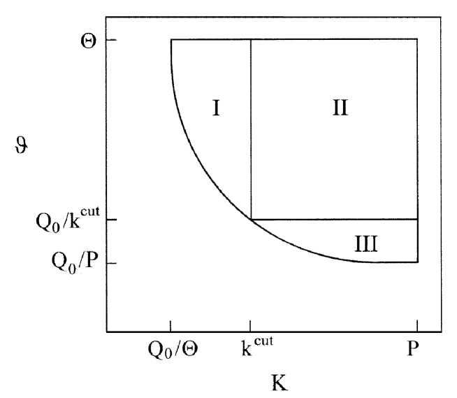
Figure 2:

Figure 3:

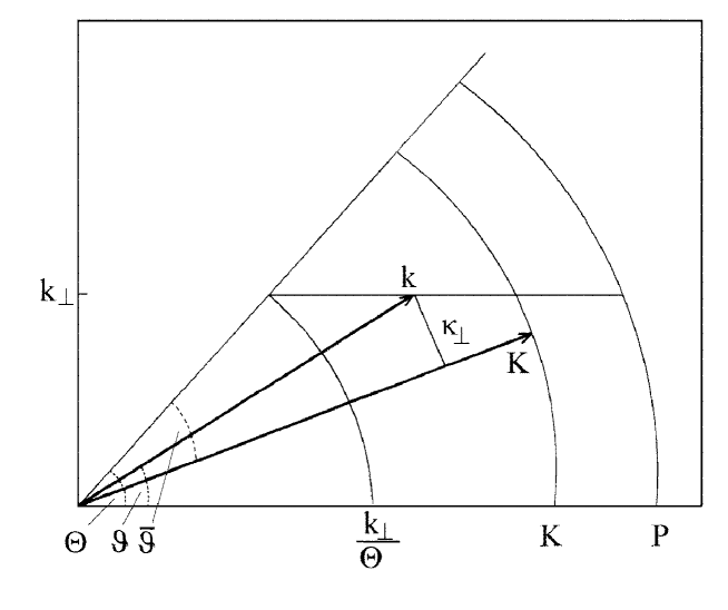
Figure 4:

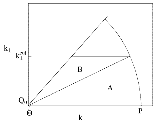
Figure 5:

$k_{\perp}^{\mathrm{c}ut}$ [GeV]

$k^{\mathrm{c}ut}$ [GeV]

Figure 6:

$k_{\perp}^{\mathrm{c}ut}$ [GeV]

$k^{\mathrm{c}ut}$ [GeV]

Figure 7:

$k_{\perp}^{\mathrm{c}ut}$ [GeV]

$k^{\mathrm{c}ut}$ [GeV]

Figure 8:

References

- [1] A.M. Polyakov, Sov. Phys. JETP, 32 (1971) 296; 33 (1971) 850.
- [2] K. Konishi, A. Ukawa and G. Veneziano, Nucl. Phys. B157 (1979) 45.
- [3] A. Bassetto, M. Ciafaloni, G. Marchesini, Nucl. Phys. B163 (1980) 477.
- [4] Yu. L. Dokshitzer, V. S. Fadin and V. A. Khoze, Z. Phys. C15 (1982) 325, C18 (1983) 37.
- [5] E. D. Malaza, B. R. Webber, Phys. Lett. 149B (1984) 501; Nucl. Phys. B267 (1986) 702.
- [6] I. M. Dremin, Phys. Lett. B313 (1993) 209.
- [7] Z. Koba, H.B. Nielsen and P. Olesen, Nucl. Phys. B40 (1972) 317.
-
[8]
B. I. Ermolayev and V. S. Fadin, JETP. Lett. 33 (1981) 285;
A. H. Mueller, Phys. Lett. 104B (1981) 161. - [9] Ya. I. Azimov, Yu. L. Dokshitzer, V. A. Khoze and S. I. Troyan, Z. Phys., C27 (1985) 65 and C31 (1986) 213.
-
[10]
V. A. Khoze, S. Lupia and W. Ochs, Phys. Lett. B394 (1997) 179;
“Perturbative Universality in Soft Particle Production”, preprint hep-ph/9711392, to appear in Eur. Phys. Journ. C. - [11] V.A. Khoze and W. Ochs, Int. J. Mod. Phys. A12 (1997) 2949.
- [12] E.A. De Wolf, I.M. Dremin and W. Kittel, Phys. Rep. 270 (1996) 1.
-
[13]
Yu.L. Dokshitzer, V.A. Khoze, A.H. Mueller and S.I. Troyan,
Rev. Mod. Phys. 60 (1988) 373;
“Basics of Perturbative QCD”, ed. J. Tran Thanh Van, Editions Frontières, Gif-sur-Yvette, 1991. - [14] W. Ochs and J. Wosiek, Phys. Lett. B304 (1993) 144; Z. Phys. C68 (1995) 269.
- [15] P. Carruthers, H.C. Eggers and I. Sarcevic, Phys. Lett. B254 (1991) 258; P. Carruthers and I. Sarcevic, Phys. Rev. Lett. 63 (1989) 1562.
- [16] E.A. De Wolf, Acta. Phys. Pol. B21 (1990) 611.
- [17] Yu. L. Dokshitzer and I. Dremin, Nucl. Phys. B402 (1993) 139.
- [18] Ph. Brax, J.L. Meunier and R. Peschanski, Z. Phys. C62 (1994) 649.
- [19] L. Lönnblad, Comp. Phys. Comm. 71 (1992) 15.
- [20] S. Lupia and W. Ochs, Phys. Lett. B418 (1998) 214.
- [21] OPAL Coll., K. Ackerstaff et al., Eur. Phys. Journ. C1 (1998) 479.
-
[22]
H.-J. Behrends et al., CELLO Coll., Phys. Lett. B256 (1991) 97;
I. Derado et al., Z. Phys. C47 (1990) 23, Z. Phys. C54 (1992) 357.