Dimensionally regularized study of nonperturbative
quenched QED

Abstract

We study the dimensionally regularized fermion propagator Dyson-Schwinger equation in quenched nonperturbative QED in an arbitrary covariant gauge. The nonperturbative fermion propagator is solved in $D\equiv 4-2\epsilon<4$ dimensional Euclidean space for a large number of values of $\epsilon$. Results for $D=4$ are then obtained by extrapolation to $\epsilon\to 0$. The nonperturbative renormalization is performed numerically, yielding finite results for all renormalized quantities. This demonstrates, apparently for the first time, that it is possible to successfully implement nonperturbative renormalization of Dyson-Schwinger equations within a gauge invariant regularization scheme such as dimensional regularization. Here we present results using the Curtis-Penningon fermion-photon proper vertex for two values of the coupling, namely $\alpha=0.6$ and $\alpha=1.5$ and compare these to previous studies employing a modified ultraviolet cut-off regularization. The results using the two different regularizations are found to agree to within the numerical precision of the present calculations.

I Introduction

Strong coupling quantum electrodynamics (QED) has been extensively studied through the use of the Dyson-Schwinger equations (DSE) [2, 3, 4]. In such studies it is unavoidable that the infinite set of coupled integral equations be truncated to those involving Green functions with relatively few external legs. This truncation has the consequence that one or more of the Green functions appearing in the remaining equations are no longer determined self-consistently by the DSE’s and so must be constrained, for example, by known symmetries (including Ward-Takahashi identities (WTI) [5]), the absence of artificial kinematic singularities, the requirements of multiplicative renormalizability (MR), and must be in agreement with perturbation theory in the weak coupling limit. Furthermore the gauge dependence of the resulting fermion propagator should eventually be ensured to be consistent with the Landau-Khalatnikov transformation [6].

What makes QED a particularly attractive theory to study with DSE techniques is that the coupled integral equations determining the photon and fermion propagators are completely closed once the photon-fermion proper vertex is specified. Up to transverse parts this proper vertex is in turn determined in terms of the fermion propagator by the corresponding WTI. Thus, the state of the art for this type of calculation consists of imposing the greatest possible set of constraints and constructing the most reasonable possible Ansatz for the transverse part of the vertex. While such a DSE approach to nonperturbative QED can never be an entirely first-principles approach, such as a lattice gauge theory treatment [7], it has the advantages that it is at times possible to obtain some analytical insights, there is no limit to the momentum range that can be studied and one is able to compare different regularization schemes. This latter property will be made use of in this paper.

A number of discussions of the choice of the transverse part of the proper vertex can be found in the literature, e.g., Refs. [8, 9, 10, 11, 12, 13, 14, 15, 16]. We will concentrate here on the Curtis-Pennington (CP) vertex [9, 10, 11, 12, 17], which satisfies both the WTI and the the constraints of multiplicative renormalizability. With a bare vertex (which breaks both gauge invariance and MR) the critical coupling of quenched QED differs by approximately 50% when calculated in the Feynman and Landau gauge. This should be compared to a difference of less than 2% for these gauges when calculated with the Curtis-Pennington vertex [12]. Even with the CP vertex, the variation is significantly greater for covariant gauge choices outside this range, particularly for negative gauges [17]. Extensions of this work to include nonperturbative renormalization were first performed numerically in Refs. [18, 19, 20]. In these latter works an obvious gauge covariance violating term, arising from the use of cut-off regularization and present in [12, 17] was omitted (see Refs. [13, 19] for a discussion of this). Without the gauge covariance violating term the variation of the critical coupling near the Landau gauge was again found to be rather small (less than 3% when going from Landau gauge to $\xi=$0.5 [19]).

Clearly, the gauge dependence of the (physical) critical coupling is decreased, but not eliminated, through the use of a photon-fermion proper vertex which satisfies the WTI. In other words, the choice of a vertex satisfying the WTI is a necessary but not sufficient condition in order to ensure the full gauge covariance of the Green functions of the theory and the gauge invariance of physical observables. The question that arises is whether the remaining gauge dependence in the critical coupling is primarily due to limitations of the vertex itself or whether it is due to the use of a UV cut-off regulator in these calculations.

Bashir and Pennington [14, 15] have pursued the first of these alternatives and have obtained, within a cut-off regularized theory, further restrictions on the transverse part of the vertex which ensure by construction that the critical coupling indeed becomes strictly gauge independent. It is not clear that adjusting the vertex to remove an unwanted gauge-dependence is the most appropriate procedure when using a gauge-invariance violating regularization scheme. It should be remembered that a cutoff in (Euclidean) momentum, apart from breaking Poincaré invariance, indeed also breaks gauge invariance. It is precisely because of this lack of gauge invariance that UV cut-off regulators have not been used in perturbative calculations in gauge theories for many years. Rather, the most common perturbative method of regularization in recent times has been that of dimensional regularization [21] where gauge invariance is explicitly maintained.

In this work we report on a DSE study of quenched nonperturbative QED using dimensional regularization in the renormalization procedure. Some early exploratory studies have been carried out in the past [22], but to our knowledge this work is the first complete nonperturbative demonstration of dimensional regularization and renormalization. Nonperturbative renormalization is performed numerically, in arbitrary covariant gauge, using the procedure first developed and applied in Refs. [18, 19, 20]. In these works the vertex used was that of Curtis and Pennington and so, as it is our aim to compare to previous results obtained with the use of cut-off regularization, we also use this vertex in the current work. In quenched QED there is no renormalization of the electron charge and the appropriate photon propagator is just the bare one. The resulting nonlinear integral equation for the fermion propagator is solved numerically in $D=4-2\epsilon<4$ Euclidean dimensional space. Successive calculations with decreasing $\epsilon$ are then extrapolated to $\epsilon=0$.

The organization of the paper is as follows: The renormalized and dimensionally regularized SDE formalism is discussed in Sec. II. This is followed by some representative numerical results in Sec. III. We present conclusions and an outlook in Sec. IV. An appendix details the final form of the fermion self-energy equations in $D$-dimensional Euclidean space.

II Formalism

In this section we provide a brief summary of the implementation of nonperturbative renormalization within the context of numerical DSE studies. We adopt a notation similar to that used in Refs. [18, 19, 20], to which the reader is referred for more detail. The formalism is presented in Minkowski space and the Wick rotation into Euclidean space can then be performed once the equations to be solved have been written down. It is important to note that although we use dimensional regularization, we can not make use of the popular perturbative renormalization schemes which are usually used in connection with this, such as $MS$ or $\overline{MS}$. The reason, of course, is that these schemes can only be defined in a purely perturbative context.

The renormalized inverse fermion propagator is defined through

$$S^{-1}(\mu;p)=A(\mu;p^{2})\not\!p-B(\mu;p^{2}) = Z_{2}(\mu,\epsilon)[\not\!p-m_{0}(\epsilon)]-\Sigma^{\prime}(\mu,\epsilon;p)$$ (1)

$$= \not\!p-m(\mu)-\widetilde{\Sigma}(\mu;p)\;\;\;,$$ (2)

where $\mu$ is the chosen renormalization scale, $m(\mu)$ is the value of the renormalized mass at $p^{2}=\mu^{2}$, $m_{0}(\epsilon)$ is the bare mass and $Z_{2}(\mu,\epsilon)$ is the wavefunction renormalization constant. Due to the WTI for the fermion-photon proper vertex, we have for the vertex renormalization constant $Z_{1}(\mu,\epsilon)=Z_{2}(\mu,\epsilon)$. The renormalized and unrenormalized fermion self-energies are denoted as $\widetilde{\Sigma}(\mu;p)$ and $\Sigma^{\prime}(\mu,\epsilon;p)$ respectively. These can be expressed in terms of Dirac and scalar pieces, where for example

$$\Sigma^{\prime}(\mu,\epsilon;p)=\Sigma^{\prime}_{d}(\mu,\epsilon;p^{2})\not\!p+\Sigma^{\prime}_{s}(\mu,\epsilon;p^{2})\;\;\;,$$ (3)

and similarly for $\widetilde{\Sigma}(\mu;p)$. We shall for notational brevity not explicitly indicate the dependence on $\epsilon$ of the renormalized quantities $A(\mu;p^{2})$, $B(\mu;p^{2})$ and $\widetilde{\Sigma}(\mu;p)$, since for these and other renormalized quantities we will always be interested in their $\epsilon\to 0$ limit. The renormalized mass function $M(p^{2})\equiv B(\mu;p^{2})/A(\mu;p^{2})$ is renormalization point independent, which follows straightforwardly from multiplicative renormalizability [19].

The renormalization point boundary condition

$$\left.S^{-1}(\mu;p)\right|_{p^{2}=\mu^{2}}=\not\!p-m(\mu)\>$$ (4)

implies that $A(\mu;\mu^{2})\equiv 1$ and $m(\mu)\equiv M(\mu^{2})$ and yields the following relations between renormalized and unrenormalized self-energies

$$\widetilde{\Sigma}_{d,s}(\mu;p^{2})=\Sigma^{\prime}_{d,s}(\mu,\epsilon;p^{2})-\Sigma^{\prime}_{d,s}(\mu,\epsilon;\mu^{2})\;\;\;.$$ (5)

Also, the wavefunction renormalization is given by

$$Z_{2}(\mu,\epsilon)=1+\Sigma^{\prime}_{d}(\mu,\epsilon;\mu^{2})$$ (6)

and the bare mass $m_{0}(\epsilon)$ is linked to the renormalized mass $m(\mu)$ through

$$m_{0}(\epsilon)=\left[m(\mu)-\Sigma^{\prime}_{s}(\mu,\epsilon;\mu^{2})\right]/Z_{2}(\mu,\epsilon)\;\;\;.$$ (7)

It also follows from MR that under a renormalization point transformation $\mu\to\mu^{\prime}$, $m(\mu^{\prime})=M({\mu^{\prime}}^{2})$ and $Z_{2}(\mu^{\prime},\epsilon)=A(\mu^{\prime};\mu^{2})\,Z_{2}(\mu,\epsilon)$ as discussed in Ref. [19].

The unrenormalized self-energy is given by the integral

$$\Sigma^{\prime}(\mu,\epsilon;p)=iZ_{1}(\mu,\epsilon)[e(\mu)\nu^{\epsilon}]^{2}\int\frac{d^{D}k}{(2\pi)^{D}}\gamma^{\lambda}{S}(\mu;k){\Gamma}^{\nu}(\mu;k,p){D}_{\lambda\nu}(\mu;p-k)\>,$$ (8)

where $\nu$ is an arbitrary mass scale introduced in $D$ dimensions so that the renormalized coupling $e(\mu)$ remains dimensionless. Since we are here working in the quenched approximation we have $Z_{3}(\mu,\epsilon)=1$, $e_{0}\equiv e(\mu)$, and the renormalized photon propagator ${D}^{\mu\nu}(\mu;q)$ is equal to the bare photon propagator

$$D^{\mu\nu}(q)=\left(-g^{\mu\nu}+\frac{q^{\mu}q^{\nu}}{q^{2}}-\xi\frac{q^{\mu}q^{\nu}}{q^{2}}\right)\frac{1}{q^{2}}\>$$ (9)

with $\xi$ being the covariant gauge parameter. Finally, ${\Gamma}^{\nu}(\mu;k,p)$ is the renormalized photon-fermion vertex for which we use the CP Ansatz, namely ($q\equiv k-p$)

$$\Gamma^{\mu}(\mu;k,p)=\Gamma_{\rm BC}^{\mu}(\mu;k,p)+\tau_{6}(\mu;k^{2},p^{2},q^{2})\left[\gamma^{\mu}(p^{2}-k^{2})+(p+k)^{\mu}{\not\!q}\right]\>,$$ (10)

where $\Gamma_{\rm BC}$ is the usual Ball-Chiu part of the vertex which saturates the Ward-Takahashi identity [8]

$$\Gamma^{\mu}_{\rm BC}(\mu;k,p) = \frac{1}{2}[A(\mu;k^{2})+A(\mu;p^{2})]\gamma^{\mu}$$ (12)

$$\hskip 28.45274pt+\frac{(k+p)^{\mu}}{k^{2}-p^{2}}\left\{[A(\mu;k^{2})-A(\mu;p^{2})]\frac{{\not\!k}+{\not\!p}}{2}-[B(\mu;k^{2})-B(\mu;p^{2})]\right\}$$

and the coefficient function $\tau_{6}$ is that chosen by Curtis and Pennington, i.e.,

$$\tau_{6}(\mu;k^{2},p^{2},q^{2})=-\frac{1}{2}[A(\mu;k^{2})-A(\mu;p^{2})]/d(k,p)\>,$$ (13)

where

$$d(k,p)=\frac{(k^{2}-p^{2})^{2}+[M^{2}(k^{2})+M^{2}(p^{2})]^{2}}{k^{2}+p^{2}}\>.$$ (14)

The unrenormalized scalar and Dirac self–energies are extracted out of the DSE, Eq. (8), by taking $\frac{1}{4}{\rm Tr}$ of this equation, multiplied by 1 and $\not\!p/p^{2}$, respectively. Note that we use the conventions of Muta [23]

$$\gamma^{\mu}\gamma_{\mu} = D\hskip 28.45274pt\Rightarrow\hskip 28.45274pt\gamma^{\mu}\gamma^{\nu}\gamma_{\mu}=(2-D)\gamma^{\nu}$$

$${\rm Tr}\left[\gamma^{\mu}\gamma^{\nu}\right] = 4g^{\mu\nu}\hskip 62.59596pt{\rm Tr}[{\bf 1}]\>=\>4$$

$$\hskip 62.59596ptg^{\mu}{}_{\mu}\>=\>D$$

for the Dirac algebra.

The integrands appearing in Eq. (8) only depend on the magnitude of the internal fermion’s momentum $k^{2}$ as well as the angle $\theta$ between the fermion and photon momentum. Hence the D-dimensional integrals reduce to 2-dimensional ones, i.e.,

$$\int d^{D}k\,f(k^{2},p^{2},k\cdot p)=\int d\Omega^{D-1}\times\int_{0}^{\infty}dk\,k^{D-1}\int_{0}^{\pi}d\theta\>\sin^{D-2}\theta\>f(k^{2},p^{2},k\cdot p)$$ (15)

where

$$\int d\Omega^{D}=\frac{2\pi^{D/2}}{\Gamma(D/2)}$$ (16)

is the surface area of a D-dimensional sphere. Furthermore, it is possible to express all the angular integrals in terms of a single hypergeometric function so that it is only necessary to do one integral numerically. The final form of the regularized self-energies is presented in the appendix.

The momentum integration is done numerically on a logarithmic grid and the renormalized fermion DSE solved by iteration. Note that the momentum integration extends to infinity, necessitating a change in integration variables. A convenient choice of transformation is

$$y=y_{\rm lo}\ \left(\frac{2}{1-t}\right)^{\frac{1}{\epsilon}}\;\;\;,$$ (17)

where $y_{\rm lo}$ is some lower integration bound and the integration variable $t$ ranges from $-1$ to $1$. The infinite range of the integration also requires an extrapolation of $A(\mu;p^{2})$ and $B(\mu;p^{2})$ above the highest gridpoint. We check insensitivity to this extrapolation by comparing results obtained with a number of different extrapolation prescriptions. In addition, we use grids which extend some 20-30 orders of magnitude beyond what is usually used in cut-off studies. In summary, we believe that we have verified that the effect of the extrapolation to infinity is well-controlled.

III Results

We present here solutions for the DSE for two values of the coupling $\alpha=e_{0}^{2}/4\pi$, namely $\alpha=0.6$ and $\alpha=1.5$. These were chosen so that they correspond to couplings respectively well below and above the critical coupling found in previous UV cut-off based studies. The gauge parameter is set at $\xi=0.25$, the renormalization point which we used is $\mu^{2}=10^{8}$ and the renormalized mass is taken to be $m(\mu)=400$. Note that all results are quoted in terms of dimensionless units, i.e., all mass and momentum scales can be simultaneously multiplied by any desired mass scale.

Figs. 1 and 2 show a family of solutions with the regulator parameter $\epsilon$ decreased from $0.08$ to $0.03$ for the two values of the coupling. We see that the mass function increases in strength in the infrared and tails off faster in the ultraviolet as $\epsilon$ is reduced or $\alpha$ is increased.

Furthermore, it is important to note the strong dependence on $\epsilon$, even though this parameter is already rather small. As one would expect, the ultraviolet is most sensitive to this regulator, however even in the infrared there is considerable dependence due to the intrinsic coupling between these regions by the renormalization procedure. This strong dependence on $\epsilon$ should be contrasted with the situation in cut-off based studies where it was observed that already at rather modest cut-offs ($\Lambda^{2}\approx 10^{10}$) the renormalized functions $A$ and $M$ had reached their asymptotic limits. At present it is not possible to decrease $\epsilon$ significantly below the values shown in Figs. 1 and 2 because of limitations due to numerical noise. In order to extract the values of $A$ and $M$ in four dimensions we therefore need to extrapolate to $\epsilon=0$. More sophisticated numerical techniques are being investigated and will hopefully allow explicit calculations at smaller $\epsilon$ values in the future.

An extrapolation such as this always involves an added uncertainty in the final result. It is fortunate that it is possible to estimate this uncertainty by making use of the fact that in the limit $\epsilon\rightarrow 0$ the renormalized quantities should become independent of the arbitrary scale $\nu$, which was introduced to keep the coupling $\alpha$ dimensionless in $D$ dimensions. In Fig. 3 we show $A(p^{2})$ and $M(p^{2})$ evaluated with $\alpha=e_{0}^{2}/4\pi=1.5$ in the infrared (at $p^{2}=1$) as a function of $\epsilon$ for a range of values of $\nu$. The results at $\epsilon=0$ are extracted from cubic polynomial fits in $\epsilon$. As may be observed, the agreement between the different curves at $\epsilon=0$ is excellent, being of the order of $0.2\%$.

In Fig. 4 we show the results extrapolated to $\epsilon=0$ as a function of the momentum (again for $\alpha=1.5$). Also shown, although hardly distinguishable, is the result for these curves as obtained in the modified UV cutoff based studies, which used a gauge-covariance fix to remove an obvious part of the gauge dependence induced by the cutoff [19]. Again the agreement is very good for a wide range in $p^{2}$ and $\nu$. Only in the ultraviolet region (above say $p^{2}=10^{12}$) do differences between the curves become discernible. We see in Fig. 4 that the UV cutoff result is almost indistinguishable from the $\nu=100$ result at essentially all momenta. The discrepancies for the $\nu=1$ and $10$ cases are greater in the UV due to the fact that in this region the errors introduced by the extrapolation procedure in $\epsilon$ become comparable (for a cubic fit) to the functions’ values there. This is supported by the following two observations. Firstly, from Fig. 3 we see that the $\epsilon$-dependence is almost linear for $\nu=100$, whereas it clearly deviates from linearity for the other cases. Secondly, there is little change in the $\nu=100$ extrapolation as we change the order of the fit polynomial up to order $\epsilon^{6}$, whereas the $\nu=1$ and $10$ results show greater variation. We conclude that the $\nu=100$ results in Fig. 3 provide the most reliable $\epsilon\to 0$ extrapolation. It should also be noted that the oscillatory behaviour in the mass function first noticed in [18] is reproduced in this work, and the results for the unmodified UV cutoff disagree with those from dimensional regularization.

Finally, we present in Tables I and II the bare mass $m_{0}(\epsilon)$ and the wavefunction renormalization for the two cases studied as a function of the regularization parameter $\epsilon$ and the gauge parameter $\xi$. It should be noted that these two quantities are by their very nature sensitive to the behaviour of $A(p^{2})$ and $B(p^{2})$ in the ultraviolet. In particular, while any renormalized quantities were found to have a negligible dependence on the precise form of the extrapolation of the integrands beyond the highest gridpoint, it was found that $Z_{2}(\mu,\epsilon)$ and $m_{0}(\epsilon)$ do show some small dependence ($<1\%$) in our calculations. The values for these quantities listed in Tables I and II were obtained by assuming a simple power-behaviour of the integrands beyond the highest gridpoint. As was seen in the UV cutoff studies, the wavefunction renormalization (for $\xi>0$) actually decreases as the regularization is removed. In the same way the behaviour of $Z_{2}$ as a function of the gauge parameter is qualitatively the same as observed in the cut-off studies, i.e. at fixed $\epsilon$ it decreases as one moves from the Landau towards the Feynman gauge. The bare mass $m_{0}$, on the other hand, appears to show a different behaviour to before, at least for large couplings: while in the present work it decreases as the gauge parameter is increased for all $\epsilon$, in cut-off studies it only did this for moderately small cut-offs. It is quite possible that this different qualitative behaviour reflects the fact the even the lowest $\epsilon$’s which have been reached here “correspond” to rather modest cut-offs. In connection with this note that at the values of $\epsilon$ shown in Tables I and II the mass functions in Figs. 1 and 2 are still positive everywhere, the oscillations only setting in as one extrapolates toward $\epsilon\rightarrow 0$.

TABLE I.: Renormalization constant $Z_{2}(\mu,\epsilon)$ and bare mass $m_{0}(\epsilon)$ as functions of regularization parameter $\epsilon$ for $\alpha=0.6$ in various gauges $\xi$. All solutions are with renormalization point $\mu^{2}=1.00\times 10^{8}$ and renormalized mass $m(\mu)=400.0$

$\epsilon$		$Z_{2}(\mu,\epsilon)$						$m_{0}(\epsilon)$
		$\xi=0$		$\xi=0.25$		$\xi=0.5$		$\xi=0$			$\xi=0.25$			$\xi=0.5$
0.	08	1.	000	0.	957	0.	917	2.	30 $\times$	$10^{2}$	2.	29 $\times$	$10^{2}$	2.	28 $\times$	$10^{2}$
0.	07	1.	000	0.	944	0.	891	1.	91 $\times$	$10^{2}$	1.	90 $\times$	$10^{2}$	1.	89 $\times$	$10^{2}$
0.	06	1.	000	0.	924	0.	854	1.	46 $\times$	$10^{2}$	1.	45 $\times$	$10^{2}$	1.	44 $\times$	$10^{2}$
0.	05	1.	000	0.	896	0.	802	9.	75 $\times$	$10^{1}$	9.	66 $\times$	$10^{1}$	9.	57 $\times$	$10^{1}$
0.	04	1.	000	0.	851	0.	725	5.	07 $\times$	$10^{1}$	5.	00 $\times$	$10^{1}$	4.	94 $\times$	$10^{1}$
0.	03	1.	000	0.	779	0.	606	1.	59 $\times$	$10^{1}$	1.	56 $\times$	$10^{1}$	1.	53 $\times$	$10^{1}$

TABLE II.: As above, but for $\alpha=1.5$

$\epsilon$		$Z_{2}(\mu,\epsilon)$						$m_{0}(\epsilon)$
		$\xi=0$		$\xi=0.25$		$\xi=0.5$		$\xi=0$			$\xi=0.25$			$\xi=0.5$
0.	08	1.	000	0.	897	0.	805	9.	20 $\times$	$10^{1}$	9.	06 $\times$	$10^{1}$	8.	92 $\times$	$10^{1}$
0.	07	1.	000	0.	865	0.	749	5.	51 $\times$	$10^{1}$	5.	40 $\times$	$10^{1}$	5.	28 $\times$	$10^{1}$
0.	06	1.	000	0.	821	0.	674	2.	58 $\times$	$10^{1}$	2.	51 $\times$	$10^{1}$	2.	44 $\times$	$10^{1}$
0.	05	1.	000	0.	759	0.	576	7.	94 $\times$	$10^{0}$	7.	60 $\times$	$10^{0}$	7.	28 $\times$	$10^{0}$
0.	04	1.	000	0.	669	0.	447	1.	10 $\times$	$10^{0}$	1.	02 $\times$	$10^{0}$	9.	54 $\times$	$10^{-1}$
0.	03	1.	000	0.	535	0.	286	2.	63 $\times$	$10^{-2}$	2.	27 $\times$	$10^{-2}$	1.	96 $\times$	$10^{-2}$

IV Conclusions and Outlook

We have reported here the first detailed study of the numerical renormalization of the fermion Dyson-Schwinger equation of QED through the use of a dimensional regulator rather than a gauge invariance-violating UV cut-off. The initial results presented here are encouraging. Firstly, we have explicitly demonstrated that the approach works and is independent of the intermediate dimensional regularization scale ($\nu$) as expected. Secondly, we have seen the interesting result that our calculations using dimensional regularization agree with modified UV cut-off calculations within the current numerical precision, but disagree with the unmodified UV cutoff ones.

A significant practical difference between the dimensionally and UV cut-off regularized approaches is that in the former it is at present necessary to perform an explicit extrapolation to $\epsilon=0$ whereas in the latter it was found that for a sufficiently large choice of UV cut-off the results became independent of the cut-off. This need to extrapolate, together with the high precision that one needs to attain in order to make meaningful comparisons with cut-off based studies, makes numerical dimensional regularization and renormalization of Schwinger-Dyson equations a rather formidable task. Nevertheless, although we are presently investigating whether it is numerically possible to extend the studies to even smaller values of $\epsilon$ in order to improve the precision of the $\epsilon\to 0$ extrapolation, the extrapolation to $\epsilon=0$ appears to be well under control, at least for values of the fermion momentum away from the ultraviolet region.

Having demonstrated the numerical procedure of renormalization using dimensional regularization, we now plan to study chiral symmetry breaking and in particular hope to extract the critical coupling as a function of the gauge parameter. Results of this ongoing work will be presented elsewhere. The eventual aim is to extend this treatment to the case of unquenched QED and to a systematic study of electron-photon proper vertices.

A Final form for the regularized fermion self-energies

In the quenched approximation, all angular integrals in the Dirac and scalar regularized self-energies defined by the Euclidean analogue of Eq. (8) may be expressed in terms of the integrals

$$I_{n}^{D}(w)={\Gamma\left({D\over 2}\right)\over\Gamma\left({D-1\over 2}\right)\sqrt{\pi}}\int_{0}^{\pi}d\theta\,\left({x+y\over z}\right)^{n}\,\sin^{D-2}\theta\,\quad\text{for }n=-1,1,2$$ (A1)

where we have defined dimensionless quantities $x=p^{2}/\nu^{2}$, $y=k^{2}/\nu^{2}$, $z=q^{2}/\nu^{2}=x+y-2\sqrt{xy}\cos\theta$ and $w$=$y/x$. Similarily, we shall for convenience define dimensionless versions of $A(\mu^{2};p^{2})$ and $B(\mu^{2};p^{2})$, namely $a(x)=A(\mu^{2};p^{2})$ and $\nu b(x)=B(\mu^{2};p^{2})$ (we suppress the dependence on $\mu$ here in order to make the notation less cumbersome). Explicit evaluation (for $0\leq w\leq 1$) yields

$$I_{-1}^{D}(w) = 1$$ (A2)

$$I_{1}^{D}(w) = (1+w)\,\,{}_{2}F_{1}(1,\epsilon;2-\epsilon;w)$$ (A3)

$$I_{2}^{D}(w) = 2\left({1+w\over 1-w}\right)^{2}\left(-{1-2\epsilon\over 2}I^{D}_{1}(w)+1-\epsilon\right)\,,$$ (A4)

and for $w\geq 1$ one may use

$$I_{n}^{D}(w)=I_{n}^{D}(w^{-1})\;\;\;.$$ (A5)

Defining

$$\widetilde{d_{E}}(x,y) = \frac{d_{E}(x,y)}{x+y}$$ (A6)

$$\widetilde{\Delta{a}}(x,y) = \frac{a(x)-a(y)}{(1-w)/(1+w)}$$ (A7)

(and similarly for $\widetilde{\Delta{b}}(x,y)$) the regularized self-energies in the quenched approximation become

$$\Sigma^{\prime}_{d}(\mu,\epsilon;x) = \frac{\alpha_{0}}{4\pi}(4\pi)^{\epsilon}\frac{Z_{1}(\mu,\epsilon)}{\Gamma(2-\epsilon)}\int_{0}^{\infty}dy\frac{y^{-\epsilon}}{ya^{2}(y)+b^{2}(y)}\,w$$ (A8)

$$\times \Bigg{\{}a(y)\frac{a(x)+a(y)}{2}\xi\left(1-\epsilon\right)\left(1-I_{1}^{D}(w)\right)$$ (A12)

$$+a(y)\frac{\widetilde{\Delta a}(x,y)}{2}\left[\Bigl{(}{1\over 2}+\left(1-\xi\right)\left(1-\epsilon\right)-{3-2\epsilon\over 2\tilde{d}_{E}(x,y)}\left(\frac{1-w}{1+w}\right)^{2}\Bigr{)}\left(I_{1}^{D}(w)-1\right)\right.$$

$$\left.\hskip 142.26378pt+\frac{2\xi w}{(1+w)^{2}}I_{1}^{D}(w)\right]$$

$$+\frac{b(y)}{x+y}\widetilde{\Delta b}(x,y)\left[\Bigl{(}{1\over 2}+\left(1-\xi\right)\left(1-\epsilon\right)\Bigr{)}\left(I_{1}^{D}(w)-1\right)+\frac{\xi}{1+w}I_{1}^{D}(w)\right]\Bigg{\}}$$

and

$$\Sigma^{\prime}_{s}(\mu,\epsilon;x) = \frac{\alpha_{0}}{4\pi}(4\pi)^{\epsilon}\frac{Z_{1}(\mu,\epsilon)}{\Gamma(2-\epsilon)}\int_{0}^{\infty}dy\frac{y^{1-\epsilon}}{ya^{2}(y)+b^{2}(y)}\frac{1}{x(1+w)}$$ (A13)

$$\times \Bigg{\{}b(y)\frac{a(x)+a(y)}{2}\left(3-2\epsilon+\xi\right)I_{1}^{D}(w)$$ (A17)

$$-a(y)\widetilde{\Delta b}(x,y)\left[\Bigl{(}{1\over 2}+\left(1-\xi\right)\left(1-\epsilon\right)\Bigr{)}\left(I_{1}^{D}(w)-1\right)+\frac{\xi w}{1+w}I_{1}^{D}(w)\right]$$

$$+b(y)\widetilde{\Delta a}(x,y)\left[\Bigl{(}{1\over 2}+\left(1-\xi\right)\left(1-\epsilon\right)\Bigr{)}\left(I_{1}^{D}(w)-1\right)\right.$$

$$\left.\hskip 142.26378pt+\left(\frac{\xi}{2}+\frac{3-2\epsilon}{2\widetilde{d_{E}}(x,y)}\left(\frac{1-w}{1+w}\right)^{2}\right)I_{1}^{D}(w)\right]\Bigg{\}}$$

It should be remembered that the equivalent expressions in cut-off regularized quenched QED suffer from an ambiguity due to the lack of gauge invariance in those calculations: one obtains different results at this stage depending one whether or not one has made use of the Ward-Takahashi identity in the initial stages of the calculation[13, 14]. The difference shows up in the terms multiplied by $a^{2}(y)$ and $b^{2}(y)$. Readers may readily convince themselves that no such ambiguity exists in the present work. In order to do this, the following identity is of use:

$$0\>=\>\int_{0}^{\infty}dy\,y^{1-\epsilon}\left(2{1-\epsilon\over y-x}\>+\>\left[{2\epsilon-1\over y-x}-{1\over x+y}\right]I_{1}^{D}(w)\right)$$ (A18)

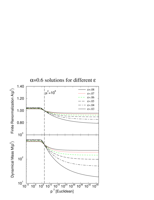
FIG. 1.: The finite renormalization $A(p^{2})$ and mass function $M(p^{2})$ for various choices of the regulator parameter $\epsilon$. These results have coupling $\alpha=0.6$, gauge parameter $\xi=0.25$, renormalization point $\mu^{2}=10^{8}$, renormalized mass $m(\mu)=400$ and scale $\nu=1$. In the low $p^{2}$ region the smallest $\epsilon$ has the largest value of $M(p^{2})$.

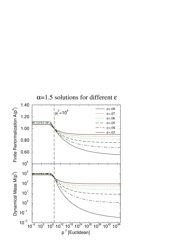
FIG. 2.: Same as Fig. 1 for $\alpha=1.5$

FIG. 3.: The finite renormalization $A(p^{2})$ and mass function $M(p^{2})$ evaluated at $p^{2}=1$ for various values of the regulator parameter $\epsilon$ and extrapolated to $\epsilon=0$ by fitting a polynomial cubic in $\epsilon$. Shown are results for three scales $\nu=1$, $10$ and $100$. All other parameters are those of Fig. 2. The different scales coincide at $\epsilon=0$ to an accuracy of approximately $0.2\%$.

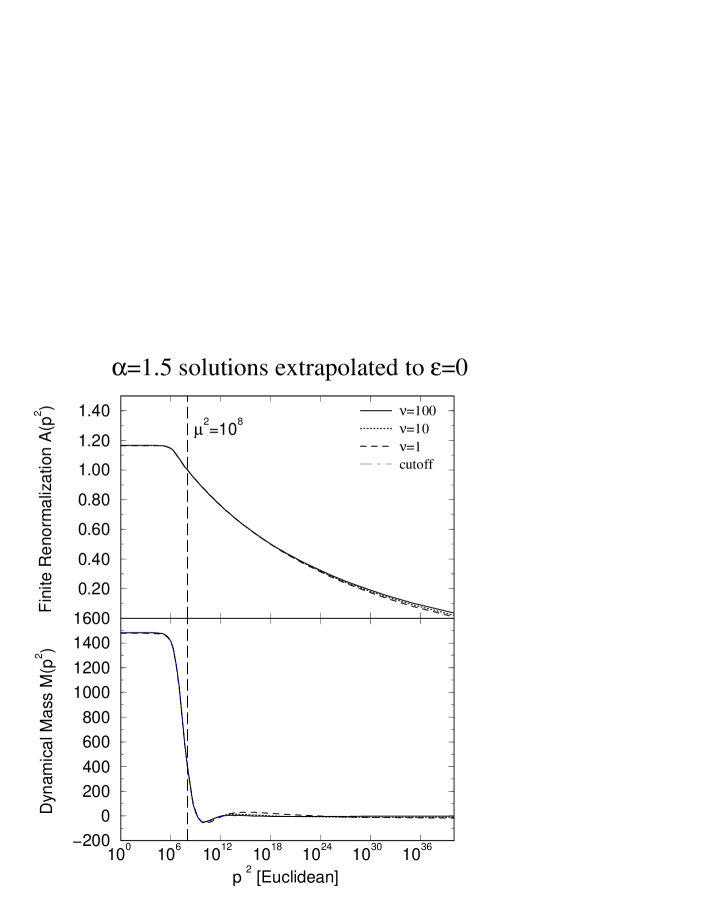
FIG. 4.: The finite renormalization $A(p^{2})$ and mass function $M(p^{2})$ extrapolated to $\epsilon=0$ at every momentum point for three different scales $\nu=1$, $10$ and $100$. They were calculated by fitting a cubic polynomial in $\epsilon$ at each momentum point. All other parameters are those of Fig. 2. Also shown is the result obtained using a modified UV cutoff. The UV cutoff and extrapolated $\nu=100$ results are indistinguishable in these plots.

REFERENCES

- [1] Email addresses: aschreib@physics.adelaide.edu.au, tsizer@physics.adelaide.edu.au, awilliam@physics.adelaide.edu.au.
- [2] C.D. Roberts and A.G. Williams, Dyson-Schwinger Equations and their Application to Hadronic Physics, in Progress in Particle and Nuclear Physics, Vol. 33 (Pergamon Press, Oxford, 1994), p. 477.
- [3] V. A. Miranskii, Dynamical Symmetry Breaking in Quantum Field Theories, (World Scientific, Singapore, 1993).
- [4] P. I. Fomin, V. P. Gusynin, V. A. Miransky and Yu. A. Sitenko, Riv. Nuovo Cim. 6, 1 (1983).
- [5] J.C. Ward, Phys. Rev. 78, 124 (1950); Y. Takahashi, Nuovo Cimento 6, 370 (1957).
- [6] L. D. Landau and I. M. Khalatnikov, Sov. Phys. JETP 2, 69 (1956) [translation of Zhur. Eksptl. i Teoret. Fiz. 29, 89 (1955)]; K. Johnson and B. Zumino, Phys. Rev. Lett. 3, 351 (1959).
- [7] H.J. Rothe, Lattice Gauge Theories: an Introduction, (World Scientific, Singapore, 1992).
- [8] J.S. Ball and T.W. Chiu, Phys. Rev. D 22, 2542 (1980); ibid., 2550 (1980).
- [9] D.C. Curtis and M.R. Pennington, Phys. Rev. D 42, 4165 (1990).
- [10] D.C. Curtis and M.R. Pennington, Phys. Rev. D 44, 536 (1991).
- [11] D.C. Curtis and M.R. Pennington, Phys. Rev. D 46, 2663 (1992); ibid., D 47, 1729 (1993).
- [12] D.C. Curtis and M.R. Pennington, Phys. Rev. D 48, 4933 (1993).
- [13] Z. Dong, H. Munczek, and C.D. Roberts, Phys. Lett. 333B, 536 (1994).
- [14] A. Bashir and M. R. Pennington, Phys. Rev. D 50, 7679 (1994).
- [15] A. Bashir and M. R. Pennington, Phys. Rev. D 53, 4694 (1996).
- [16] A. Kızılersü, M. Reenders, and M. R. Pennington, Phys. Rev. D 52, 1242 (1995).
- [17] D. Atkinson, J.C.R. Bloch, V.P. Gusynin, M. R. Pennington, and M. Reenders, Phys. Lett. 329B, 117 (1994).
- [18] F.T. Hawes and A.G. Williams, Phys. Rev. D 51, 3081 (1995).
- [19] F.T. Hawes, A.G. Williams and C.D. Roberts, Phys. Rev. D 54, 5361 (1996).
- [20] F.T. Hawes, T. Sizer and A.G. Williams, Phys. Rev. D 55, 3866 (1997).
- [21] G. ’t Hooft and M.J.G. Veltman, Nucl. Phys. B44, 189 (1972).
- [22] L. von Smekal, P. A. Amundsen, and R. Alkofer, Nucl. Phys. A529, 633 (1991); M. Becker, “Nichtperturbative Strukturuntersuchungen der QED mittels genäherter Schwinger-Dyson-Gleichungen in Dimensioneller Regularisierung”, Ph.D. dissertation, W. W. U. Münster,1995.
- [23] T. Muta, Foundations of quantum chromodynamics – An introduction to perturbative methods in gauge theories, (World Scientific, Singapore, 1987).