TAUP 2493-97
PRECISE ESTIMATES OF HIGH ORDERS IN QCD

Abstract

I review the recent work on obtaining precise estimates of higher-order corrections in QCD and field theory.

1 Introduction

The precision of the experimental data on electroweak interactions and QCD is now very high and it is expected to become significantly higher within the next few years. This has triggered a substantial refinement in the corresponding theoretical calculations. Yet, already now for certain experimental quantities the theoretical uncertainty is one of the major open questions in the interpretation of the data and in the search for signals of physics beyond the Standard Model. A striking example is the need for a precise determination of the gauge couplings at the weak scale, which is the prerequisite for investigation of possible unification of couplings at some GUT scale.

One of the reasons for this current state of affairs in the relation between the theory and experiment is that computation of high orders in perturbation theory for quantum field theories, and especially non-abelian gauge theories in $3{+}1$ dimensions is extremely hard. State-of-the-art calculations available today for this kind of theories have reached, after a very large effort, the 3-rd and the 4-th order in $\alpha_{s}$, for observables and for the $\beta$-function, respectively [high_orders, beta4loop, massAnDim]. Without a major breakthrough in the relevant techniques it is unlikely that exact results for the next order will become available in the foreseeable future. Moreover, even if explicit expressions for very high order terms do become available, we still have to deal with the fact that the perturbative series of interest are asymptotic, with zero radius of convergence and usually are not even Borel summable. In this talk I will review an approach which has been recently suggested to deal with some of these problems.

2 Perturbation Theory: Diseases and a Promising Therapy

As mentioned in the Introduction, the perturbation series in QCD is expected to be asymptotic with rapidly growing coefficients:

$$S(x)=\sum^{\infty}_{n=0}c_{n}x^{n}~{},\quad x\equiv\frac{\alpha_{s}}{\pi}~{},\qquad c_{n}\simeq n!K^{n}{n}^{\gamma}$$ (1)

for some coefficients $K,\gamma$ [renmvz, RenormRev]. Anyone who wants to make use of QCD perturbation theory to carry out precision analysis of observables has to face several practical problems:

• only few first orders in (1) are known for any observable ($n\leq 3$)

• the series has zero radius of convergence

• the series is usually not Borel summable. Borel summation is a trick that sometimes works for summing series with factorial divergence. Consider the series for $S(x)$ in eq. (1). We can define a new function, ${\cal S}(y)$, whose series is obtained from (1) by dividing the $n$-th term by $n!$,

  $${\cal S}(y)=\sum^{\infty}_{n=0}\left({c_{n}\over n!}\right)y^{n}$$ (2)

  If the new series is convergent, the original function $S(x)$ can be obtained by the so-called inverse Borel transform,

  $$S(x)={1\over x}\,\int_{0}^{\infty}e^{{-}y/x}{\cal S}(y)dy$$ (3)

  provided ${\cal S}(y)$ has no singularities along the integration path.

  

  Unfortunately, in QCD it is known that for a generic observable ${\cal S}(y)$ has poles on both the positive and negative $y$ axis in the complex $y$ plane. These are usually referred to as infrared and ultraviolet renormalons, respectively. The figure to the left shows a schematic description of poles in the Borel transform of a generic series for a QCD observable.

  The presence of singularities along the integration path makes the integral (3) ill-defined. One can try to define it by going around the poles, but this introduces an ambiguity proportional to the pole residue, since different deformations of the integration path will give different results.

• renormalization scale dependence: finite-order perturbative predictions depend on the arbitrary renormalization scale $\mu$ through the coupling, $\alpha_{s}=\alpha_{s}(\mu)$. This renormalization scale is most pronounced at leading order in perturbation theory and decreases with the inclusion of higher order terms.

• renormalization scheme dependence: in principle, the theory can be renormalized in any valid renormalization scheme, yielding the same predictions for any physical observable. In practice, when we work with a finite number of perturbative terms, the results depend on the renormalization scheme.

There is no “miracle cure” which would solve these problems completely. However, we should and can minimize their effect. Thus the practical issue is how to get the best possible precision, given a fixed number of terms in the perturbative expansion. In the following, I will discuss one method which has already shown considerable progress towards this goal. The method is based on the so-called Padé Approximants (PA-s) [PadeInQFT]-[EJJKS].

3 Padé to the Rescue

Padé Approximants [Baker, BenderOrszag] are rational functions chosen to have a Taylor expansion equal the perturbative series to the order calculated. Given a series

$$S(x)=c_{0}+c_{1}x+c_{2}x^{2}+c_{3}x^{3}+\cdots+c_{N}x^{N}+\,{\cal O}(x^{N+1})$$ (4)

one can always find a rational function

$$[L/M]\equiv\frac{a_{0}+a_{1}x+...+a_{L}x^{L}}{1+b_{1}x+...+b_{M}x^{M}}~{}:\qquad L+M=N$$ (5)

such that $[L/M]$ has the Taylor series

$$[L/M]=c_{0}+c_{1}x+c_{2}x^{2}+c_{3}x^{3}+\cdots+c_{N}x^{N}+\,\tilde{c}_{N+1}x^{N+1}+\cdots$$ (6)

The rational function in (5) is called the $[L/M]$ Padé Approximant.

It is important to keep in mind that at a given finite order in $x$ the $[L/M]$ Padé in (5) is formally as valid representation of $S(x)$ as the original perturbation expansion. Moreover, in practice the PA-s turn out to posses many important and useful properties which are absent in the straightforward perturbation theory.

Thus, even though PA is constructed to reproduce the series (4) only up to order $N$, it turns out that under rather mild conditions the next term in the Taylor expansion of the PA in eq. (6), $\tilde{c}_{N+1}$, provides a good estimate, $c^{est}_{N+1}=\tilde{c}_{N+1}$. We call it the Pade Approximant Prediction (PAP), of the next coefficient $c_{N+1}$ in the series (4):

$$\left|\frac{c^{est}_{N+1}}{c_{N+1}}-1\right|\ll 1$$ (7)

and for sufficiently large $N$ the relative error decays exponentially fast,

$$\left|\frac{c^{est}_{N+1}}{c_{N+1}}-1\right|\sim e^{-\sigma N}\,,\qquad\sigma=\hbox{const}$$ (8)

Let us consider some simple examples, starting with the trivial case of a single-pole geometric series

$$\frac{A}{1-Bx}=\sum_{n=0}^{\infty}c_{n}x^{n}$$ (9)

It is easy to convince oneself that in this case the $[L/M]$ Padé is exact for $L\geq 0$, $M\geq 1$. For example, if we attempt to construct a [10/10] Padé of (9), we will find that the a priori 10-th degree polynomials in numerator and denominator reduce to a degenerate case of a constant and 1-st degree polynomial, respectively,

$$[10/10]\equiv\frac{P_{10}(x)}{Q_{10}(x)}=\frac{A}{1-Bx}$$ (10)

Once this is clear, the extension to a sum of finite number of poles in obvious,

$$\sum_{i=1}^{K}\frac{A_{i}}{1-B_{i}x}=\sum_{n=0}^{\infty}c_{n}x^{n}\qquad\Longrightarrow\qquad[L/M]\hbox{\ exact for\ }\,L\geq K-1,\ M\geq K$$ (11)

One can also show that for an infinite number of isolated poles, i.e. when $f(x)=\displaystyle\sum_{0}^{\infty}c_{n}x^{n}$ is a meromorphic function, the sequence of $[L/L+k]$ for $k$ fixed converges to $f(x)$ as $L\rightarrow\infty$,

$$[L/L+k]\,\,\mathop{\hbox to27.0pt{\rightarrowfill}}_{L\rightarrow\infty}\,\,f(x)\,;\qquad\,k=0,\pm 1,\pm 2,\dots$$ (12)

A somewhat less intuitive, but very important result is that in certain cases the Padé sequence $[L/L+k]$ converges exponentially fast in $L$ to the correct function even for a factorially divergent asymptotic series with zero radius of convergence. A classical example [BenderOrszag] is the function

$$g(x)=\int_{0}^{\infty}\frac{e^{-t}}{1+xt}\,dt=\sum_{0}^{\infty}(-x)^{n}\,n!$$ (13)

Here again it turns out that $[L/L+k]\,\longrightarrow\,g(x)$ as $L\rightarrow\infty$.

The crucial property of the series in (13) which makes this possible is that it has alternating signs. It is easy to show that this implies that all the poles of the Borel transform of (13) are on the negative real axis, and hence that the series is Borel summable. More generally, when the series is Borel summable, Padé will converge to the correct result.

It is interesting to note that the exponentially fast convergence of PA-s is not limited to meromorphic functions. As a simple example, consider the hypergeometric function $F({-}{1\over 2},{3\over 2},1,x)$ [Abramowitz], which has a cut for $x\geq 1$. Fig. 1 shows that despite the cut, the diagonal PA-s evaluated at $x=0.2$ converge exponentially fast.

Fig. 1: Exponentially fast convergence of Padé despite the presence of a cut: relative error of diagonal [L/L] Padé for the hypergeometric function $F(-1/2,3/2,1,x)$ which has a cut for $x\geq 1$. The Padé is evaluated to the left of the cut, at $x=0.2$.

4 Applications to Quantum Field Theory

While such mathematical examples are instructive, in order to gain confidence in the method, we need to see how it fares on high-order series taken from quantum field theory. As the first test case, we consider the scalar field theory with Gaussian propagators. High-order perturbation expansions of Green’s functions in this theory have been computed in Ref. [Bervillier]. Fig. 2 demonstrates the convergence of PAP for the relevant coefficients for the 4-point Green’s function in $D=4$ [phi4PAP]. The relative error is $\sim 10^{-3}$ at 5-th order. For comparison also shown are relative errors of estimates based on asymptotic behavior of large orders in perturbation theory, as given in [phi4PAP]. Clearly, at 5-th order Padé does better by about 4 orders of magnitude.

Fig. 2: Padé predictions (crosses) for high-order terms in the perturbative expansion for 4-point Green’s function in a scalar field theory in $D=4$. For comparison also included are predictions based on asymptotic large-order behavior (circles).

If information is available about the asymptotic behavior of $c_{n}$, it is possible to obtain an explicit expression for the the error formula on the r.h.s. of (8). For example, we have demonstrated that if

$$\epsilon_{n}\equiv\frac{c_{n}\,c_{n+2}}{c^{2}_{n+1}}-1\,\simeq\,{1\over n},$$ (14)

as is the case for any series dominated by a finite number of renormalon singularities, then $\delta_{[L/M]}$ defined by

$$\delta_{[L/M]}\equiv\frac{c^{est.}_{L+M+1}-c_{L+M+1}}{c_{L+M+1}}$$ (15)

has the following asymptotic behaviour

$$\delta_{[L/M]}\simeq-\,\frac{M!}{K^{M}}\,,\quad~{}{\rm where}~{}K=L+M+a\,M$$ (16)

and where $a$ is a number of order 1 that depends on the series under consideration. For large $L,M$ eq. (16) yields an exponential decrease of the the error, as in eq. (8).

This prediction agrees very well with the known errors in the PAP’s [SEK] for the QCD vacuum polarization D function calculated in the large $N_{f}$ approximation [Dfunction], as seen in Fig. 3a.

One can repeat this exercise also for the Borel transform of the D function series. As mentioned earlier, a generic Borel transform is characterized by the presence of poles (more generally, branch points) on the real axis. In view of this, we expect an even faster convergence in this case, since the Padé, being a rational function, is particularly well-suited to reproduce this analytic structure. Indeed, it turns out that in this case $\epsilon_{n}\sim 1/n^{2}$ and

$$\delta_{[M/M]}\simeq-\,\frac{(M!)^{2}}{K^{2M}}$$ (17)

which agrees very well with the corresponding PAP results shown in Fig. 3b [SEK, Erice95].

The high degree of agreement between the analytical error estimates in eqs. (16) and (17) and the actual errors in PAP suggest that one can substantially improve the PAP method by systematically including the error estimates $\delta_{[L/M]}$ as a correction, yielding the Asymptotic Padé Approximant Predictions (APAPs):

$$c^{APAP}_{L+M+1}={c^{est}_{L+M+1}\over 1+\delta_{L+M+1}}$$ (18)

where $c^{est}_{L+M+1}$ is the original PAP prediction without the additional correction, as in eq. (15), and $\delta_{L+M+1}$ is obtained by fitting (16) to the known lower orders [EKSbeta].

Fig. 3: Relative errors in the $[L/M]$ Padé Approximant Predictions [SEK, Erice95] (a) for the QCD vacuum polarization D-function series, evaluated to all orders in the large-$N_{f}$ approximation [Dfunction] (the rate of convergence agrees with expectations for a series with a discrete set of Borel poles), and (b) for the Borel transform of the D-function series, where the convergence is particularly striking. The straight lines correspond to the exponential decay given by the respective error formulae, eqs. (16) and (17). The crosses, diamonds and squares correspond to $M=L+1,L+1,L$, respectively.

The APAP method results not only in a substantial improvement of the PAP estimates, but also significantly reduces the difference between the predictions based on different $[L/M]$ values at a given order, $L+M$=fixed.

The method has been applied to the Bjorken sum rule for the difference of first moments of proton and neutron structure functions $g_{1}(x,Q^{2})$ in polarized deep inelastic scattering [Bjcorr]. For $N_{f}=3$ the sum rule reads

$$\int^{1}_{0}[\,g_{1}^{p}(x,Q^{2})-g_{1}^{n}(x,Q^{2})\,]={1\over 6}|g_{A}|\kern-1.99997pt\left[1-x-3.58x^{2}-20.22x^{3}+c_{4}x^{4}+\dots\right]$$ (19)

where $x=\alpha(Q^{2})/\pi$ and the exact expression for $c_{4}$ is still unknown.

The PAP and the corresponding APAP estimates of $c_{4}$ are

$$\begin{array}[]{lccc}[2/1]:&\tilde{c}_{4}^{PAP}\approx{-}114&\quad\longrightarrow&\tilde{c}_{4}^{APAP}\approx{-}131\\ \\ {[1/2]}:&\tilde{c}_{4}^{PAP}\approx{-}111&\quad\longrightarrow&\tilde{c}_{4}^{APAP}\approx{-}130\end{array}$$ (20)

Clearly, APAP estimates show significantly less spread than the corresponding PAP estimates. Remarkably, the APAP estimates of $\tilde{c}_{4}$ show an almost perfect agreement with an independent estimate, based on a completely different method [KataevStarshenko]: $\tilde{c}_{4}={-}130$ !

As already mentioned, a typical finite order perturbative series such as (19) exhibits a spurious renormalization scale and scheme dependence. Schematically we have,

$$\underbrace{S(x)}_{{\hbox{\footnotesize physical observable:}\atop\hbox{\footnotesize scale and scheme}}\atop\hbox{\footnotesize independent}}=\,\,\underbrace{c_{0}+c_{1}x+c_{2}x^{2}+c_{3}x^{3}}_{\hbox{\footnotesize exactly known partial sum,}\atop\hbox{\footnotesize scale and scheme dependent}}\,+\,\underbrace{c_{4}x^{4}+c_{5}x^{5}+\cdots}_{\hbox{\footnotesize unknown}\phantom{q}\atop\hbox{\footnotesize higher order terms}}$$ (21)

Replacing a finite-order perturbative series by a Padé is equivalent to adding an infinite series of estimated terms generated by the rational approximant. If such an estimate is accurate, we expect to see a reduction in the renormalization scheme and scale dependence. As shown in Fig. 4, this expectation is fully realized when Padé is applied [EGKSRS] to the Bjorken sum rule series in eq. (19).

It turns out that this dramatic reduction in the scale and scheme dependence can also be understood on a deeper level. In Ref. [Einan] it was shown that in the large-$\beta_{0}$ limit, i.e. when the $\beta$ function is dominated by the one loop contribution, the scale dependence is removed completely. This is because in this limit the renormalization scale transformation of $\alpha_{s}$ reduces to a homographic transformation of the Padé argument. Diagonal PA’s are invariant under such transformations [Baker]. Non-diagonal PA’s are not totally invariant, but they reduce the RS dependence significantly [Einan]. In the real world the usual $\overline{\hbox{MS}}\,$ $\beta$ function includes higher-order terms beyond $\beta_{0}$. Still, in QCD with $3\leq N_{f}\leq 5$, the 1-loop running of the coupling is dominant and therefore PA’s are still almost invariant under change of renormalization scale.

A further related interesting development is the observation [BEGKS] that the Pade approximant approach for resummation of perturbative series in QCD provides a systematic method for approximating the flow of momentum in Feynman diagrams. In the large-$\beta_{0}$ limit, diagonal PA’s generalize the Brodsky-Lepage-Mackenzie (BLM) scale-setting method [BLM] to higher orders in a renormalization scale- and scheme-invariant manner.

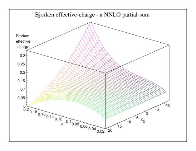
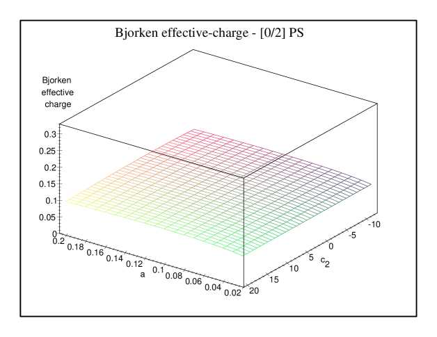
Fig. 4: Bjorken effective charge for $Q^{2}\,=\,20\,GeV^{2}$ plotted as a function of the renormalization scale and scheme, as parametrized by the coupling $x=\alpha_{s}(\mu^{2})/\pi$ and the second coefficient of the $\beta$ function: $c_{2}=\beta_{2}/\beta_{0}$. The upper plot shows the NNLO partial sum, while the lower plot shows the [0/2] Padé approximant.

5 Predicting the QCD $\beta$ function at 4 and 5 loops

Although no QCD observables have been calculated exactly beyond ${\cal O}(\alpha^{3})$, in fall of 1996 we had learned that a calculation of the 4-loop contribution to the QCD $\beta$ function was under way, and likely to be published soon. The prediction of the unknown 4-loop coefficient [EKSbeta] was therefore an important challenge and excellent testing ground for the new APAP method.

As a warm-up exercise one can test the APAP method on the 4-loop $\beta$ function of the $\Phi^{4}$ theory with $O(N)$ global vector symmetry [vkt], the latter being analogous to the $SU(N_{f})$ global symmetry of QCD. The results [EKSbeta] for $\beta_{3}$ in $O(N)$ $\Phi^{4}$ theory are shown in Figure 5. Clearly, the variant of APAP method denoted as $\langle A\rangle/n$ (see [EKSbeta] for details) is markedly superior to the naive PAP. The 5-loop $\beta$ function in this theory is also known [Chetyrkin5loop, Kleinert5Loop] and the corresponding APAP estimates also turn out to be very precise [EKSbeta]. Consequently this was the method of choice for the QCD 4-loop $\beta$ function.

Fig. 5: The 4-loop $\beta$-function coefficient $\beta_{3}$ in $\Phi^{4}$ theory with $O(N)$ symmetry. The exact results are denoted by black dots, joined by a solid line to guide the eye. Naive PAP results are denoted by diamonds, and APAP results obtained from the $\langle A\rangle/n$ type of correction are denoted by crosses. For comparison, also shown are APAP results obtained from the $\langle B\rangle/n^{2}$ type of correction, denoted by open circles.

The strategy for computing $\beta_{3}$, the 4-loop $\beta$ function coefficient, is as follows. We recall that $\beta_{3}$ is a cubic polynomial in the number of flavors $N_{f}$:

$$\beta_{3}=A_{3}+B_{3}N_{f}+C_{3}N_{f}^{2}+D_{3}N_{f}^{3},$$ (22)

where $D_{3}=1.49931$ (For $N_{C}=3$) is known from large-$N_{f}$ calculations [Gracey]. The known exact expressions for the 1-, 2- and 3-loop $\beta$ function are used as input to APAP, to predict the value of $\beta_{3}$ for a range of $N_{f}$ values. The predictions for $A_{3},B_{3},C_{3}$ are then obtained from fitting the APAP results for $0\leq N_{f}\leq 4$ to a polynomial of the form (22).

Shortly after the APAP prediction of $\beta_{3}$ [EKSbeta] the exact result was published in Ref. [beta4loop]. One important lesson from the exact results is that they contain qualitatively new color factors, corresponding to quartic Casimirs, analogous to light-by-light scattering diagrams in QED. Such terms are not present at 1-, 2- and 3-loop level, and therefore cannot be estimated using the Padé method. Numerically the correction due to these new color factors is not very large, but in principle the PAP estimates should be compared with the rest of the exact expression, as is done in the first three columns of Table I.

 $A_{3}$  23,600(900)  24,633  -4.20(3.70)    24,606  -0.11      $B_{3}$   -6,400(200) -6,375 -0.39(3.14) -6,374 -0.02   $C_{3}$ 350(70) 398.5 -12.2(17.6) 402.5 -1.00   $D_{3}$ input 1.499 - input