Towards a superformula for neutrinoless double beta decay

Abstract

A general Lorentz–invariant parameterization for the long-range part of the $0\nu\beta\beta$ decay rate is derived. Combined with the short range part this general parameterization in terms of effective $B-L$ violating couplings will allow it to extract the $0\nu\beta\beta$ limits on arbitrary lepton number violating theories. Several new nuclear matrix elements appear in the general formalism compared to the standard neutrino mass mechanism. Some of these new matrix elements have never been considered before and are calculated within pn-QRPA. Using these, limits on lepton number violating parameters are derived from experimental data on ⁷⁶Ge.

, , ,

1 Introduction

Double beta decay has been proven to be one of the most powerful tools to constrain $B-L$ violating physics beyond the standard model [1]. In recent years, besides the most restrictive limit on the effective neutrino Majorana mass [1, 2], stringent constraints on several theories beyond the Standard Model such as $R$–parity violating [3, 4, 5] as well as conserving [6] SUSY, leptoquarks [8], left–right symmetric models [9] and compositeness [10, 11] have been derived (for a review see [1]).

While the neutrino mass limit is based on the well-known mechanism exchanging a massive Majorana neutrino between two standard model $V-A$ vertices, the effective vertices appearing in the new contributions involve non–standard currents such as scalar, pseudoscalar and tensor currents.

Thus we felt motivated to consider the neutrinoless double beta decay rate in a general framework, parameterizing the new physics contributions in terms of all effective low-energy currents allowed by Lorentz-invariance. Such an ansatz allows one to separate the nuclear physics part of double beta decay from the underlying particle physics model, and derive limits on arbitrary lepton number violating theories. The first step of this work, treating the long–range part, is presented here. Although the general decay rate is independent of the underlying nuclear physics model, to extract quantitative limits values for nuclear matrix elements are needed. First limits are derived using matrix elements calculated in proton-neutron (pn) QRPA, partially already available in the literature and partially calculated here for the first time.

2 General Formalism

We consider the long–range part of neutrinoless double beta decay with two vertices, which are pointlike at the Fermi scale, and exchange of a light neutrino in between. The general Lagrangian can be written in terms of effective couplings $\epsilon^{\alpha}_{\beta}$, which correspond to the pointlike vertices at the Fermi scale so that Fierz rearrangement is applicable:

$${\cal L}=\frac{G_{F}}{\sqrt{2}}\{j_{V-A}^{\mu}J^{\dagger}_{V-A,\mu}+\sum_{\alpha,\beta}^{{}^{\prime}}\epsilon_{\alpha}^{\beta}j_{\beta}J^{\dagger}_{\alpha}\}$$ (1)

with the combinations of hadronic and leptonic Lorentz currents $J_{\alpha}^{\dagger}=\bar{u}{\cal O}_{\alpha}d$ respectively $j_{\beta}=\bar{e}{\cal O}_{\beta}\nu$ of defined helicity. The operators ${\cal O}_{\alpha,\beta}$ are defined as

$${\cal O}_{V-A}=\gamma^{\mu}(1-\gamma_{5})$$

$${\cal O}_{V+A}=\gamma^{\mu}(1+\gamma_{5})$$

$${\cal O}_{S-P}=(1-\gamma_{5})$$

$${\cal O}_{S+P}=(1+\gamma_{5})$$

$${\cal O}_{T_{L}}=\frac{i}{2}[\gamma_{\mu},\gamma_{\nu}](1-\gamma_{5})$$

$${\cal O}_{T_{R}}=\frac{i}{2}[\gamma_{\mu},\gamma_{\nu}](1+\gamma_{5}).$$ (2)

The prime indicates the sum runs over all contractions allowed by Lorentz–invariance, except for $\alpha=\beta=V-A$. Note that all currents have been scaled relative to the strength of the ordinary ($V-A$) interaction.

The effective Lagrangian given in eq. (1) represents the most general low-energy 4-fermion charged-current interaction allowed by Lorentz invariance. The interpretation of the effective couplings $\epsilon^{\alpha}_{\beta}$, however, depend on the specific particle physics model. Nevertheless one realizes the following general feature. Using only the SM fermion fields and working in the Majorana basis for the neutrinos ($\nu:=\nu_{L}+\nu_{L}^{C}$) it is easily seen that all currents involving operators proportional to ($1+\gamma_{5}$) violate lepton number by two units, i.e. the corresponding $\epsilon^{\alpha}_{\beta}$ must also be lepton-number violating. (Such LNV $\epsilon^{\alpha}_{\beta}$ are easily found, an example is given by R-parity violating supersymmetry treated in ref. [3, 4, 5].)

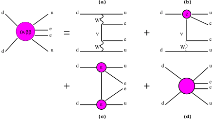
Figure 1: Feynman graphs of the general double beta rate: The contributions a) - c) correspond to the long range part, the contribution d) is the short range part (to be discussed elsewhere).

The double beta decay amplitude is proportional to the time-ordered product of two effective Lagrangians (see Fig. 1):

$$T({\cal L}_{(1)}{\cal L}_{(2)})=\frac{G_{F}^{2}}{2}T\{j_{V-A}J^{\dagger}_{V-A}j_{V-A}J^{\dagger}_{V-A}$$

$$+\epsilon_{\alpha}^{\beta}j_{\beta}J^{\dagger}_{\alpha}j_{V-A}J^{\dagger}_{V-A}+\epsilon_{\alpha}^{\beta}\epsilon_{\gamma}^{\delta}j_{\beta}J^{\dagger}_{\alpha}j_{\delta}J^{\dagger}_{\gamma}\}.$$ (3)

While the first term (contribution (a) in Fig. 1) corresponds to the standard model (SM) like neutrino exchange, and the 3rd term (contribution (c) in Fig. 1), which is quadratic in $\epsilon$ can be neglected, only the 2nd term (contribution (b)) is phenomenologically interesting. For this term one has to consider two general cases:

1) The leptonic SM $V-A$ current meets a left–handed non SM current $j_{\beta}$ with $\beta=S-P,T_{L}$. For this contribution the neutrino propagator is

$$\sim P_{L}\frac{q^{\mu}\gamma_{\mu}+m_{\nu}}{q_{\mu}q^{\mu}-m_{\nu}^{2}}P_{L}=\frac{m_{\nu}}{q_{\mu}q^{\mu}-m_{\nu}^{2}}$$ (4)

with the usual left– and right–handed projectors $P_{L/R}=\frac{1\mp\gamma_{5}}{2}$. This expression is proportional to the unknown neutrino Majorana mass $m_{\nu}\leq\sim 0.5eV$, for which no lower bound exists. Therefore no limits on the corresponding parameters $\epsilon_{\alpha}^{\beta}$ can be derived.

2) The leptonic SM $V-A$ current meets a right–handed non SM current $j_{\beta}$ with $\beta=S+P,V+A,T_{R}$. For this contribution the neutrino propagator is

$$\sim P_{L}\frac{q^{\mu}\gamma_{\mu}+m_{\nu}}{q_{\mu}q^{\mu}-m_{\nu}^{2}}P_{R}=\frac{q^{\mu}\gamma_{\mu}}{q_{\mu}q^{\mu}-m_{\nu}^{2}}$$ (5)

which is proportional to the neutrino momentum $q_{\mu}\simeq p_{F}\simeq 100MeV$ with the nuclear Fermi momentum $p_{F}$, and thus will produce stringent limits on corresponding $\epsilon_{\alpha}^{\beta}$.

Taking these considerations into account, we are left with three interesting contributions discussed in the following section. With the present half-life limit of the Heidelberg–Moscow experiment $T_{1/2}^{0\nu\beta\beta}>1.2\cdot 10^{25}y$ [1] and considering only one $\epsilon_{\alpha}^{\beta}$ at a time (evaluation ”on axis”)

$$[T_{1/2}^{0\nu\beta\beta}]^{-1}=(\epsilon_{\alpha}^{\beta})^{2}G_{0k}|ME|^{2}$$ (6)

where $G_{0k}$ denotes the phase space factors given in [12] and $|ME|$ the nuclear matrix elements discussed in the following. Note that evaluating ”on axis”, compared to the arbitrary evaluation, neglects interference terms of the different contributions. Although this is expected to be a small effect (see below), this remains to be discussed in the next step.

3 Calculational details and limits

3.1 SM meets $j_{V+A}J^{\dagger}_{V+A}$ and $j_{V+A}J^{\dagger}_{V-A}$

This contribution has been considered already in the context of left–right symmetric models [12, 15, 9]. For sake of completeness we repeat the updated results of [15] here in our notation: $\epsilon^{V+A}_{V+A}<7.9\cdot 10^{-7}$, $\epsilon^{V+A}_{V-A}<4.9\cdot 10^{-9}$ for the full calculation with arbitrary evaluation. Using s–wave approximation and ”on axis” evaluation as was done in this work the limits are reduced to $\epsilon^{V+A}_{V+A}<7.0\cdot 10^{-7}$, $\epsilon^{V+A}_{V-A}<4.4\cdot 10^{-9}$. This example confirms the expectation that these assumptions will only slightly (less than 10 %) affect the result.

It is worthwhile discussing the following subtlety in interpretation when comparing our ansatz and the work of [12]. Doi et al. [12] calculate the decay amplitude, writing down the Lagrangian of an explicitly left-right symmetric model. Therefore, their calculations do not only treat SM neutrinos, but contain also right-handed neutrinos. Nevertheless, the derivation of the decay amplitude for $0\nu\beta\beta$ decay is the same in both calculations, only some care is required when going from one notation to the other. For example, in the lepton-number violating $\langle\lambda\rangle$, defined in [12] as

$$\langle\lambda\rangle=\lambda\sum^{\prime}_{j}U_{ej}V_{ej}$$ (7)

where $\lambda\approx(m_{W_{L}}/m_{W_{R}})^{2}$, LNV is due to the product of mixing matrices $\sum^{\prime}_{j}U_{ej}V_{ej}$, which vanishes identically if LNV goes to zero. Thus, our (LNV) $\epsilon^{V+A}_{V+A}$ corresponds to $\langle\lambda\rangle$ of Doi et al. [12], (and not to $\lambda$). This example shows, that the use of only SM neutrinos in the derivation does not imply a loss of generality in our results, if the source of LNV of the particle physics model under consideration is carefully identified.

3.2 SM meets $j_{S+P}J^{\dagger}_{S+P}$ and $j_{S+P}J^{\dagger}_{S-P}$

Using s-wave approximation for the outgoing electrons and some assumptions according to [13, 4] one gets

$$ME_{S+P}^{S+P}=-ME_{S-P}^{S+P}=-\frac{F^{(3)}_{P}(0)}{Rm_{e}G_{A}}\Big{(}{\cal M}_{T^{{}^{\prime}}}+\frac{1}{3}{\cal M}_{GT^{{}^{\prime}}}\Big{)}.$$ (8)

The phase space factor is defined

$$G_{01}=\frac{(G_{F}G_{A})^{4}m_{e}^{4}}{{32}\pi^{5}(m_{e}R)^{2}ln2}\int F_{0}(Z,\epsilon_{1})p_{1}\epsilon_{1}F_{0}(Z,\epsilon_{2})p_{2}\epsilon_{2}$$

$$\delta(\epsilon_{1}+\epsilon_{2}+M_{f}-M_{i})d\epsilon_{1}d\epsilon_{2}$$ (9)

and the matrix elements (summation over nucleons $a,b$ is suppressed) are

$${\cal M}_{GT^{{}^{\prime}}} = \langle 0_{f}^{+}|h_{R}(\vec{\sigma_{a}}\vec{\sigma_{b}})\tau^{+}_{a}\tau^{+}_{b}|0_{i}^{+}\rangle$$ (10)

$${\cal M}_{T^{{}^{\prime}}} = \langle 0_{f}^{+}|h_{T^{{}^{\prime}}}\{(\vec{\sigma_{a}}\hat{\vec{r}}_{ab})(\vec{\sigma_{b}}\hat{\vec{r}}_{ab})$$ (11)

$$-\frac{1}{3}(\vec{\sigma}_{a}\vec{\sigma}_{b})\}\tau^{+}_{a}\tau^{+}_{b}|0_{i}^{+}\rangle.$$

$h_{R}$ and $h_{T^{{}^{\prime}}}$ are neutrino potentials defined as

$$h_{R} = \frac{2}{\pi}\frac{R^{2}}{m_{P}}\int_{0}^{\infty}dqq^{4}\frac{j_{0}(qr_{ab})f^{2}(q^{2})}{\omega(\omega+\overline{E})},$$ (12)

$$h_{T^{{}^{\prime}}} = \frac{2}{\pi}\frac{R^{2}}{m_{P}}\int_{0}^{\infty}dqq^{2}\frac{f^{2}(q^{2})}{\omega(\omega+\overline{E})}\{q^{2}j_{0}(qr_{ab})$$ (13)

$$-3\frac{q}{r_{ab}}j_{1}(qr_{ab})\}.$$

Here $R$ denotes the nuclear radius, $m_{P}$ the proton mass, $\epsilon_{i}$ and $p_{i}$ are electron energies and momenta, $F_{0}(Z,\epsilon_{i})$ and is the Fermi function. Further $\omega=\sqrt{q^{2}+m_{\nu}^{2}}$, $q=|\vec{q}|$, $\hat{r}=\vec{r}/r$ and $j_{k}(qr)$ are spherical Bessel functions. $(\omega+\overline{E})^{-1}$ is the energy denominator of the perturbation theory. The form factors $F^{a}_{i}(0)=F^{a}_{i}(q^{2})/f(q^{2})$ with $f(q^{2})=(1+q^{2}/m_{A}^{2})^{-2}$ ($m_{A}^{2}=0.85$ GeV) have been calculated in the MIT bag model in [14], $G_{A}\simeq 1.26$ and $G_{V}\simeq 1$.

Inserting the numerical value of the matrix elements ${\cal M}_{GT^{{}^{\prime}}}$ and ${\cal M}_{T^{{}^{\prime}}}$ (see [4] and Tab. 1), one derives $\epsilon^{S+P}_{S+P},\epsilon^{S+P}_{S-P}<1.1\cdot 10^{-8}$.

3.3 SM meets $j_{T_{R}}J^{\dagger}_{T_{R}}$ and $j_{T_{R}}J^{\dagger}_{T_{L}}$

In the tensor part the decay rate depends on the phase space $G_{01}$ and new matrix elements not considered in the literature.

For the hadronic $T_{R}$ contribution one gets under the assumptions used above

$$ME^{T_{R}}_{T_{R}}=-\alpha_{1}\frac{2}{3}{\cal M}_{GT^{{}^{\prime}}}+\alpha_{1}{\cal M}_{T^{{}^{\prime}}}$$ (14)

with

$$\alpha_{1} = \frac{4T_{1}^{(3)}(0)G_{V}(1-2m_{P}(G_{W}/G_{V}))}{G_{A}^{2}Rm_{e}}.$$ (15)

Again $T_{1}^{(3)}(0)$ has been taken from [14] and the strength of the induced weak magnetism $(G_{W}/G_{V})=\frac{\mu_{P}-\mu_{n}}{2m_{P}}\simeq\frac{-3.7}{2m_{P}}$ is obtained by the CVC hypothesis. The involved nuclear matrix elements have been calculated in the QRPA–approach of [15, 16]. Inserting the values obtained for the special case of ⁷⁶Ge (see Tab. 1) yields $\epsilon^{T_{R}}_{T_{R}}<1.7\cdot 10^{-9}$.

For the hadronic $T_{L}$ contribution in leading order of $(1/m_{P})$ one finds

$$ME^{T_{R}}_{T_{L}}=\alpha_{2}{\cal M}_{F^{{}^{\prime}}}-\alpha_{3}\Big{(}{\cal M}_{T^{{}^{\prime\prime}}}+\frac{1}{3}{\cal M}_{GT^{{}^{\prime\prime}}}\Big{)}$$ (16)

with

$${\cal M}_{F^{{}^{\prime}}} = \langle 0_{f}^{+}|h_{R}\tau_{a}^{+}\tau_{b}^{+}|0_{i}^{+}\rangle$$ (17)

$${\cal M}_{GT^{{}^{\prime\prime}}} = \langle 0_{f}^{+}|h_{R\omega}(\vec{\sigma_{a}}\vec{\sigma_{b}})\tau^{+}_{a}\tau^{+}_{b}|0_{i}^{+}\rangle$$ (18)

$${\cal M}_{T^{{}^{\prime\prime}}} = \langle 0_{f}^{+}|\omega h_{T^{{}^{\prime\prime}}}\{(\vec{\sigma_{a}}\hat{\vec{r}}_{ab})(\vec{\sigma_{b}}\hat{\vec{r}}_{ab})$$ (19)

$$-\frac{1}{3}(\vec{\sigma}_{a}\vec{\sigma}_{b})\}\tau^{+}_{a}\tau^{+}_{b}|0_{i}^{+}\rangle.$$

The neutrino potentials are

$$h_{R}\omega = \frac{2}{\pi}\frac{R^{3}}{m_{P}}\int_{0}^{\infty}dqq^{4}\frac{j_{0}(qr_{ab})f^{2}(q^{2})}{(\omega+\overline{E})},$$ (20)

$$h_{T^{{}^{\prime\prime}}} = \frac{2}{\pi}\frac{R^{3}}{m_{P}}\int_{0}^{\infty}dqq^{2}\frac{f^{2}(q^{2})}{(\omega+\overline{E})}\{q^{2}j_{0}(qr_{ab})$$ (21)

$$-3\frac{q}{r_{ab}}j_{1}(qr_{ab})\}.$$

and

$$\alpha_{2} = \frac{4(2{\hat{T}}_{2}^{(3)}(0)-T_{1}^{(3)}(0))G_{V}}{G_{A}^{2}Rm_{e}},$$ (22)

$$\alpha_{3} = \frac{4T_{1}^{(3)}(0)(G_{P}/G_{A})}{G_{A}R^{2}m_{e}}.$$ (23)

Here $\hat{T}_{2}^{(3)}(0)$ has been taken from [14]$,G_{P}/G_{A}=2m_{P}/m_{\pi}^{2}$ and $\omega$ is the neutrino energy. Again the matrix elements have been calculated in the model of [15, 16]. A limit of $\epsilon^{T_{R}}_{T_{L}}<7.3\cdot 10^{-10}$ has been obtained. Factors $R$ have been arbitrarily absorbed into the definition ${\cal M}_{GT^{{}^{\prime\prime}}}$ and ${\cal M}_{T^{{}^{\prime\prime}}}$ to get dimensionless quantities. One should notice that the corresponding factor included in $\alpha_{3}$ compensates this choice.

4 Conclusion

We have presented a general parameterization for the long range part of the neutrinoless double beta decay rate in terms of effective couplings. The resulting bounds are summarized in Tab. 2. Combined with the short range part and contributions of derivative couplings, this parameterization will give the double beta decay constraints for arbitrary lepton number violating theories beyond the SM. The next step should include these contributions and discuss interference terms.

${\cal M}_{GT^{{}^{\prime}}}$	2.95
${\cal M}_{F^{{}^{\prime}}}$	-0.663
${\cal M}_{GT^{{}^{\prime\prime}}}$	8.78
${\cal M}_{T^{{}^{\prime}}}$	0.224
${\cal M}_{T^{{}^{\prime\prime}}}$	1.33

Table 1: Relevant Nuclear Matrix Elements calculated in pn-QRPA

$\epsilon^{V+A}_{V-A}$	$4.4\cdot 10^{-9}$
$\epsilon^{V+A}_{V+A}$	$7.0\cdot 10^{-7}$
$\epsilon^{S+P}_{S-P}$	$1.1\cdot 10^{-8}$
$\epsilon^{S+P}_{S+P}$	$1.1\cdot 10^{-8}$
$\epsilon^{TR}_{TL}$	$6.4\cdot 10^{-10}$
$\epsilon^{TR}_{TR}$	$1.7\cdot 10^{-9}$

Table 2: Limits on effective $B-L$ violating couplings evaluated “on axis”

References

• [1] H.V. Klapdor–Kleingrothaus, in [7]
• [2] L. Baudis et al. (Heidelberg–Moscow collab.), Phys. Lett. B 407 (1997) 219
• [3] M. Hirsch, H.V. Klapdor–Kleingrothaus, S.G. Kovalenko, Phys. Rev. Lett. 75 (1995) 17, M. Hirsch, H.V. Klapdor–Kleingrothaus, S. Kovalenko, Phys. Rev. D 53 (1996) 1329
• [4] M. Hirsch, H.V. Klapdor–Kleingrothaus, S.G. Kovalenko, Phys. Lett. B 372 (1996) 181, Erratum: Phys. Lett. B 381 (1996) 488
• [5] H. Päs, M. Hirsch, H.V. Klapdor–Kleingrothaus, in preparation
• [6] M. Hirsch, H.V. Klapdor–Kleingrothaus, S.G. Kovalenko, Phys. Lett. B 398 (1997) 311; Phys. Rev. D 57 (1998) 1947; contribution in [7]
• [7] H.V. Klapdor–Kleingrothaus, H. Päs (Eds.), Proc. Int. Conf. “Beyond the Desert - Accelerator- and Non-Accelerator Approaches”, Castle Ringberg, Germany, 1997
• [8] M. Hirsch, H.V. Klapdor–Kleingrothaus, S.G. Kovalenko, Phys. Lett. B 378 (1996) 17 and Phys. Rev. D 54 (1996) R4207
• [9] M. Hirsch, H.V. Klapdor–Kleingrothaus, O. Panella, Phys. Lett. B 374 (1996) 7
• [10] O. Panella, in [7]
• [11] E. Takasugi, in [7]
• [12] M. Doi, T. Kotani, E. Takasugi, Progr. Theor. Phys. Suppl. 83 (1985) 1
• [13] T. Tomoda, Rep. Progr. Phys. 54 (1991) 53
• [14] S. Adler et al., Phys. Rev. D 11, (1975) 3309
• [15] K. Muto, E. Bender, H.V. Klapdor, Z. Phys. A 334 (1989) 177,187;
• [16] A. Staudt, K.Muto, H.V. Klapdor–Kleingrothaus, Europhys. Lett. 13 (1990) 31; M. Hirsch, K.Muto, T.Oda, H.V. Klapdor–Kleingrothaus, Z. Phys. A 347 (1994) 151
Refer to caption