[]

The Plasmon Damping Rate for $T\rightarrow T_{C}$

Abstract

The plasmon damping rate in scalar field theory is computed close to the critical temperature. It is shown that the divergent result obtained in perturbation theory is a consequence of neglecting the thermal renormalization of the coupling. Taking this effect into account, a vanishing damping rate is obtained, leading to the critical slowing down of the equilibration process.

The behaviour of field theory at finite temperature has been the subject of intense study in the recent past, mainly in connection with the investigation of phase transitions in the early universe and of the properties of the quark-gluon plasma. Most of the effort has been devoted to the calculation of time-independent quantities, like the QCD pressure or the electroweak effective potential. Thus, finite temperature field theory in thermal equilibrium has been mainly employed in this kind of studies.

More recently, time-dependent processes have been taken in consideration, like the generation of the cosmological baryon asymmetry or the dynamics of scalar fields in inflationary models.

An example of a dynamical quantity which has received much attention in the recent literature is the plasmon damping rate, defined as

$$\gamma(T)\equiv\frac{\Pi_{I}(m(T),0)}{2m(T)}\;,$$ (1)

where $m(T)$ is the thermal mass and $\Pi_{I}$ is the imaginary part of the two-point retarded green function.

$\gamma(T)$ gives the inverse relaxation time of space independent fluctuations at the temperature $T$ [1], and in $\lambda\Phi^{4}/4!$ theory it emerges at two-loops in perturbation theory. In refs. [2, 3] it was computed as

$$\gamma_{p.t.}=\frac{1}{1536\pi}\,l_{qu}\,\lambda^{2}T^{2}\,$$ (2)

where $l_{qu}=1/m(T)=\left(\frac{\lambda T^{2}}{24}\right)^{-1/2}$ is the Compton wavelength, and the temperature $T$ is much larger than any mass scale of the $T=0$ theory.

In refs. [4] it was shown that the above two-loop result can be reproduced in the classical theory provided that the Compton wavelength $l_{qu}$ is identified with the classical correlation length $l_{c}$. The above result can be understood realizing that $\gamma$ probes the theory at scales $\omega=m(T)\ll T$ (if $\lambda$ is perturbatively small), where the Bose-Einstein distribution function is approximated by its classical limit,

$$N(\omega)=\frac{1}{e^{\beta\omega}-1}\rightarrow\frac{1}{\beta m(T)}\;\;\;\;\;\;\;\;\,\;\;({\rm if}\;\beta\omega\ll 1)\;,$$ (3)

with $\beta=1/T$. Considering for instance the 1-1 component of the propagator in the real-time formalism,

$$\Delta_{11}={\cal P}\frac{1}{k^{2}-m^{2}}-2\pi i\delta(k^{2}-m^{2})\left(\frac{1}{2}+N(|k_{0}|)\right),$$ (4)

we see that when the loop momenta are $k_{0}\ll T$ the ‘statistical’ part of the imaginary part of the propagator dominates over the ‘quantum’ part, i.e. $N\gg 1/2$, and the leading order result can be obtained neglecting the $T=0$ quantum contributions to the loop corrections.

The above argument has been employed to motivate the use of classical equations of motion in the study of the evolution of long wavelength modes in scalar and gauge theories. More recently, this approach has been improved by many authors including the effect of Hard Thermal Loops in the equations of motion for the ‘soft’ modes (see for instance [5, 6]). The separation between hard and soft modes has been made explicit in ref. [6] by introducing a cutoff $\Lambda$ such that $m(T)\mathrel{\vbox{\hbox{$<$}\nointerlineskip\hbox{$\sim$}}}\Lambda<T$.

In this letter we want to investigate further the relation between thermal and classical field theory, extending the computation of the damping rate to temperatures close to the critical one. The 1-loop thermal mass is now given by $m^{2}(T)=-\mu^{2}+\lambda T^{2}/24$. In the limit

$\displaystyle T\rightarrow T_{C}=\sqrt{\frac{24\mu^{2}}{\lambda}}$

the thermal mass vanishes and the behaviour of the infrared (IR) modes is exactly statistical, see eq. (3).

The divergence of the correlation length at the critical point implies that the two-loop/classical expression in eq. (2) diverges as well. Physically, this would mean that the lifetime of long wavelength fluctuations is getting shorter and shorter as the critical temperature is approached, a behaviour opposite to the critical slowing down exhibited by condensed matter systems and reproduced in the theory of dynamic critical phenomena [7].

The failure of (resummed) perturbation theory close to the critical point is by no means unexpected. When $T\simeq T_{C}$ the effective expansion parameter, ${\it i.e.}\;\lambda T/m(T)$, diverges, and it is well known that the – super-daisy resummed – effective potential is not even able to reproduce the second order phase transition of the real scalar theory [8, 9].

In refs.[10, 11, 12] it was shown that the key effect which is missed by perturbation theory is the dramatic thermal renormalization of the coupling constant, which vanishes in the critical region. This can be understood in the framework of the Wilson Renormalization Group. The IR regime of the four-dimensional field theory at $T=T_{C}$ is related to that of the three-dimensional theory at $T=0$. In particular, the three-dimensional running coupling is obtained from the four-dimensional one by [11]

$\displaystyle\lambda_{3D}(\Lambda)=\lambda(\Lambda)\frac{T}{\Lambda}\,.$

At the critical point, $\lambda_{3D}$ flows in the IR to the Wilson-Fischer fixed point value $\lambda^{*}_{3D}\neq 0$, so that the four-dimensional coupling vanishes,

$\displaystyle\lambda(\Lambda)\rightarrow\frac{\Lambda}{T}\lambda^{*}_{3D}\;\;\;({\rm for}\;T\simeq T_{C}\;{\rm and}\;\Lambda\rightarrow 0)\,.$

The critical exponent governing the vanishing of $\lambda$ is the same as that for $m(T)$, so that the ratio $\lambda(T)T/m(T)$ goes to a finite value at $T_{C}$, and a second order phase transition is correctly reproduced.

We will show that the running of the coupling constant for $T\simeq T_{C}$ is crucial also in reproducing the expected critical slowing down, i.e. the vanishing of the plasmon damping rate. As a first rough ansatz one could just replace the tree coupling $\lambda$ with the thermally renormalized one in eq. (3) and readily obtain the expected behaviour. As we will see, this gives a wrong answer, due to the logarithmic singularity of the on-shell imaginary part when $m(T)$ vanishes.

In the rest of the letter we will illustrate the computation of the plasmon damping rate in the framework of the Wilson renormalization group approach for thermal modes (TRG) introduced in ref. [12]. This method allows a computation of the damping rate for any value of $T$, from very high values, where perturbation theory works, to the critical region, where renormalization group methods like those of [7] are necessary to resum infrared divergencies. But the TRG is applicable also in the intermediate region, in which none of these methods can be applied.

For a detailed discussion of the formulation of the RG in the real-time formalism of high temperature field theory the reader is referred to refs. [12, 13]. The basic idea is to introduce a momentum cut-off in the thermal sector by modifying the Bose-Einstein distribution function appearing in the tree-level propagator as

$$N(k_{0})\rightarrow N_{\Lambda}(k_{0})=N(k_{0})\theta(|\vec{k}|-\Lambda)\;,$$ (5)

where $\theta(x)$ is Heavyside’s step function, but smooth functions can be used as well. Following Polchinski [14], the effective action and the green functions can then be defined non-perturbatively by means of evolution equations in $\Lambda$. For $\Lambda\gg T$ the statistical part of the propagators is exponentially damped by the Bose-Einstein distribution function, and we have the $T=0$ renormalized quantum field theory (with all the $T=0$ quantum fluctuations included). As $\Lambda$ is lowered, thermal fluctuations with $|\vec{k}|>\Lambda$ are integrated out. In the limit $\Lambda\rightarrow 0$ the full thermal field theory in equilibrium is recovered.

We will compute the real and imaginary parts of the (1-1) component of the self-energy

$$\Sigma_{11}(\omega\pm i\varepsilon,\vec{k};\Lambda)=\Sigma^{R}_{11}(\omega,\vec{k};\Lambda)\pm i\Sigma^{I}_{11}(\omega,\vec{k};\Lambda)$$ (6)

where the real part is the same as that of the self-energy appearing in the propagator, $\Sigma^{R}_{11}(k;\Lambda)=\Pi_{R}(k;\Lambda)$ and the imaginary part is linked to $\Pi_{I}$ in (1) by $\Pi_{I}=\Sigma^{I}_{11}/(1+2N)$ [15].

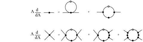
FIG. 1.: Schematic representation of the evolution equations for the two–and four– point functions.

The evolution equation for $\Sigma_{11}(\Lambda)$ is represented schematically in the upper line of Fig.1. The full dots indicate full, $\Lambda$-dependent vertices and propagators, which contain all the thermal modes with $|\vec{k}|>\Lambda$. The empty dot represents the kernel of the evolution equation, which substitutes the full propagator in the corresponding leg. Its (1-1) component is given by

$\displaystyle K_{\Lambda,11}(k)=-\rho_{\Lambda}(k)\varepsilon(k_{0})\Lambda\delta(|\vec{k}|-\Lambda)N(|k_{0}|)\,$

where $\rho_{\Lambda}(k)$ is the full spectral function and $\varepsilon(x)=\theta(x)-\theta(-x)$.

In order to determine the $\Lambda$-dependent four-point function we must consider the system containing also the second equation in Fig.1. Since the theory has a – possibly spontaneously broken – $Z_{2}$ symmetry, the trilinear couplings are not arbitrary and will be determined from the mass and the quartic coupling as we will indicate below. All n-point vertices with n$>$4 will be neglected.

The initial conditions for the evolution equations are given at a scale $\Lambda=\Lambda_{0}\gg T$ (due to the exponential damping in the Bose-Einstein function, $\Lambda\mathrel{\vbox{\hbox{$>$}\nointerlineskip\hbox{$\sim$}}}10\,T$ will be enough). Here, the effective action of the theory is approximated by

$\displaystyle\Gamma_{\Lambda_{0}}(\Phi)=\int d^{4}x\left[\frac{1}{2}(\partial\Phi)^{2}-\frac{1}{2}\mu^{2}_{\Lambda_{0}}\Phi^{2}-\frac{\lambda_{\Lambda_{0}}}{4!}\Phi^{4}\right]\;,$

where $\mu^{2}_{\Lambda_{0}}$ and $\lambda_{\Lambda_{0}}$ are the renormalized parameters of the $T=0$ theory. We are interested to the case in which the $Z_{2}$-symmetry is broken at $T=0$, so we will take $\mu^{2}_{\Lambda_{0}}<0$.

Then, we make the following approximations to the full propagator and vertices appearing on the RHS of the evolution equations:
${\it i)}$ the self-energy in the propagator is approximated by a running mass, $\Pi(k;\Lambda)\simeq m_{\Lambda}^{2}$ given by

$\displaystyle m_{L}^{2}=\mu^{2}_{\Lambda}\;\,({\rm if}\;\mu^{2}_{\Lambda}>0)\;,\;\;\;\;-2\mu^{2}_{\Lambda}\;\,({\rm if}\;\mu^{2}_{\Lambda}<0)$

${\it ii)}$ the four-point function is approximated as

$\displaystyle\Gamma^{(4)}_{\Lambda}(p_{i})\simeq-\lambda_{\Lambda}-i\eta_{\Lambda}(p_{i})\;,$

${\it iii)}$ the three-point function is given by

$\displaystyle\Gamma^{(3)}_{\Lambda}(p_{i})\simeq 0\;\,({\rm if}\;\mu^{2}_{\Lambda}>0)\;,\;\;\;\;\sqrt{-6\lambda_{\Lambda}\mu^{2}_{\Lambda}}\;\,({\rm if}\;\mu^{2}_{\Lambda}<0)\,.$

Moreover, all vertices with at least one of the thermal indices different from 1 will be neglected.

Some comments are in order at this point. In perturbation theory, the on-shell imaginary part is given by the two-loop setting sun diagram. The evolution equations of Fig.1 contain instead only one-loop integrals, so how can an imaginary part emerge? The crucial point here is that the momentum dependence of the imaginary part of the four-point function has to be taken into account (see point $ii)$). When the latter is inserted into the upper equation, $\Pi_{I}$ is generated.

As long as the $\Lambda$-dependent action is in the broken phase, trilinear couplings will be present. By neglecting the imaginary part of the self-energy in the propagators on the RHS (point i) above), we loose the contribution to $\Pi_{I}$ obtained by cutting the second diagram in the RHS of the upper equation of Fig.1. However, if we restrict ourselves to temperatures $T\geq T_{C}$, the trilinear couplings will be different form zero only in a limited range of $\Lambda$. They will not contribute in the IR, where the dominant contributions to the on-shell imaginary part emerge (see Fig. 3). The error induced by this approximation can be estimated noticing that the contribution we are neglecting is of the same nature as the one obtained by inserting the last diagram of the second equation in the equation for the two-point function. The latter is taken into account and its effect on the full imaginary part is of the order of a few percent.

We have now a system of four evolution equations for $\Pi_{R}(k;\Lambda)\simeq m_{\Lambda}^{2}$, $\Pi_{I}(k;\Lambda)$, $\lambda_{\Lambda}$, and $\eta_{\Lambda}(p_{i})$, with initial conditions $m_{\Lambda_{0}}^{2}=-2\mu_{\Lambda_{0}}^{2}$, $\lambda_{\Lambda_{0}}$, and $\Pi_{I}(k;\Lambda_{0})=\eta_{\Lambda_{0}}(p_{i})=0$, respectively. Moreover, the subsystem for $m_{\Lambda}^{2}$ and $\lambda_{\Lambda}$ is closed and can be integrated separately. So we proceed as follows. Fixing the temperature, we first integrate the subsystem for $m_{\Lambda}^{2}$ and $\lambda_{\Lambda}$ down to $\Lambda=0$ in order to find the plasmon mass, $m^{2}_{\Lambda=0}$. Then we fix the external momentum of $\Pi_{I}$ on this mass-shell, $k=(m^{2}_{\Lambda=0},\vec{0})$ and integrate the full system from $\Lambda=\Lambda_{0}$ down to $\Lambda=0$.

In Fig.2 we plot the results for the damping rate $\gamma$ and the coupling constant at $\Lambda=0$, as a function of the temperature. The dashed line has been obtained by keeping the coupling constant fixed ($\Lambda$-independent) to its $T=0$ value ($\lambda=10^{-2}$), and reproduces the divergent behaviour found in perturbation theory (eq. (2)). The crucial effect of the running of the coupling constant is seen in the behaviour of the dot-dashed line, which represents the main result of this letter. For temperatures close enough to $T_{C}$, the coupling constant (solid line in Fig.2) is dramatically renormalized and it decreases as

$\displaystyle\lambda_{\Lambda=0}(T)\sim t^{\nu}$

where $t\equiv(T-T_{C})/T_{C}$ and we find $\nu\simeq 0.53$. The mass also vanishes with the same critical index. The decreasing of $\lambda$ drives $\gamma$ to zero, but with a different scaling law,

$\displaystyle\gamma_{\Lambda=0}(T)\sim t^{\nu}\log t\;.$

The above expression can be understood noticing that the two-loop contribution to $\Pi_{I}$, computed at vanishing $\omega=m(T)$, goes as $\lambda^{2}\log m(T)$. The RG result replaces $\lambda$ with the renormalized coupling, then from (1) we have

$\displaystyle\gamma\sim\frac{\lambda_{\Lambda=0}^{2}}{m_{\Lambda=0}}\log m_{\Lambda=0}\sim t^{\nu}\log t\;.$

FIG. 2.: Temperature dependence of the coupling constant (solid line), and of the damping rate with the effect of the running of $\lambda$ included (dash-dotted) and excluded (dashed). The values for $\gamma$ have been multiplied by a factor of $10$.

Taking couplings bigger than the one used in this letter ($\lambda=10^{-2}$), the deviation from the perturbative regime starts to be effective farther from $T_{C}$. Defining an effective temperature as $\lambda_{\Lambda=0}(T)/\lambda_{\Lambda_{0}}\leq 1/2$ for $T_{C}<T\leq T_{e}ff$ we find that $t_{eff}$ scales roughly as $t_{eff}\sim\lambda_{\Lambda_{0}}$.

In Fig.3 we plot the running of $\lambda_{\Lambda}(T)$ and $\gamma_{\Lambda}(T)$ for two different values of the temperature. When $T\gg T_{C}$ most of the running takes place for $\Lambda\mathrel{\vbox{\hbox{$>$}\nointerlineskip\hbox{$\sim$}}}\Lambda_{soft}$, so it is safe to stop the running at this scale neglecting the effect of soft loops. When $T\rightarrow T_{C}$ this is not possible any longer, since most of the running of $\lambda$ and $\gamma$ takes place for $\Lambda\mathrel{\vbox{\hbox{$<$}\nointerlineskip\hbox{$\sim$}}}\Lambda_{soft}$. Thus, the vanishing of the mass gap forces us to take soft thermal momenta into account.

FIG. 3.: $\Lambda$-running of the coupling constant $\lambda$ and of the damping rate $\gamma$ for two different values of $t=(T-T_{C})/T_{C}$. The values of $\gamma$ (dot-dashed lines) have been multiplied by 500.

In conclusion, we have obtained the critical slowing down of long wavelength fluctuations in the framework of high temperature relativistic quantum field theory. The dominant effect has been shown to be the thermal renormalization of the coupling constant, which turns the divergent behaviour of the plasmon damping rate into a vanishing one. The notion of quasiparticle turns out to be valid much closer to the critical regime than the perturbative result would indicate. Indeed, for $\lambda=10^{-2}$, the ratio $\gamma/m(T)$ becomes larger than unity for $t\mathrel{\vbox{\hbox{$<$}\nointerlineskip\hbox{$\sim$}}}10^{-5}$ in perturbation theory, whereas the RG result is still $\gamma/m(T)\simeq 0.3$ at $t\simeq 10^{-9}$.

In a cosmological setting, the increasing lifetime of the fluctuations of the order parameter may modify the dynamics of second order – or weakly first order – phase transitions. Indeed, if the thermalization rate of long wavelength fluctuations exceeds the expansion rate of the Universe, the phase transition will take place out of thermal equilibrium [16]. This would lead to a scenario for the formation of topological defects similar to that discussed by Zurek in [17].

Acknowledgments
It is a pleasure to thank M. D’Attanasio – with whom this work was initiated – D.Comelli, and A. Riotto for inspiring discussions.

REFERENCES

- [1] A. Weldon, Phys. Rev. D28 (1983) 2007.
- [2] R.R. Parwani, Phys. Rev D45 (1992) 4695; ibid. D48 (1993) 5965 (E).
- [3] E. Wang and U. Heinz, Phys. Rev. D53 (1996) 899
- [4] G. Aarts and J. Smit, Pys. Lett. B393 (1997) 395; Nucl. Phys. B511 (1998) 451; W. Buchmüller and A. Jacovác, Phys. Lett. B407 (1997) 39.
- [5] M. Gleiser and R.O. Ramos, PRD50 (1994), 2441; C. Greiner and B. Müller, Phys. Rev. D55 (1997) 1026; P.Arnold, D. Son, and L. Yaffe, Phys. Rev. D55 (1997) 6264; E. Iancu, hep-ph/9710543; D. Bödeker, hep-ph/9801430.
- [6] W. Buchmüller and A. Jacovác, hep-th /9712093.
- [7] P.C. Hohenberg and B.I Halperin, Rev. Mod. Phys. 49 (1977) 435.
- [8] J.R. Espinosa, M. Quiros and F. Zwirner, Phys. Lett. B291 (1992) 115.
- [9] W. Buchmüller, Z. Fodor, T. Helbig and D. Walliser, Ann. Phys. 234 (1994) 260.
- [10] P.Elmfors, Z. Phys. C56 (1992) 601.
- [11] N. Tetradis and C. Wetterich, Nucl. Phys. B398 (1993) 659.
- [12] M. D’Attanasio and M. Pietroni, Nucl. Phys. B472 (1996) 711.
- [13] M. D’Attanasio and M. Pietroni, Nucl. Phys. B498 (1997) 443.
- [14] J. Polchinski, Nucl. Phys. B231 (1984) 269.
- [15] N.P. Landsman and Ch.G. van Weert, Phys. Rep. 145 (1987) 141.
- [16] P.Elmfors, K.Enqvist and I.Vilja Nucl. Phys. B422 (1994) 1994; Nucl.Phys. B412 (1994) 459.
- [17] W.H. Zurek Phys. Rep. 276 (1996) 177.