MZ-TH/98-16
First Results with a new Method for calculating 2-loop Box-Functions

Abstract

We describe a first attempt to calculate scalar 2-loop box-functions with arbitrary internal masses, applying a novel method proposed in [1]. Four of the eight integrals are accessible to integration by means of the residue theorem, leaving a rational function in the remaining variables. The result of the procedure is a three- or sometimes two-dimensional integral representation over a finite volume that can be further evaluated using numerical methods.

The study of higher-loop quantum corrections in QFTs is accompanied by rapidly increasing computational challenges. While in pure QED e.g. the presence of only one mass scale allows relative high loop orders to be evaluated [2], the feasibility of loop calculations in the general case with arbitrary internal masses has up to now been cut off at the two-loop level.

In recent years much work has been done on two-loop integrals with arbitrary internal masses of the self-energy- and vertex-type. These functions could be reduced to double integrals with manageable numerical behaviour [3, 4, 5, 6] (c.f. [7, 8] for another approach at these diagrams). Not much seems to be known, however, about the different two-loop corrections to scattering-amplitudes (Fig. 1) involving arbitrary-mass propagators which will become of some importance for probing new physics in $W^{+}W^{-}$-processes or in a Muon-collider, for example. Some of these topologies factorize into products of one-loop functions, i.e. no propagator shares both loop-momenta. Others are one-loop functions containing other one-loop functions as subtopologies (Fig. 1, third column). Rather than analyzing all of these functions, we focus our attention on five four-point topologies. They are all obtained by shrinking propagators in the two basic four-point topologies and . Two of them are of crossed type where two propagators share both loop-momenta (first column) and three of planar type (second column). There is no striking difference to the graphs in the third column. For example the first graph in the first row, third column relates to the graph in the second row, second column if we shrink the appropriate propagator.

The importance of the four point function derives not only from the fact that it describes the first scattering amplitude (2 $\rightarrow$ 2), but also from the fact that the multiparticle scattering amplitudes, involving $n$-point functions, $n\geq 5$, are closely related to the four point functions [9].

We will see below how this relation emerges in our method at the two-loop level.

The idea behind our method is to perform four of the integrals with Cauchy’s residue theorem and evaluate at least one of the remaining ones analytically, leaving a two- or three-dimensional representation for numerical evaluation.

This article is organized as follows: In the first two sections we describe how one can generally perform four integrations with the residue theorem alone and analyze the structure of the result. In the remaining sections we will complete the calculation for a graph of type in a special kinematic case, always keeping in mind the more general graphs, notably and as we go along. In section 4 we look at some of the results and discuss what possible problems we need to be concerned with in some limiting kinematical regimes.

Figure 1: Possible 2-loop box-topologies. Starting from class I, where all topologies are constructed by appending 4 external legs to the 2-loop master-topology, one can construct all other box-topologies by successive cancellation of internal propagators.

1 Integrating the middle variables

The functions under consideration can generally be written as

$$V=\int d^{4}k\int d^{4}l\,\frac{1}{P_{l,m_{1}}\,P_{l+k,m_{2}}\,P_{k,m_{3}}\cdots},$$ (1)

with five to seven inverse scalar propagators of the form $P_{l,m_{i}}=(l+p)^{2}-m_{i}^{2}+i\eta$, $l$ denoting a loop-momentum and $p$ some combination of external 4-momenta. Note that we do not attach an index $i$ to the $\eta$ from the Feynman prescription since we will choose them all to be equal. $V$ depends on six independent kinematic variables, a possible choice being the Mandelstam-variables $s$, $t$ and $u$ together with the masses $m_{i}$ of the four external particles and the condition $s+t+u=\sum_{i}m_{i}^{2}$. We will, however, need to choose an explicit Lorentz frame for our purposes.

When trying to perform one of the integrals using the residue theorem, it is very attractive to first linearize all the propagators $P_{i}$ with respect to the corresponding variable since this makes the detection of poles particularly simple and does not introduce unnecessary square roots inhibiting further integrations. Due to the signature of the Minkowski metric this linearization can easily be done in one pair of variables. Choosing $l_{1}$ and $k_{1}$ for linearization and applying the shift

$$l_{0}\longrightarrow l_{0}+l_{1},\qquad k_{0}\longrightarrow k_{0}+k_{1},$$ (2)

a propagator $P_{l}$ undergoes the transformation

$$(l+p)^{2}-m^{2}+i\eta=(l_{0}+p_{0})^{2}-(l_{1}+p_{1})^{2}-(l_{2}+p_{2})^{2}-(l_{3}+p_{3})^{2}-m^{2}+i\eta\,$$

$$\longrightarrow(l_{0}+p_{0})^{2}+2\,l_{1}\,(l_{0}+p_{0}-p_{1})-p_{1}^{2}-(l_{2}+p_{2})^{2}-(l_{3}+p_{3})^{2}-m^{2}+i\eta.$$ (3)

This shift can safely be done since the functions defined by topologies I a), II a), and I b) - III b) converge absolutely as can be seen by counting powers.

Closing the contour in the upper half-plane and using the residue theorem to carry out the $l_{1}$- and $k_{1}$-integrations, one obtains constraints for the $l_{0}$- and $k_{0}$-integrations. This appearance of constraints is due to the position of poles in the complex $l_{1}$- and $k_{1}$-planes either in the upper or the lower half and hence either contributing as a residue or not. These constraints affect the $l_{0}$- and $k_{0}$-integrations only because no other loop-variables appear in the $l_{1}$-linear term in (1). We will return to these constraints in the next section.

Noticing that the integrations over the variables $l_{2}$, $l_{3}$, $k_{2}$ and $k_{3}$ are still unbounded, suggests solving two of them with the residue theorem again. In [1] it was shown how the linearization necessary for simplifying this task can be carried out in what we may call the middle variables: $k_{1}$, $l_{1}$, $k_{2}$ and $l_{2}$. We will briefly repeat the argument.

As a consequence of conservation of four-momentum, the external legs of any four-point function span a 3-dimensional subspace of momentum-space—the so-called parallel space. Using Lorentz-invariance, its complement—the orthogonal space—can always be chosen to be parallel to the 3-axis. The 3-components of the loop-momenta do not mix with any external momenta then:

$$P_{l} = l_{3}^{2}+(\textit{something real})+i\eta,$$

$$P_{l+k} = (l_{3}+k_{3})^{2}+(\textit{something real})+i\eta,$$

$$P_{k} = k_{3}^{2}+(\textit{something real})+i\eta.$$

Hence the poles of the integrand in the complex $l_{3}$, $k_{3}$ and $(l_{3}+k_{3})$-planes respectively are all located in the first and third quadrant.

At this stage one can make contact to the case of a general $n$-point function. For $n\geq 5$ the 3-components do mix with external momenta. But the very fact that $n\geq 5$ ensures that after undertaking appropriate partial fraction in the propagators the convergence of all integrals is sufficiently strong so that termwise linear shifts are allowed which erase the appearance of external momenta in the 3-components of all quadratic propagators.

The observation that the poles of the integrand are in the first and third quadrant (together with the fact that the integrand falls off sufficiently rapidly at large $l_{3}$, $k_{3}$ and $l_{3}+k_{3}$) suggests that we should try to rotate clockwise by $\pi/2$ and effectively change the metrics from the usual Minkowski metric $(+,-,-,-)$ to $(+,-,-,+)$ in order to be able to linearize the integrand in $l_{2}$ and $k_{2}$. The mixed propagator $P_{l+k}$, however, seems to spoil this project since its roots in the complex $k_{3}$- or $l_{3}$-plane alone are not bound to the first and third quadrant. In order to do the rotation, we have to treat $l_{3}$, $k_{3}$ and $l_{3}+k_{3}$ on the same footing. Due to the integrand’s symmetry we can restrict our attention to the first quadrant in the $k_{3}$-$l_{3}$-plane:

$$\int_{-\infty}^{+\infty}\!\!dl_{3}\int_{-\infty}^{+\infty}\!\!dk_{3}\,\frac{1}{P_{l}\bigl{(}l_{3}^{2}\bigr{)}\,P_{l+k}\bigl{(}(l_{3}+k_{3})^{2}\bigr{)}\,P_{k}\bigl{(}k_{3}^{2}\bigr{)}\cdots}\qquad$$

$$=2\int_{0}^{+\infty}\!\!dl_{3}\int_{0}^{+\infty}\!\!dk_{3}\left(\frac{1}{P_{l}\bigl{(}l_{3}^{2}\bigr{)}\,P_{l+k}\bigl{(}(l_{3}+k_{3})^{2}\bigr{)}\,P_{k}\bigl{(}k_{3}^{2}\bigr{)}\cdots}\,\,\,\right.$$

$$\left.{}+\frac{1}{P_{l}(l_{3}^{2})\,P_{l+k}\bigl{(}(l_{3}-k_{3})^{2}\bigr{)}\,P_{k}\bigl{(}k_{3}^{2}\bigr{)}\cdots}\right)$$

Now we reparametrize this quadrant by substituting $l_{3}^{2}\rightarrow u\,v^{2}$ and $k_{3}^{2}\rightarrow(1-u)\,v^{2}$:

$$\frac{1}{2}\int_{0}^{1}\!\!\frac{du}{\sqrt{u\,(1-u)}}\int_{0}^{+\infty}\!\!v\,dv\left(\frac{1}{P_{l}\bigl{(}u\,v^{2}\bigr{)}\,P_{l+k}\bigl{(}(\sqrt{u}+\sqrt{1-u}\bigr{)}^{2}\,v^{2})\,P_{k}\bigl{(}(1-u)\,v^{2}\bigr{)}\cdots}\,\,\,\right.$$

$$\left.{}+\frac{1}{P_{l}\bigl{(}u\,v^{2}\bigr{)}\,P_{l+k}\bigl{(}(\sqrt{u}-\sqrt{1-u})^{2}\,v^{2}\bigr{)}\,P_{k}\bigl{(}(1-u)\,v^{2}\bigr{)}\cdots}\right)$$

Here, $u$, $(1-u)$ and $(\sqrt{u}-\sqrt{1-u})^{2}$ are all positive so the propagators have their poles in the first and third quadrant of the complex $v$-plane. This allows us to close the contour of $v$-integration around the fourth quadrant, with the Jacobian picking up a sign:

$$\frac{1}{2}\int_{0}^{1}\!\!\frac{du}{\sqrt{u\,(1-u)}}\int_{0}^{+\infty}\!\!\!\!-v\,dv\left(\frac{1}{P_{l}\bigl{(}-u\,v^{2}\bigr{)}\,P_{l+k}\bigl{(}-(\sqrt{u}+\sqrt{1-u})^{2}\,v^{2}\bigr{)}\,P_{k}\bigl{(}-(1-u)\,v^{2}\bigr{)}\cdots}\quad\right.$$

$$\left.{}+\frac{1}{P_{l}\bigl{(}-u\,v^{2}\bigr{)}\,P_{l+k}\bigl{(}-(\sqrt{u}-\sqrt{1-u})^{2}\,v^{2}\bigr{)}\,P_{k}\bigl{(}-(1-u)\,v^{2}\bigr{)}\cdots}\right).$$

Inverting the above transformations we are left with the identity

$$\int_{-\infty}^{+\infty}\!\!dl_{3}\int_{-\infty}^{+\infty}\!\!dk_{3}\,\frac{1}{P_{l}\bigl{(}l_{3}^{2}\bigr{)}\,P_{l+k}\bigl{(}(l_{3}+k_{3})^{2}\bigr{)}\,P_{k}\bigl{(}k_{3}^{2}\bigr{)}\cdots}$$ (4)

$$= -\int_{-\infty}^{+\infty}\!\!dl_{3}\int_{-\infty}^{+\infty}\!\!dk_{3}\,\frac{1}{P_{l}\bigl{(}-l_{3}^{2}\bigr{)}\,P_{l+k}\bigl{(}-(l_{3}+k_{3})^{2}\bigr{)}\,P_{k}\bigl{(}-k_{3}^{2}\bigr{)}\cdots}.$$

Note that this flip in the sign of metric is not related to the standard Wick rotation [11] where an appropriate analytic continuation has to be applied at the end of calculation in order to obtain the Greens function for arbitrary exterior momenta. The flip (4) is a simple analytical formula not for our case only but for any loop-component belonging to orthogonal space. In particular, we are not allowed to set the imaginary part in the propagators to zero.

Now we are in a position to complete the linearization of our propagators in the middle variables $k_{1}$, $l_{1}$, $k_{2}$ and $l_{2}$ by applying the shifts

$$l_{3}\longrightarrow l_{3}+l_{2},\qquad k_{3}\longrightarrow k_{3}+k_{2}$$ (5)

in addition to (2).

Next we interchange the order of integration in order to apply the residue theorem to the four middle variables first. Recall that we are allowed to interchange the order of integration for our graphs because the integral over the modulus of their integrand exist.

As mentioned above, the sign of the linear coefficient of the variable being integrated ($l_{1}$ in (1)) determines whether the pole is inside or outside the contour. We therefore obtain a sum of residues each having a Heaviside function constraining the domain of integration of the edge variables $k_{0}$, $l_{0}$, $k_{3}$ and $l_{3}$ arising at each integration of the middle variables.

2 Constraints

At each integration, we expect to obtain one residue for each propagator containing the integration-variable. The potential proliferation of terms is, however, drastically reduced by two different kinds of relations holding among them as we show next.

The first relation is a well-known corollary to the residue theorem (see e.g. [12]):

Lemma 1

The sum of the residues of a rational function (including a possible residue at infinity) is zero.

Therefore we can express one of the remaining residues after each integration by the sum of all the other ones. In our case we apply this to a product of inverse propagators linear in an integration-variable $l$: $P_{l,i}=\alpha_{i}+\beta_{i}l+i\eta$, with $\eta>0$, $n>1$ and $\alpha_{i}$ containing the remaining mass- and momentum-terms. We are allowed to drop one term and only keep its $\theta$-function:

$$\frac{1}{2\pi i}\int_{-\infty}^{+\infty}\!\!dl\,\frac{1}{P_{l,1}\,P_{l,2}} = \frac{\theta(-\beta_{1})-\theta(-\beta_{2})}{P_{l,2}|_{l^{(1)}}\,\beta_{1}}$$

$$\frac{1}{2\pi i}\int_{-\infty}^{+\infty}\!\!dl\,\frac{1}{P_{l,1}\,P_{l,2}\,P_{l,3}} = \frac{\theta(-\beta_{1})-\theta(-\beta_{3})}{P_{l,2}|_{l^{(1)}}\,P_{l,3}|_{l^{(1)}}\,\beta_{1}}+\frac{\theta(-\beta_{2})-\theta(-\beta_{3})}{P_{l,1}|_{l^{(2)}}\,P_{l,3}|_{l^{(2)}}\,\beta_{2}}$$

$$\vdots$$

$$\frac{1}{2\pi i}\int_{-\infty}^{+\infty}\!\!dl\prod_{i=1}^{n}\frac{1}{P_{l,i}} = \sum_{i=1}^{n-1}\frac{\theta(-\beta_{i})-\theta(-\beta_{n})}{\prod_{j\neq i}P_{l,j}|_{l^{(i)}}\,\beta_{i}}$$ (6)

where $l^{(i)}$ denotes the zero of $P_{l,i}$. Since this collecting can be done in four consecutive integrations, one can reduce the number of terms for the planar box-function from 108 to 36.

The second relation holding among the terms is a consequence of the consecutive integration in $l_{1}$ and $l_{2}$ and can be stated as follows:

Lemma 2

Consider the term obtained by evaluating first the residue at the pole $l_{1}^{(i)}$ due to $P_{l,i}$ in the $l_{1}$-integration and then the residue at the pole $l_{2}^{(j)}$ due to $P_{l,j}$ (with $l_{1}^{(i)}$ inserted) in the $l_{2}$-integration. It differs from the one obtained by first calculating the residue due to $P_{l,j}$ and then to $P_{l,i}$ (with $l_{1}^{(j)}$ inserted) by a sign only.

To prove it, we write the inverse propagators as $P_{l,i}=\alpha_{i}+\beta_{i1}l_{1}+\beta_{i2}l_{2}$ and note that the locations of poles $l_{1}^{(i)}$, $l_{1}^{(j)}$, $l_{2}^{(i)}$ and $l_{2}^{(j)}$ are obtained by solving a linear system

$$\left(\begin{array}[]{c}P_{l,i}\\ P_{l,j}\end{array}\right)=\left(\begin{array}[]{c}\alpha_{i}\\ \alpha_{j}\end{array}\right)+\left(\begin{array}[]{cc}\beta_{i1}&\beta_{i2}\\ \beta_{j1}&\beta_{j2}\\ \end{array}\right)\left(\begin{array}[]{c}l_{1}\\ l_{2}\end{array}\right)\stackrel{{\scriptstyle!}}{{=}}\left(\begin{array}[]{c}0\\ 0\end{array}\right).$$ (7)

Hence the two orders of integration amount to the two ways of solving such a system: first solving the first line and inserting it into the second or vice versa. The solutions inserted into the remaining $P_{q}$ are therefore the same: $l_{1}^{(i)}=l_{1}^{(j)}$ and $l_{2}^{(i)}=l_{2}^{(j)}$. This, however, specifies only proportionality in our second lemma. The proportionality-constant $-1$ can readily be obtained by writing down the residual term after evaluating the $(1,i)\rightarrow(2,j)$-order:

$$V_{[i,j]}=\frac{1}{(\beta_{i1}\beta_{j2}-\beta_{j1}\beta_{i2})\,P_{l,q}|_{l_{1}^{(i)},l_{2}^{(j)}}\cdots},$$

which is antisymmetric in $i$ and $j$.

In the planar case, Lemma 2 can always be applied twice to restrict the number of individual terms by a factor 4. For the topology we thus end up with 9 terms.

One can further see that the coefficients of the middle variables in $P_{i}$ are generated by subsequent multiplication of terms linear in the edge variables (the $\beta_{ij}$ in (7) are linear in edge variables according to (1)) and can therefore be factorized when inserted in the Heaviside functions. Therefore the domains of integration in the edge variables are always bounded by a number of linear hypersurfaces.

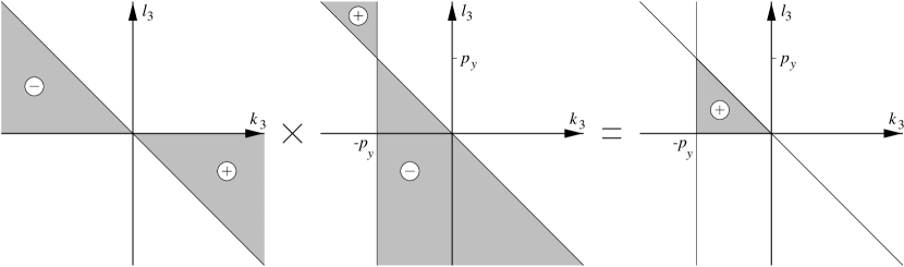
Figure 2: Constraints after the $l_{2}$- and the $k_{2}$-integrations

E.g. when we perform the $l_{2}$-integration for a scattering-amplitude of type and apply lemma 1 on all the resulting residues, we obtain the infinite domains sketched on the left of figure 2. (The signs denote the weight of the integrand there and stems from the numerator in (2)). After the $k_{2}$-integration we obtain the domain in the middle and when multiplied, only a finite triangle in the $k_{3}$-$l_{3}$-plane remains.

Performing the $l_{1}$- and the $k_{1}$-integrations in the same way we encounter poles on the real axis. They are, however, purely artificial and a consequence of choosing equal imaginary parts $\eta$ in all propagators. Treating the integral as a Cauchy Principal Value integral, the residue theorem can still be applied in these cases since there are only odd coefficients in the integrand’s Laurent-series but the residue contributes only with a weight $\pi i$ instead of $2\pi i$ [13].

When this procedure is continued and all the constraints are combined applying both lemmata, we get the 6 domains of integration in the $k_{0}$-$l_{0}$-plane shown in figure 3 for a

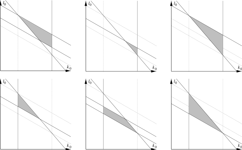
Figure 3: Constraints after the $l_{1}$- and the $k_{1}$-integrations in topology I b). The exact parameters of the borders are functions of $k_{3}$ and $l_{3}$.

scattering-amplitude . (There are only 6 domains remaining instead of 9 due to an incompatibility of constraints after the $l_{2}$- and the $k_{2}$-integrations in 3 of them.) The exact parameters of the borders of these domains depend on $k_{3}$ and $l_{3}$. We emphasize again, that the resulting domains of integration in the edge variables are always finite and bounded by linear functions—even in the case of crossed topologies—thus making them accessible to an unambiguous reparametrization and subsequent next integration. In the case of crossed topologies, lemma 2 can be applicable more than twice because of the presence of two mixed propagators. The numbers of remaining terms turn out to be 12 in and 5 in .

3 Towards a 3-dimensional Integral

The procedure outlined above produces a 4-fold integration of rational function over a finite volume in the edge variables:

$$\int_{l_{3}^{(u)}}^{l_{3}^{(o)}}\!\!dl_{3}\int_{k_{3}^{(u)}}^{k_{3}^{(o)}}\!\!dk_{3}\int_{l_{0}^{(u)}}^{l_{0}^{(o)}}\!\!dl_{0}\int_{k_{0}^{(u)}}^{k_{0}^{(o)}}\!\!dk_{0}\,\frac{P(l_{0},k_{0},l_{3},k_{3})}{Q(l_{0},k_{0},l_{3},k_{3})}.$$ (8)

The appearance of a numerator containing integration variables is due to the solutions of $P=0$ with respect to middle variables inserted into the remaining propagators. After partial-fractioning this integrand can always be transformed into one, where $Q$ is no more than quadratic in the edge variables. The integration-domains in the $k_{0}$-$l_{0}$-plane which depend on $k_{3}$ and $l_{3}$ can be mapped into some fixed domain independent of $k_{3}$ and $l_{3}$ using a suitable linear transformation. The rational function can then be integrated once more, resulting in other rational functions, logarithms and arcustangens where care has to be taken of the small imaginary part and the position of branch-cuts. The coefficients of the result will generally involve square roots of quartic functions in the remaining three variables. This three-dimensional integration should be accessible to numerical evaluation using vegas [15, 16, 17] or similar routines.

4 An Example

We will now test our method on a simple example: a decay-amplitude of type where a heavy scalar particle decays into a lighter and two massless ones as shown in figure 4. The choice of momentum-flow indicated there results in the inverse propagators

$$P_{l,1}=l^{2}-m_{1}^{2}+i\eta, P_{l,2}=(l+p_{3})^{2}-m_{2}^{2}+i\eta,$$

$$P_{k,3}=(k-p_{1}+p_{2})^{2}-m_{3}^{2}+i\eta, P_{k,4}=(k-p_{1})^{2}-m_{4}^{2}+i\eta,$$

$$P_{l+k,5}=(l+k)^{2}-m_{5}^{2}+i\eta.$$ (9)

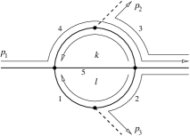
Figure 4: Choice of momentum-flow for a decay-process of type III b)

The most convenient Lorentz frame for this case turns out not to be the rest-frame of the decaying particle but the one in which the 3-momenta of the light-like particles are antiparallel and aligned to a specific coordinate-axis, say $x$. This frame can always be reached by a Lorentz transformation as long as the two light-like particles do not have equal momenta.

When integrating out the middle variables with these conditions and applying the rules found in section 2 one finds, however, incompatible constraints in the $l_{1}$- and the $k_{1}$-integrations. To get out of the dilemma, the light-cone condition for the two massless external particles must be temporarily relaxed. A possible choice of momenta is

$$p_{1}^{\mu}=(q_{\eta},p_{x},p_{y},0),\quad p_{2}^{\mu}=(q_{\gamma},q_{x},0,0),\quad p_{3}^{\mu}=(q_{\gamma},-q_{x},0,0),$$

$$p_{4}^{\mu}=p_{1}^{\mu}-p_{2}^{\mu}-p_{3}^{\mu}=(q_{\eta}-2\,q_{\gamma},p_{x},p_{y},0),$$ (10)

where $q_{\gamma}=\lim_{\epsilon\rightarrow+0}q_{x}+\epsilon$ is tacitly assumed.

Now the integrations in the middle variables can be performed resulting in the domain of figure 5 for the $k_{0}$- and the $l_{0}$-integrations in addition to the one already known from figure 2 for the $k_{3}$- and $l_{3}$-integrations.

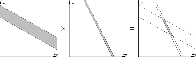
Figure 5: Constraints after the $l_{1}$- and the $k_{1}$-integrations in topology III b)

If we use a linear transformation in the $k_{0}$-$l_{0}$-plane in order to map this domain into a unit-square $\tilde{k}_{0}=(0\dots 1)$, $\tilde{l}_{0}=(0\dots 1)$, another one to map the triangle in the $k_{3}$-$l_{3}$-plane into a unit-triangle $\tilde{k}_{3}=(0\dots 1)$, $\tilde{l}_{3}=(0\dots 1-\tilde{k}_{3})$, the limit $\epsilon\rightarrow 0$ can safely be performed and we obtain the representation

$$V(p_{1},p_{2},p_{3})={}-(2\pi i)^{4}\int_{0}^{1}\!\!\!d\tilde{k}_{3}\int_{0}^{1-\tilde{k}_{3}}\!\!\!\!d\tilde{l}_{3}\,\int_{0}^{1}\!\!\!d\tilde{k}_{0}\int_{0}^{1}\!\!\!d\tilde{l}_{0}\,\frac{1}{(b_{1}\,\tilde{k}_{0}+b_{0})\,\tilde{l}_{0}+(a_{1}\,\tilde{k}_{0}+a_{0})+\,i\eta}$$ (11)

where the coefficients are given by

$$a_{0} = 16\,\left(\tilde{k}_{3}\,\tilde{l}_{3}\,m_{5}^{2}\big{/}(\tilde{l}_{3}+\tilde{k}_{3}-1)-\tilde{k}_{3}\,m_{1}^{2}-\tilde{l}_{3}\,m_{3}^{2}\right.$$

$$\left.\quad{}-\tilde{k}_{3}\,\tilde{l}_{3}\,\bigl{(}p_{x}^{2}+p_{y}^{2}-q_{\eta}^{2}+2\,q_{\gamma}\,(q_{\eta}-p_{x})\bigr{)}\right),$$

$$a_{1} = 16\,\tilde{l}_{3}\,\bigl{(}2\,q_{\gamma}\,\tilde{k}_{3}\,(q_{\eta}-p_{x})+m_{3}^{2}-m_{4}^{2}\bigr{)},$$ (12)

$$b_{0} = 16\,\tilde{k}_{3}\,\bigl{(}2\,q_{\gamma}\,\tilde{l}_{3}\,(2\,q_{\gamma}-q_{\eta}-p_{x})+m_{1}^{2}-m_{2}^{2}\bigr{)},$$

$$b_{1} = -64\,\tilde{k}_{3}\,\tilde{l}_{3}\,q_{\gamma}^{2}.$$

In this case, all terms quadratic in $\tilde{l}_{0}$ or $\tilde{k}_{0}$ in the denominator have canceled, allowing for an integration in both of these variables. Splitting the integral into Principal Value integral and $\delta$-function separates real- and imaginary part. We obtain a numerically stable two-fold representation with dilogarithms in the real part and logarithms in the imaginary part which displays the correct behaviour even at thresholds.

By letting $q_{\gamma}\rightarrow 0$ we restrict our kinematical regime even further and obtain a two-point sunset-topology with two propagators squared. Numerical stability, however, breaks down as we approach this limit. A look at the arguments of the dilogarithms in our two-dimensional representation expanded in small $q_{\gamma}$ reveals why:

$$\lim_{q_{\gamma}\rightarrow 0}\operatorname{Re}\big{(}V(p_{1},p_{2},p_{3})\big{)}=\operatorname{Re}\big{(}P(p_{1}^{2})\big{)}=-(2\pi i)^{4}\!\int_{0}^{1}\!\!\!d\tilde{k}_{3}\int_{0}^{1-\tilde{k}_{3}}\!\!\!\!d\tilde{l}_{3}$$ (13)

$$\frac{1}{64\,\tilde{k}_{3}\,\tilde{l}_{3}\,q_{\gamma}^{2}}\;\operatorname{Re}\left(\operatorname{Li_{2}}(1+\hat{r}_{24}\,q_{\gamma}^{2})-\operatorname{Li_{2}}(1+\hat{r}_{23}\,q_{\gamma}^{2})-\operatorname{Li_{2}}(1+\hat{r}_{14}\,q_{\gamma}^{2})+\operatorname{Li_{2}}(1+\hat{r}_{13}\,q_{\gamma}^{2})\right).$$

The coefficients in this formula are

$$\hat{r}_{ij} = \frac{4\,\tilde{k}_{3}\,\tilde{l}_{3}\,p_{1}^{2}}{(m_{3}^{2}-m_{4}^{2})(m_{1}^{2}-m_{2}^{2})}$$ (14)

$${}+4\,\frac{(\tilde{k}_{3}\,m_{i}^{2}+\tilde{l}_{3}\,m_{j}^{2})\,(1-\tilde{k}-\tilde{l})\,+\,m_{5}^{2}\,\tilde{l}_{3}\,\tilde{k}_{3}}{(m_{3}^{2}-m_{4}^{2})(m_{1}^{2}-m_{2}^{2})(\tilde{k}_{3}+\tilde{l}_{3}-1)}.$$

with $p_{1}^{2}=q_{\eta}^{2}-p_{x}^{2}-p_{y}^{2}$ as the only combination of exterior momenta (c.f. eq. (4)) entering $P$, as it should be.

Numerical stability can be restored in (13) if the expansion of the dilogarithms at their branch-point as generalized Taylor series

$$\operatorname{Re}\left(\operatorname{Li_{2}}(1+\epsilon)\right)=\frac{\pi^{2}}{6}+\epsilon(1-\ln|\epsilon|)+O(\epsilon^{2})$$

and the relation $\hat{r}_{24}-\hat{r}_{23}-\hat{r}_{14}+\hat{r}_{13}=0$ are used.

We compare this with numerical results obtained via another method [14] and find agreement below and above threshold (figure 6). (For definiteness, all masses have been chosen equal, requiring yet another expansion due to the denominators in (14).)

Figure 6: Comparison of our method with a calculation of the scalar sunset-graph with two squared propagators of mass $m$. (Diamonds represent numerical results from our calculation.)

5 Conclusion

The method for calculating scalar 2-loop box-functions with arbitrary internal masses proposed in [1] turns out to deliver a moderate number of 4-dimensional integrals, which can always be reduced further to 3-dimensional representations—in some cases even 2-dimensional ones. In sample-cases we have been able to produce reasonable numerical results in arbitrary kinematical regimes below and above threshold. In the limit of limiting kinematical points, numerical stability is lost but can be restored by expanding the representation around that point. We hope to obtain similar results for all the 5 genuine 2-loop box-functions and incorporate them into xloops [10].

6 Acknowledgements

R. Kreckel is grateful to the ‘Graduiertenkolleg Elementarteilchenphysik bei hohen und mittleren Energien’ at University of Mainz for supporting part of this work. D. Kreimer thanks Bob Delbourgo and the Physics Dept. at the Univ. of Tasmania for hospitality during a visit in March 1998 and the DFG for support.

References

- [1] D. Kreimer: A short note on two-loop box functions; Phys. Lett. B347 (1995) 107; hep-ph/9407234.
- [2] T. Kinoshita: Theory of the Anomalous Magnetic Moment of the Electron—Numerical Approach; published in: Kinoshita (ed.): Quantum Electrodynamics, World Scientific, (1990)
- [3] D. Kreimer: The master two-loop two-point function. The general cases; Phys. Lett. B273 (1991) 277
- [4] D. Kreimer: The two-loop three-point functions: general massive cases; Phys. Lett. B292 (1992) 341
- [5] A. Czarnecki, U. Kilian, D. Kreimer: New representation of two-loop propagator and vertex functions; Nucl. Phys. B433 (1995) 259
- [6] A. Frink, U. Kilian and D. Kreimer: New representation of the two-loop crossed vertex function; Nucl. Phys. B488 (1997) 426; hep-ph/9610285
- [7] A. I. Davydychev, J. B. Tausk: Two-loop self-energy diagrams with different masses and the momentum expansion; Nucl. Phys. B397 (1993) 123
- [8] J. Fleischer, M. Tentyukov: Methods to calculate scalar two-loop vertex diagrams; hep-ph/9802244
- [9] B. G. Nickel: Evaluation of simple Feynman graphs; J. Math. Phys. 19 (1978) 542
- [10] L. Brücher, J. Franzkowski, A. Frink, D. Kreimer: Introduction to XLOOPS; hep-ph/9611378
- [11] C. Itzykson, J.B. Zuber: Quantum Field Theory; World Scientific Lecture Notes in Physics (1993)
- [12] H. Cartan: Théorie Élémentaire des Fonctions Analytiques d’une ou plusieurs Variables Complexes; Hermann, Paris, (1963)
- [13] M. J. Ablowitz, A. S. Fokas: Complex Variables; Cambridge University Press (1997)
- [14] P. Post, J. B. Tausk: The sunset diagram in SU(3) chiral perturbation theory; hep-ph/9604270.
- [15] G. P. Lepage: A New Algorithm for Adaptive Multidimensional Integration; J. Comput. Phys. 27 (1978) 192
- [16] G. P. Lepage: VEGAS—An Adaptive Multi-dimensional Integration Program; Publication CLNS-80/447, Cornell University (1980)
- [17] R. Kreckel: Parallelization of adaptive MC integrators; Comp. Phys. Comm. 106 (1997) 258; physics/9710028