LAL 98-16

$C\!P$ violation with B AB AR

Stéphane Plaszczynski

Laboratoire de l’Accélérateur Linéaire,
IN2P3-CNRS et Université de Paris-Sud, F-91405 Orsay

The B A B AR experiment is a new generation detector located at the SLAC B factory PEP-II ring which should start taking data at the end of 1999. Its main goal is the study of $C\!P$ violation in the $B^{0}\overline{B}{}^{0}$  system. After explaining the nature of this $C\!P$ violation, I review the scientific program for achieving this study in many different modes, in the light of the recent developments obtained both on the experimental and theoretical side. Implications for the Standard Model are then discussed.

Invited talk at the $XII^{th}$ Rencontres de physique de la Vallée d’Aoste, la Thuile, Italy, March 1-7 1998

1 Introduction

So far the violation of $C\!P$ symmetry has just been observed in the neutral Kaon sector. The Standard Model can accommodate for such a violation, through the CKM mixing matrix. Furthermore, it even predicts $C\!P$violation in the $B^{0}\overline{B}{}^{0}$  system. A first task of a B factory is thus to check whether such a prediction holds on in the $B^{0}$  sector.

The CKM matrix is presently one of the less tested sector of the Standard Model. Indeed, two of its four parameters are presently very badly known ( $\rho$ and $\eta$ in the Wolfenstein parametrization). The knowledge on these two parameters is depicted in the so-called Unitarity Triangle (UT), where the apex of the scaled triangle is precisely the $\rho,\eta$ point (Fig 1).

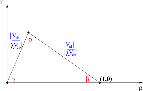
Figure 1: The Unitarity Triangle representation. Note that its base is normalized to 1

Presently the three sides of the triangle are measured, but the extraction from the data of CKM quantities requires the knowledge of model-dependent theoretical parameters (coming from non-perturbative QCD and models for heavy to light transitions). Another constraint comes from the measurement of $C\!P$ violation in the kaon system, but here again, due to large theoretical uncertainties, this constraint is quite weak. The use of limits on the $B_{s}$ mixing frequency is interesting but again plagued by a theoretical parameter (section 5.1).

The goal of B factories is to measure two angles of the UT ($\alpha$ and $\beta$) in a clean way. Combining all observables will allow to (over-?)constrain the CKM matrix. Furthermore, time dependent $C\!P$ violating asymmetries, being rare processes, are sensitive to New Physics phenomenon. Or, said in another way, many extensions of the Standard Model includes some new sources of $C\!P$ violation [1] that could be observed at a B-factory experiment.

2 Which $C\!P$ violation?

In the $\Upsilon{\rm(4S)}\rightarrow B^{0}\overline{B}{}^{0}$  decay, after the decay of a tagging flavor B, the time distribution of the decay of the other B (to a final state $f$) is of the form:

$$\rho(t) = Ce^{-\Gamma t}[1+|{\lambda_{f}}|^{2}{+}(1-|{\lambda_{f}}|^{2}){\cos({\Delta{m}_{d}}t)}{-}2Im{\lambda_{f}}{\sin({\Delta{m}_{d}}t)}]~{}\mbox{($B^{0}$tag)}$$

$$\bar{\rho}(t) = Ce^{-\Gamma t}[1+|{\lambda_{f}}|^{2}{-}(1-|{\lambda_{f}}|^{2}){\cos({\Delta{m}_{d}}t)}{+}2Im{\lambda_{f}}{\sin({\Delta{m}_{d}}t)}]~{}\mbox{($\overline{B}{}^{0}$tag)}$$ (1)

where ${\lambda_{f}}=\frac{q}{p}\frac{{\cal A}(\overline{B}{}^{0}\rightarrow f)}{{\cal A}(B^{0}\rightarrow f)}$ , ${\Delta{m}_{d}}$ is the $B_{d}$ mixing frequency and $\Gamma$ its width. One notices the difference in signs in the above expression.

Choosing a final $C\!P$  eigenstate, the time dependent asymmetry $a(t)$ can be different from 0, indicating $C\!P$  violation:

$$a(t)=\frac{N(B^{0}(t)\rightarrow f)-N(\overline{B}{}^{0}(t)\rightarrow{f})}{N(B^{0}(t)\rightarrow f)+N(\overline{B}{}^{0}(t)\rightarrow{f})}=\frac{(1-|{\lambda_{f}}|^{2}){\cos({\Delta{m}_{d}}t)}-2Im{\lambda_{f}}{\sin({\Delta{m}_{d}}t)}}{(1+|{\lambda_{f}}|^{2})}$$ (2)

There are two ways for the ratio to be non zero:

• $|{\lambda_{f}}|\neq 1$
  This can be achieved either by $|\frac{q}{p}|\neq 1$ or $\frac{{\cal A}(\overline{B}{}^{0}\rightarrow f_{CP})}{{\cal A}(B^{0}\rightarrow f_{CP})}\neq 1$. The former inequality represents a $C\!P$ violation in the mixing (indirect) and the latter a $C\!P$ violation in the decay (direct). The amount of indirect $C\!P$ violation is expected to be very small in the $B^{0}\overline{B}{}^{0}$ system (at a level of $10^{-3}$). Direct $C\!P$ violation however can be different from 0 in rare processes (beyond tree diagrams) and depends on the modes studied.

• $Im{\lambda_{f}}\neq 0$
  The term $Im{\lambda_{f}}$ has no reason to be equal to 0. In some “clean” cases it can even be directly related to the angles of the Unitarity Triangle: $Im{\lambda_{f}}=\sin 2\alpha$ or $Im{\lambda_{f}}=\sin 2\beta$. It arises from the interference between the decay with and without mixing. It is the prime motivation for the construction of B-factories.

3 Introducing B A B AR

To achieve an experimental study of such time dependent asymmetries, the following requirements must be fulfilled:

• produce a coherent $B^{0}\overline{B}{}^{0}$state (i.e. run a the $\Upsilon{\rm(4S)}$resonance).

• since CP modes are rare (BR of the order of $10^{-4},10^{-5}$) have a high luminosity,

• the time variable that appears in Eq.(2) being the decay time between the two B decays ($t=\Delta t$), it is crucial that they do not decay at the same point (otherwise the ${\sin({\Delta{m}_{d}}t)}$ term cannot be measured in a time dependent way and the time-integral over this term vanishes): one needs therefore to boost the $B^{0}\overline{B}{}^{0}$  system, i.e. use asymmetric beams.

The B A B AR detector is located at the PEP-II storage ring, a high luminosity collider (${\cal L}=3.10^{33}cm^{-2}s^{-1}$ is expected) of 9  GeV electrons against 3.1  GeVpositrons. This gives a boost to the $B^{0}\overline{B}{}^{0}$ system of $\gamma\beta=0.56$; the mean separation between the two B decays is about $260\,\mu\mbox{m}$.

The (asymmetric) detector is a classical one for $e^{+}e^{-}$ colliders (except for the DIRC), made of high quality components. Going from the beam pipe (Fig 2):

• a 5 layer silicon vertex tracker

• a low density He-based Drift chamber

• a CsI(Tl) calorimeter with high granularity.

• a DIRC (Detection of Internally Reflected Cerenkov light) for particle identification

• a superconducting coil of 1.5 T.

• An instrumented flux return optimized for $\mu$ and $K^{0}_{\scriptscriptstyle L}$ detection.

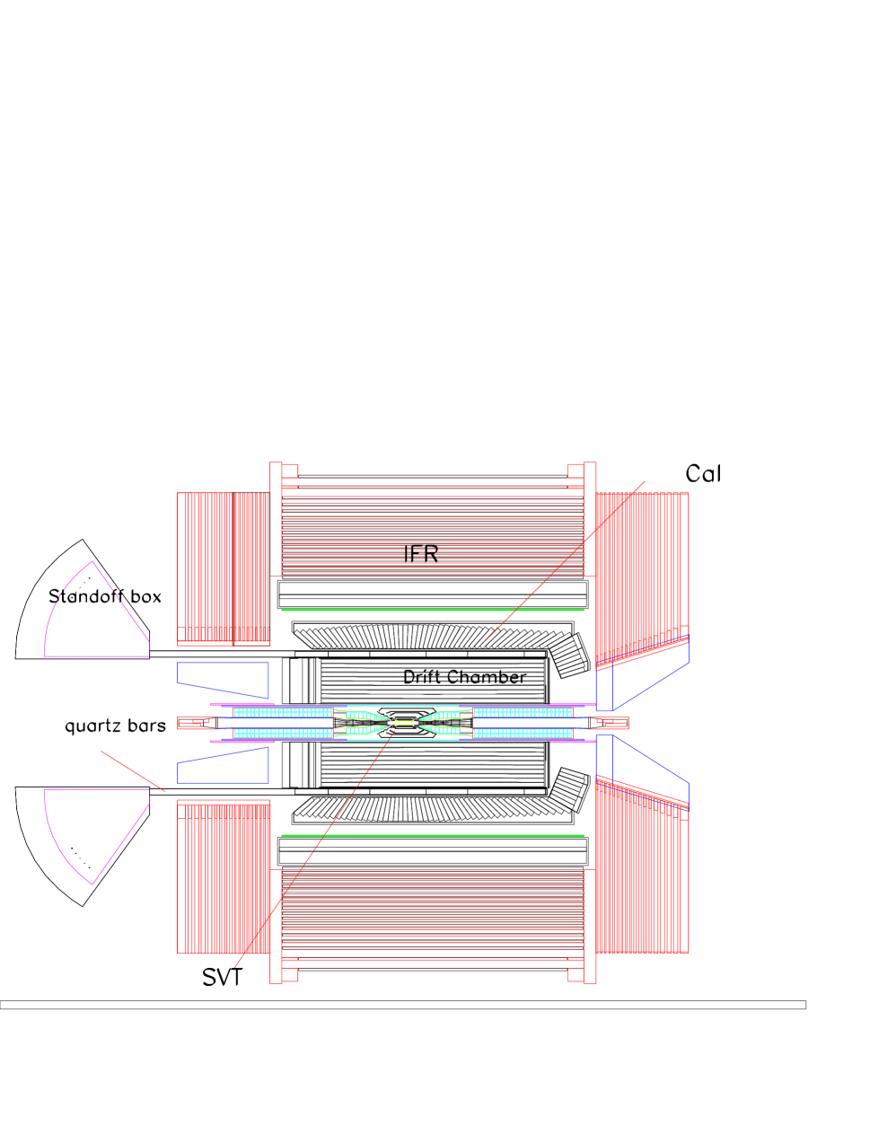
Figure 2: Sketch of the B A B AR detector

The DIRC is a new detector for Particle Identification based on the Cerenkov light emission of a particle passing through a quartz bar. While generally the light captured in the radiator is lost, here one uses this component which is trapped inside the quartz bar and propagate by internal reflection to the end, conserving its characteristic angle. At the end of the bar, the photon propagates into a large volume of water (the “standoff box”) and reaches a huge array of about 13 000 photomultipliers. The reconstruction of the angle between the hit PMT and the bar allows to measure the Cerenkov angle, and thus the nature of the track.

4 The $C\!P$ program

In order to extract $C\!P$  violation parameters, one needs in real life to perform the following program:

4.1 Reconstruction of a final state $f$

This is performed by usual techniques (mass peaks…), for many different final states:

$$f={J\mskip-3.0mu/\mskip-2.0mu\psi\mskip 2.0mu}K^{0}_{\scriptscriptstyle S},~{}\pi^{+}\pi^{-},~{}\pi^{+}\pi^{-}\pi^{0},~{}4\pi,D^{+}D^{-},{J\mskip-3.0mu/\mskip-2.0mu\psi\mskip 2.0mu}K^{\ast},D^{\ast+}D^{\ast-},\psi(2S)K,..$$ (3)

I will detail the first three modes while describing the following of the analysis.

4.2 Tagging

The goal of this part is to tag the flavor of the B meson ($b$ or $\bar{b}$ quark?). This is generally performed searching for a lepton and/or kaon in the event (Fig. 3)

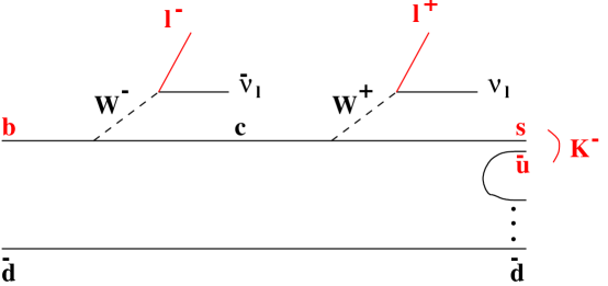
Figure 3: Ways to produce a lepton and a kaon in a $\overline{B}{}^{0}$decay

A sign contamination comes from secondary leptons; usually one uses a cut (as on its momentum) to enrich the sample in primary leptons. However in that case, one looses the information contained in the secondary leptons: if it is very soft, it is more likely to be a secondary lepton, so its sign information should be flipped.

A tool named $CORNELIUS$ [11] has been developed in the Collaboration, in order to combine the information of many discriminating variables associated to the lepton. This is achieved using various multivariate methods ; it allows to crosscheck the different outputs and have a grip on systematics. But much more. It allows to assign to each event a probability to come from a $b$ or $\bar{b}$ quark. This probability is then input in the final likelihood determining the asymmetry and exploits optimally all the available information.

The deterministic “cut” method degrades the determination on the asymmetry by a dilution $D=\epsilon(1-2\mbox{w}^{2})$ where $\epsilon$ is the tagging fraction and w the mistag fraction. Previous estimates of this quantity [2] gave about: $D=0.33$. Using the probability method allows to reach $D=0.41$, by combining 8 discriminating variables for the lepton.

Notice that this combination can also be used to reject the background (generally “continuum background”) by combining discriminating variables based on the event topology. $CORNELIUS$ can provide event by event a probability to be a $B\bar{B}$ or $q\bar{q}$ event.

4.3 Time determination

Once a mode is reconstructed, a vertex is performed with the remaining charged tracks. The difference in space between both vertices represents simply $\gamma\beta ct$ where $\gamma\beta$ is the known boost of the machine (=0.56). The resolution on the distance between both vertices is, for the ${J\mskip-3.0mu/\mskip-2.0mu\psi\mskip 2.0mu}$$K^{0}_{\scriptscriptstyle S}$ mode, about 50$\,\mu\mbox{m}$, well beyond the mean $260\,\mu\mbox{m}$ quoted in section 3 for the mean B separation.

4.4 Extracting $C\!P$

There are two aspects in extracting a quantity relevant for physics. The first one is mainly experimental and is based on the knowledge of the detector. It will be illustrated on the ${J\mskip-3.0mu/\mskip-2.0mu\psi\mskip 2.0mu}K^{0}_{\scriptscriptstyle S}$ mode. Going from a measured asymmetry to a relevant CKM quantity is a more theoretical problem, that will be illustrated on the $\pi^{+}\pi^{-}$ mode.

4.4.1 Experimental side: introducing the $\cal KIN$ variable (${J\mskip-3.0mu/\mskip-2.0mu\psi\mskip 2.0mu}$$K^{0}_{\scriptscriptstyle S}$)

The extraction of the asymmetry can be performed by a likelihood fit to the observed events. However it is more convenient to use the $\cal KIN$ variable.

In a simple case (the theoretically clean mode :${J\mskip-3.0mu/\mskip-2.0mu\psi\mskip 2.0mu}K^{0}_{\scriptscriptstyle S}$) and neglecting for the time being detector effects, the event distributions (2) can be written:

$$B^{0}~{}tag:\rho(t) = Ce^{-\Gamma t}[1{-}\sin 2\beta{\sin({\Delta{m}_{d}}t)}]$$

$$\overline{B}{}^{0}~{}tag:\bar{\rho}(t) = Ce^{-\Gamma t}[1{+}\sin 2\beta{\sin({\Delta{m}_{d}}t)}]$$ (4)

Constructing event by event the asymmetry

$$S_{tag}\frac{\rho-\bar{\rho}}{\rho+\bar{\rho}}~{}=S_{tag}{\sin({\Delta{m}_{d}}t)}\sin 2\beta=\dot{\kappa}\sin 2\beta$$ (5)

(where $S_{tag}=\pm 1$ for $B_{0}$${\scriptscriptstyle(}{\scriptstyle-}{\scriptscriptstyle)}$  tag) allows to fill an histogram of the $\cal KIN$ ($\dot{\kappa}$) variable (see Fig 4).

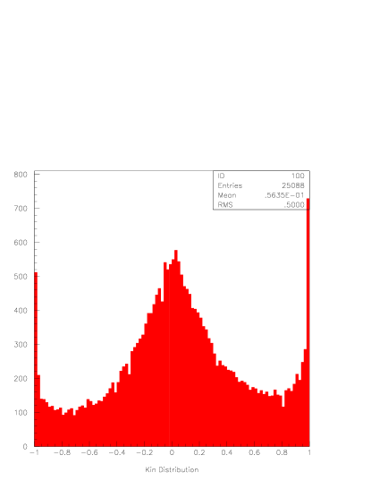
Figure 4: An example of the $\cal KIN$ distribution on ${J\mskip-3.0mu/\mskip-2.0mu\psi\mskip 2.0mu}K^{0}_{\scriptscriptstyle S}$ mode. From the upper box, one can get the whole information on the determination of $\sin 2\beta$

The distribution of $\dot{\kappa}$ variable has the nice property that, to a very good approximation, one can get the estimate of the asymmetry ($\sin 2\beta$) by the very simple formula [3]:

$$\sin 2\beta\simeq\frac{\langle\dot{\kappa}\rangle}{\langle\dot{\kappa}^{2}\rangle}\pm\frac{1}{\sqrt{N\langle\dot{\kappa}^{2}\rangle}}$$ (6)

This means that a single plot (as Fig 4) carries the whole asymmetry information, and that the asymmetry measurements can be obtained via the number of entries, the mean and the RMS of this histogram. Furthermore one can incorporate in the $\cal KIN$ , the tagging probability event by event and the time resolution measurement [3]. All the $\cal KIN$ results still hold. Finally notice, that the different modes can be combined in a straightforward way by just summing the $\dot{\kappa}$ histograms.

Using the $\cal KIN$ approach , a recent analysis of the ${J\mskip-3.0mu/\mskip-2.0mu\psi\mskip 2.0mu}$$K^{0}_{\scriptscriptstyle S}$mode has been performed [4]. The measurement obtained for $30fb^{-1}$ (one “nominal” year) is: $\sin 2\beta=0.82\pm 0.15$ (while .70 was generated).

4.4.2 Theoretical side: the penguin world ($\pi^{+}\pi^{-}$)

Contributing to a final state as $\pi^{+}\pi^{-}$, can exist, beside the Tree Cabbibo suppressed mode (a), some modes as “penguin diagrams”(b). Recently emphasis has also been put on “long distance penguins”(c) (or “charming” penguins) which are of QCD non-perturbative nature and results from annihilation/re-scattering processes.

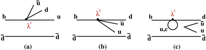
Figure 5: Possible contributions to the $\pi^{+}\pi^{-}$ mode, in term of local 4-fermion operators: (a) tree (b)penguin (c) “charming” penguin

The theoretical estimate of the penguin contribution is very delicate (and model-dependent). For this mode, it is expected that the penguin contribution is “smaller” than the Tree one. However, recent CLEO measurements of $BR(B^{0}\rightarrow K\pi)$ [5] indicates that these penguin modes indeed exist and should not be neglected in extracting the CKM quantity $\sin 2\alpha$.

Under the influence of penguins, the time distribution of the events Eq.(2) can be written as:

$$Ce^{-\Gamma t}(1\pm{R}{\cos({\Delta{m}_{d}}t)}\mp\sin 2({\alpha+\delta}){\sin({\Delta{m}_{d}}t)})$$ (7)

where $R$ is the amount of direct $C\!P$ violation, $\delta$ is a shift due to the presence of penguins and $\alpha$ is the CKM angle.

What one can extract from the data is a $\sin 2\alpha_{eff}$ but the penguin shift is unknown. There are several solutions to this problem, depending on what will be measured:

• Gronau and London [6] have shown that measuring the decoupled amplitudes:

  $$A(B^{0}\rightarrow\pi^{+}\pi^{-}) A(\overline{B}{}^{0}\rightarrow\pi^{+}\pi^{-})$$ ,

  $$A(B^{+}\rightarrow\pi^{+}\pi^{0}) A(B^{-}\rightarrow\pi^{-}\pi^{0})$$ , (8)

  $$A(B^{0}\rightarrow\pi^{0}\pi^{0}) A(\overline{B}{}^{0}\rightarrow\pi^{0}\pi^{0})$$ ,

  allows to extract $\alpha$ by using the isospin symmetry. This is however performed with an 8-fold ambiguity on $2\alpha$. Furthermore, the amplitudes of the $\pi^{0}\pi^{0}$ mode are expected to be small (color suppressed) and experimentally difficult to reconstruct.

• In the case where only an upper bound has been obtained for this $\pi^{0}\pi^{0}$ mode, Grossman and Quinn [7] have shown that the penguin shift is limited by:

  $${\sin^{2}\delta}\leq\frac{BR(B^{0}\rightarrow\pi^{0}\pi^{0})+BR(\overline{B}{}^{0}\rightarrow\pi^{0}\pi^{0})}{BR(B^{+}\rightarrow\pi^{+}\pi^{0})+BR(B^{-}\rightarrow\pi^{-}\pi^{0})}$$ (9)

  This can be very useful when constraining the penguin effects.

• Finally one will have to rely on the theorist understanding of the penguin , reducing the model-dependence to a minimum number of parameters [8], to obtain a systematic error on the determination of $\sin 2\alpha$.

4.4.3 The full problem: $\pi^{+}\pi^{-}\pi^{0}$

A clearly challenging mode to extract $\alpha$ is $\pi^{+}\pi^{-}\pi^{0}$. In that case the situation is complicated by the fact that:

• $\rho-\pi$ is assumed to dominate but $\rho^{+}\pi^{-},\rho^{-}\pi^{+},\rho^{0}\pi^{0}$ interferes.

• Experimentally the signal is not so pure (signal:background $\simeq$ 1:1)

• There is a unknown contribution from penguins.

However this mode is important since, it is expected to have a higher branching ratio than $\pi^{+}\pi^{-}$. Also since it is a non-CP final state (due to phase space) it can have a large ${\cos({\Delta{m}_{d}}t)}$ contribution, leading to a simultaneous determination of $\cos 2\alpha$ and $\sin 2\alpha$. This would definitely reduce the ambiguities due to a single measurement of $\sin 2\alpha$ (in which case $2\alpha=\arcsin(\sin 2\alpha)$ and $2\alpha=\pi-\arcsin(\sin 2\alpha)$ are both solutions).

The observed asymmetry in this case is of the form:

$$Ce^{-\Gamma t}[1\pm{b(\Phi)}{\cos({\Delta{m}_{d}}t)}\mp{c(\Phi)}{\sin({\Delta{m}_{d}}t)}]$$ (10)

where $b(\Phi),c(\Phi)$ are functions of the phase space (as the 2 Dalitz plot coordinates).

If one collects enough data, the study of the time-dependent Dalitz plot allows to fit $b(\Phi),c(\Phi)$ and extract from the data all the information on $\alpha$ and penguin contributions [9]. This requires however a large statistics, and as in the $\pi^{+}\pi^{-}$ case, the measurement of the color suppressed contribution (here $\rho^{0}\pi^{0}$) is mandatory. Based on some models for the branching ratios [8] , this could require about 3 years of data taking.

In the first year(s), the approach to this problem will be a 2 body approach: phase space is integrated , using relativistic Breit-Wigner, and taking into account interferences between $\rho^{+}\pi^{-}$ and $\rho^{-}\pi^{-}$. The effects of the penguins are neglected and will induced a systematic error. A recent analysis of this channel [10] obtains, for one year of data taking, an effective asymmetry: $\sin 2\alpha_{eff}=0.26\pm 0.15(stat)$ while the generated value (with penguins) was 0.43. This can give an idea of the induced penguin shift.

Notice however that for this mode, as for $\pi^{+}\pi^{-}$ very much depends on what the different measured branching ratios will be.

4.4.4 Modes studied in B A B AR

So far, I have just described 3 analyzes. Many more channels are in fact studied and Table 1 summarizes the different modes which allow a determination of the angles $\beta$ and $\alpha$ of the Unitarity Triangle.

Angle	Mode	quark process	penguins
$\beta$	Charmonium $K^{0}_{\scriptscriptstyle S}(K^{0}_{\scriptscriptstyle L}?)$	$b\rightarrow c\bar{c}s$	$|P|\ll|T|$
	Charmonium $K^{\ast}$
	$D^{+}D^{-},~{}D^{\ast+}D^{\ast-},DD^{\ast}$	$b\rightarrow c\bar{c}d$	$\frac{|P|}{|T|}?$
	$\phi K^{0}_{\scriptscriptstyle S}$	$b\rightarrow s\bar{s}s$	$|P|\gg|T|$
$\alpha$	$\pi^{+}\pi^{-}$	$b\rightarrow u\bar{u}d$	$\frac{|P|}{|T|}\leq 1$
	$\pi^{+}\pi^{-}\pi^{0}(\rho\pi)$		$\frac{|P|}{|T|}?$
	$\pi^{+}\pi^{-}\pi^{0}\pi^{0}(a_{1}\pi,\rho\rho)$		$\frac{|P|}{|T|}?$

Table 1: Different modes studied in the Collaboration. The last column indicates the relative contribution between Tree processes and Penguins

5 Implications for the Standard Model

5.1 Present knowledge of the Unitarity Triangle

Assuming the Cabbibo angle is known well enough, the observables that constrain the other 3 parameters of the CKM matrix (i.e. $A,\rho,\eta$ in Wolfenstein parametrization) are:

• $|V_{cb}|$ which is a direct measurement of $A$. A lot of effort both on theoretical side (to understand corrections to HQET) and experimental side has been invested [12]. The present knowledge is (conservatively)[12] $|V_{cb}|=0.039\pm 0.003$

• $|\frac{{V}_{ub}}{V_{cb}}|$ is obtained from the exclusive or inclusive study of $b\rightarrow u$ decay. In these heavy to light transitions, the theoretical ground is much less firm. Even with a limited sample, the model-dependent error dominates and it is reasonable to assume for it a relative error as large as 25%.

• ${\Delta{m}_{d}}$ (the $B_{d}$ mixing frequency) which is a measurement of $|V_{tb}V_{td}|$. It is now well known thanks to the LEP time-dependent measurements [13]. In order to extract a relevant CKM quantity, one needs to know the theoretical parameter $f_{B_{d}}\sqrt{B_{B_{d}}}$ [15]. There exists a large spread of estimates for this value depending on the model used (lattices, QCD sum rules, quark models…). A reasonable range for these estimates is $f_{B_{d}}\sqrt{B_{B_{d}}}\in[160,240]\mbox{\,Me\kern-0.80002ptV}$

• ${\Delta{m}_{s}}$. LEP provided stringent constraints on the mixing frequency for the $B_{s}$ meson [13]. To extract CKM parameters, one needs in principle to know a parameter analogous to the $B_{d}$ case: $f_{B_{s}}\sqrt{B_{B_{s}}}$. However combined with ${\Delta{m}_{d}}$, knowing the SU(3) flavor correction: $\xi_{s}^{2}=\frac{f_{B_{d}}\sqrt{B_{B_{d}}}}{f_{B_{s}}\sqrt{B_{B_{s}}}}$ is enough. This latter is better known from lattices calculations. Still, recent estimates give: $\xi_{s}^{2}\in[1.12,1.48]$, and not knowing more than that, one must, in order to be conservative, take the upper limit of 1.48. Notice that LEP provided more than a limit (a set of “amplitudes”[13]) and that this information can be used optimally, as exposed in [14].

• $|\varepsilon_{K}|$ is the measurement of indirect $C\!P$ violation in the kaon sector. Here the QCD non-perturbative parameter $B_{K}$ is quite unknown. A reasonable range is: $B_{K}\in[0.6,1.]$

Before combining these observables, let notice that there is a clear part of subjectivity for the theoretical parameters used (depending generally on personal preferences). It is certainly a delicate matter to estimate which model is right, and what the “error” quoted means? An old Bayesian ghost also appears: not knowing which model is right is not the same than taking a flat distribution between all estimates.

B A B AR has adopted the following way of combining , which is statistically meaningful [14]:

The errors on a quantity are divided into 2 types: experimental errors are considered to be gaussianly distributed and enter a $\chi^{2}(A,\rho,\eta)$ estimate. Theoretical parameters are scanned within reasonable ranges: for each scanned parameters, the $\chi^{2}$ is minimized leading to an estimate of $A,\rho,\eta$ and for instance a 95%CL contour in the $\rho-\eta$ plane. A $\chi^{2}$ probability cut is applied in order to check the compatibility between the various observables. If the contour survives, one then go to the next scanned theoretical parameters, etc. Knowing the exact theoretical parameter value, one could fix which contour is the right one. Not knowing it, one takes as a conservative choice the set of all the contours as the overall 95%CL knowledge of $\rho$ and $\eta$. Using this method, the present (1998) knowledge of $\rho-\eta$ is depicted on Fig. 6 (together with the values used).

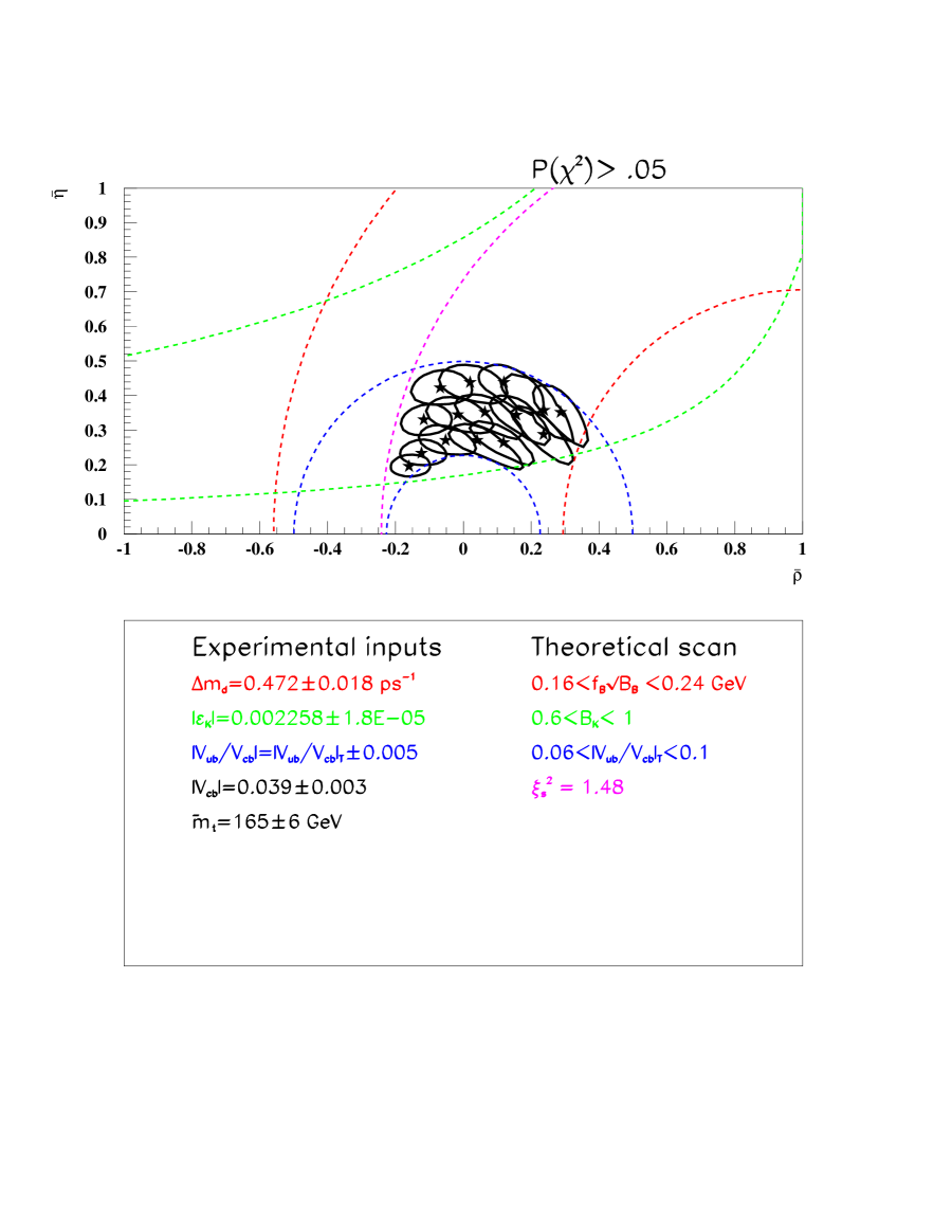
Figure 6: The 1998 knowledge of the $\rho-\eta$: one circle represents the 95% CL obtained when theoretical parameters are fixed. The set of all contours represents our overall 95% knowledge of $\rho\eta$ when scanning the possible range of theoretical parameters. Also drawn in dashed lines are the constraints provides by each individual measurement

Working in another basis ($A,\sin 2\alpha,\sin 2\beta$) , the $\chi^{2}$ minimization can be performed and one obtains in the same way the overall 95% CL in the $\sin 2\alpha,\sin 2\beta$ plane (Fig. 7).

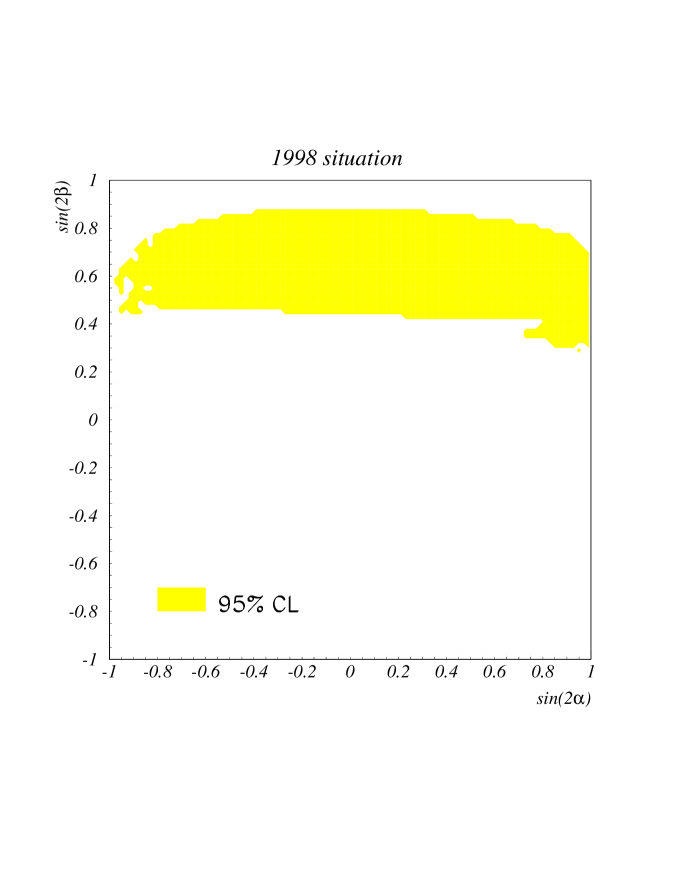
Figure 7: The 1998 knowledge on $\sin 2\alpha-\sin 2\beta$ using the same set of values as in Fig 6

.

From this figure, two important remarks arise:

• $\sin 2\beta$ is presently constrained to lie somewhere on [0.4,0.8](95% CL) . The task of modes measuring $\sin 2\beta$ will therefore to test the Standard Model by checking the compatibility with this range.

• $\sin 2\alpha$ is presently unknown. The goal of a B factory is therefore to measure this angle.

5.2 What a B factory can bring

It is presently quite delicate to foresee what the impact of the B-factory will be in constraining the CKM matrix, since many modes depend on what the branching ratios, penguins, etc.. actually are. B A B AR has updated [11] many of its analyzes with a realistic simulation and the full reconstruction program. A possible scenario for $30fb^{-1}$ integrated luminosity (one year) giving estimated values of these angles is

$$\sin 2\alpha = 0.1\pm 0.1_{exp}\pm 0.2_{th}$$ (11)

$$\sin 2\beta = 0.6\pm 0.08_{exp}$$ (12)

These numbers represent a reasonable order of magnitude but the central values are completely hypothetical (within the Standard Model). Fig 8 shows the impact of such a measurement in the $\rho-\eta$ plane.

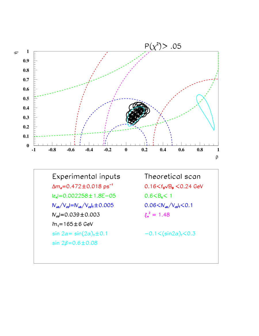
Figure 8: A possible scenario for the determination of $\rho-\eta$ after one year of B A B AR data taking. Also shown as a new contour, in light grey (or blue, in color) is the B A B AR-alone 95% CL.

Two final remarks:

• For this combination one neglects the improvement that will appear with time on the present observables. In particular, $|V_{cb}|,~{}|\frac{{V}_{ub}}{V_{cb}}|,{\Delta{m}_{d}}$ measurements should improve with B-factories.

• Just as knowing the sides of the UT allows to already constrain one of the angle (Fig. 7), in the other way, measuring $\sin 2\alpha$ and $\sin 2\beta$ will allow to measure in a model independent way, the theoretical parameters ($f_{B_{d}}\sqrt{B_{B_{d}}}$, $B_{K}$,$|\frac{{V}_{ub}}{V_{cb}}|_{th}$). This happens on Fig. 8 where the combined contour is not better than the simple B A B AR constraint.

6 Conclusions

Several tools have been developed in the B A B AR collaboration these last years. In particular:

• The tagging is now a probabilistic answer of a multivariate analysis based on discriminating variables. This incorporates optimally the full information extracted from an event.

• The $\cal KIN$ variable is a golden one for the extraction of an asymmetry from the data, modelizing all detector effects. It allows to present results in a clear way, to optimize selections and combine the results of many channels (Collaborations?).

• A method has been developed to combine observables constraining CKM parameters in a statistical meaningful way.

A B-factory will provide precision tests of the Standard Model. First of all, it should prove that $C\!P$ violation exists in the $B^{0}\overline{B}{}^{0}$sector. Then many channels will be combined; this require a deep understanding of the detector. Then, in conjunction with theoretical work, the relevant CKM angles will be extracted.

Presently $\sin 2\beta$ is bound to lie in $[0.4,0.8$](@ 95%CL) from indirect measurements (this however implies the choice of theoretical model-dependent parameters). Therefore the goal of a B factory for this angle is to check whether the time-dependent asymmetry is compatible with this range. The golden modes are Charmonium $K^{0}_{\scriptscriptstyle S}$ and Charmonium $K^{\ast}$. Since these modes are theoretically well under control, any significant deviation from this range would indicate a problem (on errors? theoretical parameters? New Physics?). In particular, if no asymmetry is observed in ${J\mskip-3.0mu/\mskip-2.0mu\psi\mskip 2.0mu}K^{0}_{\scriptscriptstyle S}$ mode, this would rule out the CKM mechanism of mixing between 3 fermion families and indicate New Physics.

Presently $\sin 2\alpha$ is unknown and its determination is a challenging task for B-factories. Very much depends on the values of the branching ratios. In particular if $B^{0}\rightarrow\pi^{0}\pi^{0}$ (resp. $B^{0}\rightarrow\rho^{0}\pi^{0}$) is measured it allows a model-independent determination of $\sin 2\alpha$ from $\pi^{+}\pi^{-}$ (resp. $\pi^{+}\pi^{-}\pi^{0}$ ). The many accessible rare modes which will be studied at B-factories will allow to test different models (as factorization or SU(3) symmetry from $B(B^{0}\rightarrow K\pi)$…) and get an insight into the unknown world of penguins.

Acknowledgments

I am very grateful to Rémi Lafaye, Sophie Versillé, François le Diberder and Carlo Dellapiccola who provided me their supports and work for different modes. I enjoyed very clear theoretical discussions from Jérome Charles, Olivier Pène and Luis Oliver. Finally many thanks to Marie-Hélène Schune and Yosef Nir for discussions, comments and corrections on this work.

References

-
[1]
Y. Nir, talk given at the 18th international symposium on
lepton – photon interactions, July 28 - August 1, 1997 (Hamburg).
hep-ph/9709301 - [2] B A B AR Technical Design Report,SLAC-R-95-457, March 1995.
-
[3]
S. Versillé and F. le Diberder , B A B AR Note # 406
S. Versillé and F. le Diberder , B A B AR Note # 421 - [4] R.Lafaye, private communication. Work for [11]
- [5] see Andreas Wolf presentation in this conference.
- [6] M. Gronau and D. London,Phys. Rev. Lett. 65 (1990) 3381.
- [7] Y. Grossman and H.R. Quinn, hep-ph/9712306
- [8] J. Charles, private communication.
- [9] H.R Quinn and A.E. Snyder, Phys. Rev. D48 (1993) 2139.
- [10] S.Versillé and F. le Diberder, work for [11].
- [11] The B A B AR Physics Book, SLAC-R-504, in preparation.
- [12] M. Neubert CERN-TH/98-2, hep-ph/9801269
- [13] “Combined Results on Oscillations: Update for the Summer 1997 Conferences”, LEP B Oscillations Working Group, ALEPH 97-083, CDF Internal Note 4297, DELPHI 97-135, L3 Internal Note, OPAL Technical Note TN 502, SLD Physics Note 62.
-
[14]
S.Plaszczynski and M.H Schune, B A B ARNote 340.
Y. Grossman, Y. Nir, Stéphane Plaszczynski and Marie-Hélène Schune, Nucl. Phys. B 511 (1998) 69-84.
See also: [11] -
[15]
For a recent review see:
A Buras and R. Fleischer, hep-ph/9704376 - [16] C. Sachrajda, talk given at the 18th international symposium on lepton – photon interactions, July 28 - August 1, 1997 (Hamburg).