Abstract

We review studies of the trilinear gauge boson couplings at the Tevatron proton-antiproton collider from data collected by the CDF and DØ collaborations during the period 1992–1996. The gauge boson couplings are a fundamental prediction of the standard model, resulting from the non-Abelian nature of the theory. Therefore, experimental tests of the couplings are of foremost importance. We introduce the experimental results by reviewing the effective Lagrangian formalism, the indirect constraints on the couplings from low-energy experiments, and the expected values of the couplings in theories beyond the standard model. Finally, we consider the prospects for future measurements.

 

1 VECTOR BOSON SELF-INTERACTIONS AND
EFFECTIVE COUPLINGS

The hallmark of the standard model (SM) is gauge invariance under the group SU(3) $\times$ SU(2) $\times$ U(1) [3]. The consequences of this symmetry are manifold, ranging from universal coupling of matter fields to the prediction of the vector boson self-couplings. This symmetry lies at the heart of the model, and its consequences should be investigated as deeply as possible.

Among the many probes devised to study the gauge symmetry of the SM, the experiments designed to investigate the gauge boson self-couplings have received much attention [4]. This interest is generated by the fact that these interactions are intimately related to the gauge group of the model, and a deviation from the SM would provide important information about the kind of new physics beyond the SM. The possible trilinear couplings involving the electroweak gauge bosons $W^{\pm}$, $Z^{0}$, and $\gamma$ are the $WW\gamma$, $WWZ$, $ZZ\gamma$, $Z\gamma\gamma$, and $ZZZ$ couplings. Only the first two are allowed in the standard model at tree level. These vertices have been directly probed at the Tevatron by the DØ and CDF experiments, based on 100 pb^-1 of data collected in Run I at the Tevatron proton-antiproton collider during 1992–1996. The measurements provide an important confirmation of the gauge structure of the SM.

In this article we consider the physics of triple vector boson couplings at the Tevatron collider. We investigate the sensitivity of current experiments to the SM predictions and to possible deviations generated by new physics. We assume that the physics responsible for these deviations is not directly observed and can be probed only though virtual effects. Hence it can be studied using an effective Lagrangian approach [5]. This formalism provides a simple parametrization of all heavy particle effects at low energies in terms of a set of unknown constants, the magnitudes of which can be bounded using experimental data and estimated for various classes of models. From these results, information about any new interactions can be extracted. With this information, dedicated experiments can be designed to probe these new interactions directly. This approach is consistent with the gauge structure of the SM and is both model and process independent.

1.1 Effective Lagrangians and Form Factors

Despite the successes of the SM, it is widely believed that this model represents only the low-energy limit of a more fundamental theory [see, for example, Weinberg [6]]. If so, the relevant question is then whether current data provides any guidelines as to what kind of new physics underlies the SM. Theoretical constraints have led to the development of specific models [7], yet to date there is no experimental evidence of any non-SM physics [8], and so the only unavoidable requirement of a model is that it reproduce the SM results to within the experimental precision.

It is therefore reasonable to use a model-independent effective Lagrangian parametrization of non-SM physics. We follow this route here and avoid choosing any one specific theory (except as an illustration). Our only assumption is that the new physics is not observed directly—that is, that the scale of new physics, which we will denote by $\Lambda$, lies above the energy available to the experiments. The approach fails if this condition is violated.

This approach implicitly requires complete knowledge of the low-energy particle spectrum, on which the results depend strongly. We assume that the only light excitations correspond to the SM fermions, gauge bosons, and possibly scalars; concerning the latter we will present results for the case where there is a single physical scalar (the usual SM Higgs boson) and for the case where there are no light scalars at all—the so-called chiral case [9]. The more complicated possibilities of an extended light gauge group [10] or of a scalar sector containing more than one light multiplet [11] can be studied along the same lines but will not be considered here.

We consider situations in which there are two types of fields, denoted collectively by $\Phi$ and $\phi$, whose scales lie respectively above and significantly below a scale $\Lambda$. We assume that the fields $\Phi$ are not observed directly, but affect currently measured observables through virtual effects that can be summarized by a series of effective vertices containing only internal heavy lines and external light lines. The nonlocal and nonlinear functional of $\phi$ that generates these effective vertices is called the effective action $S_{\rm eff}[\phi]$.

At low energies (i.e. below $\Lambda$) all processes can be calculated using $S_{\rm eff}[\phi]+S_{\rm light}[\phi]$ where $S_{\rm light}$ contains all interactions among the light excitations present in the original theory; for the case at hand it corresponds to the SM action. The effective action must be invariant under the gauge transformations obeyed by $S_{\rm light}$, otherwise there is no natural way of defining the gauge symmetry of the light theory [12].

The effective action $S_{\rm eff}[\phi]$ contains the scale $\Lambda$ as a parameter. For the situations under consideration, all energies and light masses will be significantly below $\Lambda$, and hence an expansion in powers of $1/\Lambda$ of the effective vertices constituting $S_{\rm eff}$ is appropriate. The terms in this expansion are all local operators. For the case where the underlying theory decouples, all terms with nonnegative powers of $\Lambda$ renormalize the parameters of $S_{\rm light}$ [5, 13]. Where the underlying theory does not decouple, this expansion corresponds to a derivative expansion [9]. In either case we can write

$$S_{\rm eff}[\phi]=\int d^{4}x{\cal L}_{\rm eff}\qquad{\cal L}_{\rm eff}[\phi]=\sum_{n}{1\over\Lambda^{n}}\sum_{i}\alpha_{i}^{\left(n\right)}{\cal O}_{i}^{\left(n\right)},$$ (1)

where ${\cal L}_{\rm eff}[\phi]$ is the effective Lagrangian and the operators ${\cal O}_{i}^{\left(n\right)}$ have dimension [mass]^n-4, are local functions of the light fields, and obey the same gauge symmetries as $S_{\rm light}$. The coefficients $\alpha$ are obtained from the parameters in the original theory. In general, all possible operators ${\cal O}$ allowed by the local symmetries will be induced, and because of this the coefficients $\alpha$ in the above expansion parametrize all possible effects at low energies. These parameters can be estimated by requiring consistency of the underlying theory (see Section 1.1.2).

In practical applications, the infinite summation over $n$ in Equation 1 is cut at some finite value $n_{o}$. This approximation is appropriate since, by assumption, all external momenta to a given process lie significantly below $\Lambda$. In this case, we can use the coefficient estimates together with the generic form of the operators appearing at the next order to estimate the error made in eliminating the terms with $n>n_{o}$.

It must be noted that the choice of operators is not universal. If the difference between two operators ${\cal O}_{1}$ and ${\cal O}_{2}$ vanishes when the light equations of motion are used, then the corresponding coefficients $\alpha_{1}$ and $\alpha_{2}$ appear in all observables only in the combination $\alpha_{1}+\alpha_{2}$ [14]. This fact can be used to choose an irreducible operator basis [15], but the bases differ from one publication to another. The underlying interactions may of course generate all operators whether they are redundant or not.

The effective Lagrangian parametrization is completely general and consistent, but it will fail at energies close to $\Lambda$, for in this case all terms in the expansion in $n$ become equally significant. For the same reason it makes no sense to test the unitarity of the theory at arbitrarily large energies.

1.1.1 TRIPLE GAUGE BOSON VERTICES

For our discussion, the relevant terms in ${\cal L}_{\rm eff}$ are those that produce vertices with three or four gauge bosons. Operators containing fermions do not contribute to these vertices. In contrast, operators containing scalars may contribute, since upon spontaneous breaking of the gauge symmetry such scalar fields may acquire a vacuum expectation value.

The notation used for the triple gauge vertices involving two $W$ bosons is [16]

$${\cal L}_{WWV}/g_{WWV} = ig_{1}^{V}\left(W_{\mu\nu}^{\dagger}W^{\mu}V^{\nu}-W_{\mu}^{\dagger}V_{\nu}W^{\mu\nu}\right)+i\kappa_{V}W_{\mu}^{\dagger}W_{\nu}V^{\mu\nu}$$ (2)

$$+ i{\lambda_{V}\over m_{W}^{2}}W_{\lambda\mu}^{\dagger}W^{\mu}{}_{\nu}V^{\nu\lambda}-g_{4}^{V}W_{\mu}^{\dagger}W_{\nu}\left(\partial^{\mu}V^{\nu}+\partial^{\nu}V^{\mu}\right)$$ (3)

$$+ g_{5}^{V}\epsilon^{\mu\nu\lambda\rho}\left(W_{\mu}^{\dagger}\partial_{\lambda}W_{\nu}-\partial_{\lambda}W_{\mu}^{\dagger}\,W_{\nu}\right)V_{\rho}$$ (4)

$$+ i\tilde{\kappa}_{V}W_{\mu}^{\dagger}W_{\nu}\tilde{V}^{\mu\nu}+i{\tilde{\lambda}_{V}\over m_{W}^{2}}W_{\lambda\mu}^{\dagger}W^{\mu}{}_{\nu}\tilde{V}^{\nu\lambda},$$ (5)

where $W$ denotes the $W$ boson field, $V=Z$ or $\gamma$, $V_{\mu\nu}=\partial_{\mu}V_{\nu}-\partial_{\nu}V_{\mu}$ (and similarly for $W_{\mu\nu}$), $\tilde{V}_{\mu\nu}={1\over 2}\epsilon_{\mu\nu\alpha\beta}V^{\alpha\beta}$, $g_{WW\gamma}=-e,\;g_{WWZ}=-e\cot\theta_{W}$, and $\theta_{W}$ denotes the weak mixing angle. In the SM at tree level the values of the couplings are $\kappa_{V}=g_{1}^{V}=1$, and $\lambda_{V}=\tilde{\lambda}_{V}=\tilde{\kappa}_{V}=g_{4}^{V}=g_{5}^{V}=0$. We define $\Delta\kappa_{V}\equiv\kappa_{V}-1$ and $\Delta g_{1}^{V}\equiv g_{1}^{V}-1$, which are both zero at tree level in the SM. The couplings $g_{4}^{V}$, $\tilde{\kappa}_{V}$, and $\tilde{\lambda}_{V}$ violate $CP$ invariance, while all other couplings are $CP$ conserving. Equation 5 is obtained from Equation 1 by replacing all scalar fields with their vacuum expectation values and selecting all terms with three gauge bosons, two of which are $W$s.

Similarly, the triple gauge boson vertices involving one $Z$ boson and one photon with both on shell are given by

$${\cal L}_{Z\gamma V} = -ie\Biggl{[}\left(h_{1}^{V}F^{\mu\nu}+h_{3}^{V}\tilde{F}^{\mu\nu}\right)Z_{\mu}{\left(\mathchoice{\vbox{\hrule height=0.6pt\hbox{\vrule width=0.6pt,height=5.0pt\kern 5.0pt\vrule width=0.6pt} \hrule height=0.6pt}}{\vbox{\hrule height=0.6pt\hbox{\vrule width=0.6pt,height=5.0pt\kern 5.0pt\vrule width=0.6pt} \hrule height=0.6pt}}{\vbox{\hrule height=0.3pt\hbox{\vrule width=0.3pt,height=2.1pt\kern 2.1pt\vrule width=0.3pt} \hrule height=0.3pt}}{\vbox{\hrule height=0.3pt\hbox{\vrule width=0.3pt,height=1.5pt\kern 1.5pt\vrule width=0.3pt} \hrule height=0.3pt}}+m_{V}^{2}\right)\over m_{Z}^{2}}V_{\nu}$$ (7)

$$+\left(h_{2}^{V}F^{\mu\nu}+h_{4}^{V}\tilde{F}^{\mu\nu}\right)Z^{\alpha}{\left(\mathchoice{\vbox{\hrule height=0.6pt\hbox{\vrule width=0.6pt,height=5.0pt\kern 5.0pt\vrule width=0.6pt} \hrule height=0.6pt}}{\vbox{\hrule height=0.6pt\hbox{\vrule width=0.6pt,height=5.0pt\kern 5.0pt\vrule width=0.6pt} \hrule height=0.6pt}}{\vbox{\hrule height=0.3pt\hbox{\vrule width=0.3pt,height=2.1pt\kern 2.1pt\vrule width=0.3pt} \hrule height=0.3pt}}{\vbox{\hrule height=0.3pt\hbox{\vrule width=0.3pt,height=1.5pt\kern 1.5pt\vrule width=0.3pt} \hrule height=0.3pt}}+m_{V}^{2}\right)\over m_{Z}^{4}}\partial_{\alpha}\partial_{\mu}V_{\nu}\Biggr{]},$$

where $F^{\mu\nu}$ denotes the photon field strength (note that $V$ is not necessarily on shell). The couplings $h_{1}^{V}$ and $h_{2}^{V}$ violate $CP$ invariance, while $h_{3}^{V}$ and $h_{4}^{V}$ are $CP$ conserving. There is a corresponding set of vertices describing the interactions of two on-shell $Z$ bosons with a $Z$ or photon, but these parameters are not accessible at current experimental energies and luminosities. At tree level, the SM values for the coefficients $h_{i}^{V}$ are zero. Henceforth we use the terms effective coupling and anomalous coupling for the coefficients in Equations 5 and 7.

The coefficients in Equations 5 and 7 have the following relation to physical quantities:

$$\mu_{W}={e\over 2m_{W}}(1+\kappa_{\gamma}+\lambda_{\gamma})$$

,

(8)

where $\mu$ and $d$ denote the magnetic and electric dipole moments and $Q^{m}$, $Q^{e}$ the corresponding quadrupole moments of the $W$ and $Z$ bosons. For the $W$ these are static moments and for the $Z$ these refer to the transition moments where $E_{\gamma}$ is the photon energy [17].

The notation used in Equations 5 and 7 is far from universal. The LEP groups have proposed a different parametrization [18] in terms of the operator coefficients $\alpha$ for a particular choice of operator basis and with $\Lambda$ replaced by $m_{W}$. Specifically,

$${\cal L}= ig^{\prime}{\alpha_{B\phi}\over m_{W}^{2}}\left(D^{\mu}\phi\right)^{\dagger}\left(D^{\nu}\phi\right)B_{\mu\nu}+ig{\alpha_{W\phi}\over m_{W}^{2}}\left(D^{\mu}\phi\right)^{\dagger}\sigma_{I}\left(D^{\nu}\phi\right)W^{I}_{\mu\nu}$$ (9)

$$+g{\alpha_{W}\over 6m_{W}^{2}}\epsilon_{IJK}W^{I}{}^{\mu}_{\nu}W^{J}{}^{\nu}_{\rho}W^{K}{}^{\rho}_{\mu}+g{\alpha_{\tilde{W}}\over 6m_{W}^{2}}\epsilon_{IJK}W^{I}{}^{\mu}_{\nu}W^{J}{}^{\nu}_{\rho}\tilde{W}^{K}{}^{\rho}_{\mu}$$ (10)

$$+ig^{\prime}{\alpha_{\tilde{B}\phi}\over m_{W}^{2}}\left(D^{\mu}\phi\right)^{\dagger}\left(D^{\nu}\phi\right)\tilde{B}_{\mu\nu}+ig{\alpha_{\tilde{W}\phi}\over m_{W}^{2}}\left(D^{\mu}\phi\right)^{\dagger}\sigma_{I}\left(D^{\nu}\phi\right)\tilde{W}^{I}_{\mu\nu},$$ (11)

where $\phi$ denotes the SM scalar doublet, $B_{\mu\nu}$ the field strength for the U(1) gauge field, and $W_{\mu\nu}^{I}$ the non-Abelian SU(2) field strength; $g$ and $g^{\prime}$ are the corresponding gauge coupling constants and $D$ denotes the covariant derivative. From Equation 11 one finds

$$\Delta g_{1}^{Z}={\alpha_{W\phi}\over c_{W}^{2}} \lambda_{\gamma}=\lambda_{Z}=\alpha_{W}$$ (12)

$$\Delta\kappa_{\gamma}=\alpha_{W\phi}+\alpha_{B\phi} \Delta\kappa_{Z}=\alpha_{W\phi}-{s_{W}^{2}\over c_{W}^{2}}\alpha_{B\phi},$$ (13)

where $s_{W}$ and $c_{W}$ denote the sine and cosine of the weak mixing angle. This parametrization includes only dimension six operators; to this order the remaining couplings in Equation 5 are zero. The advantage of this approach is that the original expressions are manifestly gauge invariant. The disadvantages are, first, the neglect of operators of dimension eight (leading to, for example, $\lambda_{Z}\not=\lambda_{\gamma}$), which is justified only when $\Lambda\,{\raise-3.0pt\hbox{$\sim$}}\!\!\!\!\!{\raise 2.0pt\hbox{$>$}}\,3$ TeV (see Section 1.1.2), and second, the use of $m_{W}$ instead of $\Lambda$ to set the scale of the operators, which buries the dependence on the scale of new physics inside the coefficients. This is not inconsistent, but it obfuscates the virtues of the effective Lagrangian approach.

It is worth pointing out that Equation 13 expresses $\Delta g_{i}^{Z},\;\lambda_{\gamma},\;\lambda_{Z},\;\Delta\kappa_{\gamma}$ and $\Delta\kappa_{Z}$ in terms of three parameters. These relations are not a consequence of gauge invariance but result solely from ignoring operators of dimension eight in the linear case. [In the chiral case these relations do not hold; in particular $\lambda_{\gamma}=\lambda_{Z}=0$ [19].] If in addition it is assumed (for simplicity only) that $\alpha_{W\phi}=\alpha_{B\phi}$, the so-called HISZ scenario [20], then only two parameters determine the CP-conserving couplings of Equation 5.

In contrast to the LEP parametrization, the parameterization presented in Equations 5 and 7 is completely genera. (The contributions from operators of arbitrarily large dimension will take the same form when the coefficients are replaced by appropriate functions of the Lorentz invariant Mandelstam parameters.) The disadvantage of Equations 5 and 7 is that the expressions are not manifestly gauge invariant. In this paper we choose to sacrifice explicit gauge invariant expressions in favor of the greater generality of Equations 5 and 7.

1.1.2 COEFFICIENT ESTIMATES

One of the advantages of the effective Lagrangian formulation is that one can obtain reliable bounds on the coefficients $\alpha$. These bounds are obtained from general considerations and are verified in all models where calculations have been performed. In this subsection we distinguish two cases: that in which the underlying theory is weakly coupled and for which there are light scalars, and that for which the symmetry-breaking mechanism is generated by a new type of strong interaction (such as technicolor). The first case we label the linear case, the second the chiral case.

Within the linear case, the underlying physics is expected to be weakly coupled [21, 22], and the magnitude of the coefficient of a given operator is determined by whether it is generated at tree level or via loops by the heavy physics. Loop-generated operators are subdominant since their coefficents are suppressed by a factor $\sim 1/(4\pi)^{2}$ relative to the coefficients of a tree level–generated operator.

In the linear case, the terms in Equation 5 proportional to $\kappa_{V}$, $\tilde{\kappa}_{V}$, $\lambda_{V}$, and $\tilde{\lambda}_{V}$ are generated by dimension six operators; all seven terms are generated by dimension eight operators [20, 22]. Similarly, the terms proportional to $h^{V}_{1}$ and $h^{V}_{3}$ are generated by dimension eight operators, while the terms containing $h^{V}_{2}$ and $h^{V}_{4}$ are generated by operators of dimension ten. The dimension six operators are necessarily loop generated [21], while the relevant operators of dimension eight or ten can be generated at tree level by the heavy dynamics. It is also important to note that the $W$s are gauge bosons and will necessarily couple with strength $g$. Collecting these results we estimate (where $v$ denotes the SM vacuum expectation value  $\simeq 246$ GeV)

$$\left|\Delta\kappa_{V}\right|,\;\left|\tilde{\kappa}_{V}\right|\,{\raise-3.0pt\hbox{$\sim$}}\!\!\!\!\!{\raise 2.0pt\hbox{$<$}}\,\max\left\{\left({m_{W}\over 4\pi\Lambda}\right)^{2},\left({m_{W}v\over\Lambda^{2}}\right)^{2}\right\}$$ (14)

$$\left|\lambda_{V}\right|,\;\left|\tilde{\lambda}_{V}\right|\,{\raise-3.0pt\hbox{$\sim$}}\!\!\!\!\!{\raise 2.0pt\hbox{$<$}}\,\max\left\{\left({gm_{W}\over 4\pi\Lambda}\right)^{2},\left({m_{W}\over\Lambda}\right)^{4}\right\}$$ (15)

$$\left|\Delta g_{1}^{V}\right|,\;\left|g_{4,5}^{V}\right|\,{\raise-3.0pt\hbox{$\sim$}}\!\!\!\!\!{\raise 2.0pt\hbox{$<$}}\,{m_{W}^{2}v^{2}\over\Lambda^{4}}\qquad\left|h^{V}_{1,3}\right|\,{\raise-3.0pt\hbox{$\sim$}}\!\!\!\!\!{\raise 2.0pt\hbox{$<$}}\,{m_{Z}^{4}\over\Lambda^{4}}\qquad\left|h^{V}_{2,4}\right|\,{\raise-3.0pt\hbox{$\sim$}}\!\!\!\!\!{\raise 2.0pt\hbox{$<$}}\,{m_{Z}^{6}\over\Lambda^{6}}.$$ (16)

Higher dimensional operators generate corrections smaller by factors of $(v/\Lambda)^{2}$ or $(E/\Lambda)^{2}$ where $E$ is a typical energy in the vertex. These values are very small within the range of applicability of the effective Lagrangian formalism.

For the chiral case, a different approach must be followed because the absence of light scalars requires the presence of a large coupling constant. This is apparent because the chiral case can be obtained by considering the SM in the case where the Higgs mass $m_{H}$ is much larger than the Fermi scale, and the only way of generating a large $m_{H}$ while keeping the Fermi constant $G_{F}$ fixed is to require the scalar self-coupling to be $\gg 1$, whence the scalar sector is strongly coupled.

The coefficients $\alpha$ in the chiral case can be estimated using naive dimensional analysis [23]. The basic idea is that the effective Lagrangian at low energies, though strongly coupled, must be a consistent theory, i.e. the radiative corrections obtained from it must not overwhelm the tree-level contributions. [Failure of this condition indicates that the fields in the theory do not correspond to the low-energy degrees of freedom [24].] In the chiral case the scale of new physics is approximately

$$\Lambda\sim 4\pi v\sim 3~{}{\rm TeV};\quad\hbox{(chiral case)},$$ (17)

where $v$ denotes the SM vacuum expectation value $\simeq 246$ GeV. The operators in this case are classified by their number of derivatives. Those contributing to $\Delta\kappa_{V},\;\tilde{\kappa}_{V},\;g_{1,4,5}^{V}$ contain four derivatives; those contributing to $\lambda_{V},\;\tilde{\lambda}_{V}$, and $h_{1,3}^{V}$ contain six derivatives; and those contributing to $h_{2,4}^{V}$ contain eight derivatives. This leads to the following estimates:

$$\left|\Delta\kappa_{V}\right|,\;\left|\tilde{\kappa}_{V}\right|,\;\left|\Delta g_{1}^{V}\right|,\;\left|g_{4,5}^{V}\right| \sim {1\over(4\pi)^{2}}\simeq 0.006$$ (18)

$$\left|\lambda_{V}\right|,\;\left|\tilde{\lambda}_{V}\right|,\;\left|h_{1,3}^{V}\right| \sim {g^{2}\over(4\pi)^{4}}\simeq 2\times 10^{-5}$$ (19)

$$\left|h_{2,4}^{V}\right| \sim {g^{4}\over(4\pi)^{6}}\simeq 5\times 10^{-8}.$$ (20)

Higher dimensional operators generate corrections of order $(E/\Lambda)^{2}$ to these estimates, where $E$ is a typical energy in the vertex. This might suggest the possibility that at sufficiently high energies these vertices play a dominant role. However, this is not the case. For this to occur, we must have $E\,{\raise-3.0pt\hbox{$\sim$}}\!\!\!\!\!{\raise 2.0pt\hbox{$>$}}\,\Lambda$, which lies well beyond the applicability of the effective Lagrangian parametrization. Therefore, the estimates in Equation 20 do provide the theoretical upper bounds on the corresponding coefficients. If the new physics is within the reach of the collider, then these estimates are invalid and the whole formalism breaks down (for an example see [10].)

1.1.3 FORM FACTORS

As emphasized above, the effective interactions described in Equations 5 and 7 may not be applied at energies approaching $\Lambda$. In this regime, all terms in Equation 1 become equally important and must be included. If only a finite number of terms is retained and the model is blindly applied at sufficiently large energies, it will exhibit serious pathologies, such as lack of unitarity. For example, Feynman diagrams containing vertices proportional to $\lambda_{V}$ will generate unitarity violations at energies $\,{\raise-3.0pt\hbox{$\sim$}}\!\!\!\!\!{\raise 2.0pt\hbox{$>$}}\,m_{W}/\sqrt{\lambda_{V}}$. Using the estimates given in Section 1.1.2, these can be significantly (and often astronomically; see Equation 20) above $\Lambda$.

Any tractable extension of the effective Lagrangian method to energies at or above $\Lambda$ requires a unitarization procedure. This can be achieved by modifying the particle spectrum or by replacing the effective coefficients with appropriate form factors [25]. The procedure is model dependent and in this sense deviates from the philosophy used in studying non-SM effects using an effective Lagrangian. Other caveats associated with the form factor approach are discussed below.

As an example we consider the reaction $W^{+}W^{-}\rightarrow W^{+}W^{-}$, which receives contributions from $s$-channel $Z$ and photon exchanges and depends on the vertex in Equation 5. The cross section violates tree-level unitarity whenever the center-of-mass (CM) energy is large enough. This can be avoided by replacing any coefficient $\alpha$ in Equation 5 according to

$$\alpha\rightarrow{\alpha_{0}\over(1+{\hat{s}}/\Lambda_{FF}^{2})^{n}},$$ (21)

where $\sqrt{\hat{s}}$ is the CM energy of the scattering process and the exponent $n$ is chosen to insure unitarity. Of course, this is not the only possible choice. One alternative expression would be $\alpha_{0}/\left[(1-{\hat{s}}/\Lambda_{FF}^{2})^{2}+\Gamma^{2}/\Lambda_{FF}^{2}\right]^{n}$, which has the disadvantage of depending on a new parameter $\Gamma$, but has the advantage of an obvious physical interpretation as the contribution of a resonance of width $\Gamma$ and mass $\Lambda_{FF}$. It must also be noted that in gauge theories, individual Feynman diagrams might violate unitarity and only the sum of all contributions is guaranteed to behave correctly at large energies. Imagine, for example, the presence of a new particle that modifies the $WWZ$ vertex. This particle should then carry an SU(2) charge and will modify the $WWWW$ vertex as well as the $W$ propagator. Only the sum of all these contributions will provide a unitary cross section (as verified by explicit calculation). Thus it is not the contributions from the $WWV$ vertex alone that must satisfy unitarity but a combination of these contributions with those generated by a quartic vertex $WWWW$ and a modification to the kinetic energy $W\mathchoice{\vbox{\hrule height=0.6pt\hbox{\vrule width=0.6pt,height=5.0pt\kern 5.0pt\vrule width=0.6pt} \hrule height=0.6pt}}{\vbox{\hrule height=0.6pt\hbox{\vrule width=0.6pt,height=5.0pt\kern 5.0pt\vrule width=0.6pt} \hrule height=0.6pt}}{\vbox{\hrule height=0.3pt\hbox{\vrule width=0.3pt,height=2.1pt\kern 2.1pt\vrule width=0.3pt} \hrule height=0.3pt}}{\vbox{\hrule height=0.3pt\hbox{\vrule width=0.3pt,height=1.5pt\kern 1.5pt\vrule width=0.3pt} \hrule height=0.3pt}}^{2}W$ [26].

To summarize, replacing the parameters in Equations 5 and 7 by form factors is a viable way of insuring unitarity. Granted, this approach is model dependent, and for realistic values of the parameters it is unnecessary because unitarity violations will occur only for very large values of the CM energy. We note, however, that many of the experimental results and sensitivity estimates are given in terms of the parameters of some form factors (such as $\lambda_{0}$, $\Lambda_{FF}$, and $n$ in Equation 21). In these analyses, the quantity $1+{\hat{s}}/\Lambda^{2}_{FF}$ is greater than one, and hence any limit obtained for a coefficient $\alpha_{0}$ in Equation 21 provides an upper bound on the sensitivity to the corresponding parameter $\alpha$.

1.2 Indirect Constraints on Effective Couplings

Several precision measurements would be affected by the presence of nonstandard values in Equations 5 and 7. The most significant are the oblique parameters, the anomalous magnetic moment of the muon, the electron dipole moment, and the $b\rightarrow s\gamma$ decay rate.

Before itemizing the existing constraints, it is pertinent to issue a general warning concerning these types of constraints. By their very nature, precision measurements are sensitive to several vertices, any or all of which may be modified by the new interactions. Consequently, the experimental data cannot be unambiguously translated directly into bounds on the coefficients of Equations 5 and 7. (Moreover, the magnitudes for some new physics contributions might easily overwhelm those generated by Equations 5 and 7; see Section 1.1.2.) Hence, the bounds obtained should be taken only as rough estimates. With these caveats the existing bounds are presented in Table 1. In addition to these results, we note the bound [27] $-8.6<g_{5}^{Z}<4.1$ obtained from $B\rightarrow X_{S}\nu\bar{\nu}$ (assuming $g_{1}^{Z}=1)$. We are not aware of any estimation of the bounds on $h_{1,2,3,4}^{V}$ generated by precision measurements.

Certain observables (such as the gauge boson masses) receive radiative corrections from the effective vertices that are proportional to a positive power of $\Lambda$. Such terms are renormalization artifacts and are not observable [13], and therefore the bounds derived from them are not reliable. We also note that in the linear case, when operators of dimension six dominate ($\Lambda>4\pi v\sim 3$ TeV), the constraints on $\Delta\kappa_{\gamma}$ also apply to $\Delta\kappa_{Z}$ (see Section 1.1.2).

1.3 Expected Values of Anomalous Couplings

The various couplings in Equations 5 and 7 can be explicitly calculated within the SM or any of its extensions. In this subsection we briefly review the results for various models.

Most of the existing calculations refer to the $WWV$ vertices and concentrate on the $\Delta\kappa_{V},\;\tilde{\kappa}_{V}$, and $\lambda_{V}$ couplings. Though the specific values obtained are model dependent, they are all in compliance with the estimates given in Section 1.1.2.

A careful calculation of the couplings in Equation 5 must preserve the gauge invariance of the model. The most careful computations of which we are aware [35] carefully preserve gauge invariance and are devoid of pathologies such as infrared divergences. The results of the calculations are presented in Table 2.

Note that the extremely small SM value for $\tilde{\kappa}_{\gamma}$ is due to the fact that the electric dipole moment of the $W$ boson in the SM vanishes at both the one- and two-loop levels [38, 39]. This parameter takes the larger values $8\times 10^{-10}$ in a model with mirror fermions [38] and $5\times 10^{-3}$ in models with a fourth generation [46]. The parameters in Equation 7 have received much less attention. The only calculations of which we are aware predict values of $h_{3}\sim 10^{-6}$ for a two Higgs doublet model [47], and $h_{3}^{Z}\sim 1.3\times 10^{-6}$ for the SM top quark loop contribution [48].

2 ASSOCIATED GAUGE BOSON PRODUCTION
AT $p\overline{p}$ COLLIDERS

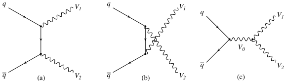
Figure 1: Leading-order Feynman diagrams for vector boson pair production. The assignments of $V_{0}$, $V_{1}$, and $V_{2}$ are: $V_{0}=V_{1}=W$ and $V_{2}=\gamma$ for $W\gamma$ production; $V_{0}=\gamma$ or $Z$, $V_{1}=W^{+}$ and $V_{2}=W^{-}$ for $WW$ production; $V_{0}=V_{1}=W$ and $V_{2}=Z$ for $WZ$ production; and $V_{0}=\gamma$ or $Z$, $V_{1}=Z$ and $V_{2}=\gamma$ for $Z\gamma$ production.

At leading order, associated production of gauge bosons takes place via the Feynman diagrams shown in Figure 1. The $W\gamma$ process has the highest cross section among the gauge boson pair production processes at the Tevatron. Many authors have discussed the use of $W\gamma$ production at hadron colliders to probe anomalous $WW\gamma$ couplings [49]. A tree level calculation of the $W\gamma$ cross section with anomalous couplings parametrized in the most general model-independent way, using the effective Lagrangian approach, has been performed by Baur and co-workers [50, 51].

In Figure 1a and 1b the $t$- and $u$-channel Feynman diagrams for $p\bar{p}\rightarrow\ell\nu\gamma$ correspond to photon bremsstrahlung from an initial-state quark. The $WW\gamma$ coupling appears in the $s$-channel process, Figure 1c. Events in which a photon is radiated from the final state lepton from single $W$ boson decay (Figure 2) also result in the same $\ell\nu\gamma$ final state.

The contributions from anomalous couplings to the helicity amplitudes for $p\bar{p}\rightarrow W\gamma$ can be written as [50]

$$\Delta{\cal M}_{\pm 0}={e^{2}\over{\rm sin}\,\theta_{W}}{\sqrt{\hat{s}}\over 2m_{W}}\left[\Delta\kappa_{\gamma}+\lambda_{\gamma}\mp i(\tilde{\kappa}_{\gamma}+\tilde{\lambda}_{\gamma})\right]{1\over 2}(1\mp{\rm cos}\,\Theta)$$

$$\Delta{\cal M}_{\pm\pm}={e^{2}\over{\rm sin}\,\theta_{W}}{1\over 2}\left[{\hat{s}\over m^{2}_{W}}(\lambda_{\gamma}\mp i\tilde{\lambda}_{\gamma})+(\Delta\kappa_{\gamma}\mp i\tilde{\kappa}_{\gamma})\right]{1\over\sqrt{2}}{\rm sin}\,\Theta,$$ (22)

where the subscripts of $\Delta{\cal M}$ denote the photon and $W$ helicities (the quark helicities are fixed by the $V-A$ structure of the $Wq\bar{q}$ coupling), and $\Theta$ denotes the scattering angle of the photon with respect to the quark direction, measured in the $W\gamma$ rest frame. From these expressions we see several important features:

(a) the cross section increases quadratically with the anomalous coupling parameters;

(b) due to the $\sqrt{\hat{s}}/m_{W}=\hat{\gamma}_{W}$ factors in these expressions, the effects of anomalies in the $WW\gamma$ vertex are enhanced at large parton subprocess energies. Therefore, a typical signature for anomalous couplings is a broad increase in the $W\gamma$ invariant mass at large values of $\hat{s}=m_{W\gamma}$;

(c) the sensitivity to $\lambda_{\gamma}$ will be higher than for $\Delta\kappa_{\gamma}$, because of the factor ${\hat{\gamma}_{W}}^{2}$ multiplying $\lambda_{\gamma}$ in Equation 22.

A striking feature of the $p\bar{p}\rightarrow W\gamma$ process is the prediction of radiation zeros in all the helicity amplitudes for SM $WW\gamma$ couplings. For $u\bar{d}\rightarrow W^{+}\gamma$ the amplitudes vanish at ${\rm cos}\,\Theta=-1/3$. In the presence of anomalous couplings the radiation zero is partially eliminated. This is evident from Equation 22 since all amplitudes are finite for nonzero anomalous couplings and ${\rm cos}\,\Theta=-1/3$. Consequently the average photon $p_{T}$ increases considerably in the presence of anomalous couplings and therefore the photon $p_{T}$ distribution is particularly sensitive to anomalous couplings. This effect, illustrated in Figure 3a, can be understood because anomalous couplings contribute through the $s$-channel diagram so their effects are evident predominantly in the central (low-rapidity) region. The photon $p_{T}$ is the quantity used in the DØ and CDF experiments to search for anomalous couplings because it is easier to measure than the $W\gamma$ invariant mass. The latter requires a knowledge of the neutrino longitudinal momentum, which cannot be measured at a $p\overline{p}$ collider.

The Feynman diagrams for $p\bar{p}\rightarrow Z\gamma$ are shown in Figure 1. Since the $Z$ has zero electric charge and zero weak isospin, the $ZZ\gamma$ and $Z\gamma\gamma$ couplings are zero at tree level in the SM, and the $s$-channel diagram only contributes in the presence of anomalous couplings. As a result there is no radiation zero in $Z\gamma$ production. Moreover, in the SM the ratio of the $Z\gamma$ cross section to the $W\gamma$ cross section rises with increasing minimum photon $p_{T}$ due to suppression of $W\gamma$ by the radiation zero, unlike the ratio for $Zj/Wj$, which is approximately independent of the minimum jet $p_{T}$ [54].

The leading-order helicity amplitudes and cross section for $Z\gamma$ production have been evaluated [53]. For anomalous couplings the $s$-channel diagram contributes, resulting in events with higher average photon $p_{T}$, as shown in Figure 3b. Defining $\hat{\gamma}_{Z}=\sqrt{\hat{s}}/m_{Z}$, it is found that the terms in the anomalous contributions to the helicity amplitudes are multiplied by factors of $\hat{\gamma}_{Z}^{3}$ for $h^{V}_{1}$ and $h^{V}_{3}$ and $\hat{\gamma}_{Z}^{4}$ for $h^{V}_{2}$ and $h^{V}_{4}$. Thus the growth with $\hat{s}$ is faster than for $W\gamma$ production and the experimental limits are more sensitive to the choice of form factor scale $\Lambda_{FF}$. Finally, we note that $Z\gamma$ production has been studied experimentally using the final states $\ell^{+}\ell^{-}\gamma$ and $\nu\bar{\nu}\gamma$. The latter has a higher branching fraction, and since there is no charged lepton involved, the final-state radiation process (as in Figure 2) is absent.

The $WW$ and $WZ$ production processes are also sensitive to anomalous couplings [55]. The $WW\gamma$ and $WWZ$ anomalous couplings enter via the $s$-channel diagram, Figure 1c. The effects are an increase in the average value of the invariant mass of the boson pair ($m_{WW}$ and $m_{WZ}$) and of the boson transverse momentum ($p_{T}^{W}$ and $p_{T}^{Z}$).

The $WW$ production process is sensitive to both the $WW\gamma$ and $WWZ$ couplings. When deriving limits on the anomalous couplings it is therefore customary to make assumptions about the relations between the $WW\gamma$ and $WWZ$ coupling parameters in order to reduce the number of free parameters. For example, one can assume SM $WW\gamma$ couplings and derive limits on the $WWZ$ coupling parameters or vice versa. The sensitivity to the $WWZ$ couplings is higher due to the overall coupling $g_{WWZ}$ for the $WWZ$ vertex, which is larger than the corresponding factor $g_{WW\gamma}$ for the $WW\gamma$ vertex. Alternatively, one can assume equal $WWZ$ and $WW\gamma$ couplings ($\Delta\kappa_{\gamma}=\Delta\kappa_{Z}$, etc), or use the HISZ assumption (see Section 1.1.1). The $WZ$ production process has the advantage of being sensitive only to the $WWZ$ coupling, but it has a smaller cross section. The SM cross sections are $\sigma_{WW}=9.5$ pb [57] and $\sigma_{WZ}=2.5$ pb [58] at next-to-leading order.

An important consideration for the experimental study of diboson production at the Tevatron is the effects of higher order c on the cross sections and kinematic distributions. Next-to-leading–order calculations have been performed for SM and anomalous couplings for $W\gamma$ [56, 59], $Z\gamma$ [52], $WW$ [57, 60], and $WZ$ [58, 61] production at hadron colliders. At the Tevatron energy, the next-to-leading–order cross sections are generally a factor of $\sim 30$% higher than the leading-order calculations. The shapes of the kinematic distributions are, to a good approximation, unchanged compared with leading order. Therefore, the analyses described below have used leading-order Monte Carlo event generators with a K-factor of $1+\frac{8}{9}\pi\alpha_{s}(M_{W}^{2})\approx 1.34$ to approximate the effects of the QCD corrections. The transverse momentum of the diboson system is modeled based on the observed $W$ $p_{T}$ spectrum in inclusive $W\rightarrow e\nu$ events.

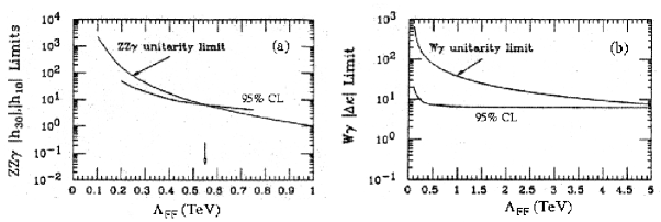
Figure 4: Experimental 95% confidence level limits and unitarity limits as a function of form factor scale $\Lambda_{FF}$ for (a) the $ZZ\gamma$ coupling $h^{Z}_{30}$ and (b) the $WW\gamma$ coupling $\Delta\kappa$ [from  [63]]. Note that the experimental limits have been superseded by the much tighter limits described in Section 5.

Experimental limits on the anomalous couplings are derived using the form factor ansatz described in Section 1.1.3. The motivation for the choice of the form factor scale $\Lambda_{FF}$ is illustrated in Figure 4a, which shows an old experimental limit and the corresponding unitarity limit [62] as a function of $\Lambda_{FF}$ for the $ZZ\gamma$ coupling parameter $h^{Z}_{30}$. At large $\Lambda_{FF}$ the unitarity limit becomes more stringent than the experimental limit. Therefore, $\Lambda_{FF}$ is chosen to be as large as possible consistent with unitarity as indicated by the vertical arrow in Figure 4a. In practice, round numbers (e.g. $\Lambda_{FF}=500$ GeV) are used to allow easy comparison of results between different experiments. For $W\gamma$ production, the limits depend only weakly on the form factor scale for $\Lambda_{FF}$ above about 500 GeV, as shown in Figure 4b.

3 THE TEVATRON COLLIDER AND DETECTORS

3.1 The Tevatron Proton–Antiproton Collider

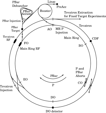
Figure 5: The Fermilab accelerator complex, from Ref. [64].

A schematic of the Fermilab accelerator complex [64] is shown in Figure 5. In the Linac, 18 keV $H^{-}$ ions from a Cockroft-Walton electrostatic generator are accelerated to an energy of 200 MeV. The electrons are then stripped off and the remaining protons are injected into the Booster, where they are accelerated to 8 GeV. They are then transferred to the Main Ring, a 1 km–radius synchrotron located in the same tunnel as the Tevatron. Protons are accelerated to 150 GeV in the Main Ring and injected into the Tevatron. The Tevatron [65] was the first large accelerator to use superconducting magnets for the main guide field. It accelerates protons and antiprotons to a final energy of 900 GeV.

The Main Ring also provides a beam of 120 GeV protons, which are extracted and strike a target, producing antiprotons with a peak energy of 8 GeV [66]. The antiprotons are stochastically cooled and stacked in the Debuncher and Accumulator and transferred to the Main Ring for injection into the Tevatron.

One of the main limitations on the achievable luminosity is the number of antiprotons in the accelerator. During Run I (1992–1996), the Tevatron was operated with six antiproton (and six proton) bunches and with $\approx$$7\times 10^{10}$ antiprotons per bunch. This led to peak luminosities of $\approx$$3\times 10^{31}$ cm^-2 s^-1. The time interval between bunches, which determined the interval between collisions in each detector, was 3.5 $\mu$s during Run I.

3.2 The CDF and DØ Detectors

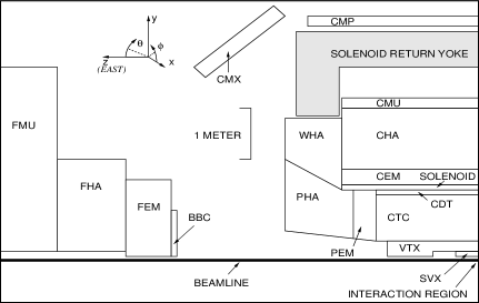
Figure 6: A cross-sectional side view of the CDF detector [from [70]]. SVX, VTX, CTC, and CDT are tracking detectors. The calorimeters are CEM, CHA, WHA, PEM, PHA, FEM, and FHA. The muon detectors are CMU, CMP, CMX, and FMU.

The CDF detector [67] is shown in Figure 6. The tracking system consists of an inner silicon microstrip vertex detector, a set of time projection chambers, and an outer central tracking chamber, covering $|\eta|<1.1$. The pseudorapidity $\eta$ is defined as $\eta=-{\rm ln}\left[{\rm tan}\,\theta/2\right]$, where $\theta$ is the polar angle with respect to the beam axis.

These detectors provide a measurement of the transverse momentum $p_{T}$ of charged particles with a resolution of $\sigma(p_{T})/p_{T}\approx$ $\sqrt{(0.9p_{T})^{2}+(6.6)^{2}}\times 10^{-3}$, where $p_{T}$ is in GeV/$c$. The central electromagnetic and hadronic calorimeters consist of lead-scintillator and steel-scintillator sampling detectors, respectively. The energy resolution for $|\eta|<1.1$ is $\sigma(E)/E$ $\approx$14%$/\sqrt{E}$ for electrons and $\approx$(50 to 75)%$/\sqrt{E}$ for isolated pions where $E$ is in GeV. In the forward region ($1.1<|\eta|<4.2$) the calorimeters use proportional chambers and have energy resolution $\approx$25%$/\sqrt{E}$ for electrons and $\approx$110%$/\sqrt{E}$ for isolated pions. The calorimeter projective tower segmentation in the central region is $0.1\times 0.26$ in $\eta\times\phi$, where $\phi$ is the azimuthal angle, while in the forward region it is $0.1\times 0.09$. The central muon system consists of a set of drift chambers and steel absorbers covering the region $|\eta|<1.0$.

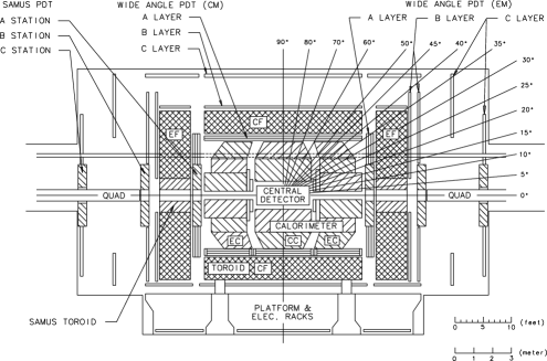
Figure 7: Cross-sectional side view of the DØ detector [from [68]], showing the central detector, the calorimeters (CC, EC), and the muon system (CF, EF, SAMUS, and proportional drift chambers (PDTs).

The DØ detector [68] consists of three main systems (Figure 7). The central drift chamber and forward drift chambers are used to identify charged tracks for $|\eta|<3.2$ and to measure the position of interaction vertices along the direction of the beam. The calorimeter consists of uranium/liquid-argon sampling detectors with fine segmentation, and is divided into a central and two endcap cryostats covering $|\eta|<4.4$. The energy resolution of the calorimeter is $\approx$15%$/\sqrt{E}$ for electrons and $\approx$50%$/\sqrt{E}$ for isolated pions. The calorimeter towers subtend $0.1\times 0.1$ in $\eta\times\phi$, segmented longitudinally into four electromagnetic (EM) layers and four or five hadronic layers. In the third EM layer, at the EM shower maximum, the cells are $0.05\times 0.05$ in $\eta\times\phi$. The muon system consists of magnetized iron toroids with one inner and two outer layers of drift tubes, providing coverage for $|\eta|<3.3$.

4 DETECTION OF ASSOCIATED GAUGE BOSON
PRODUCTION

In the Tevatron Run I analyses of diboson events, the following final states are considered:

1. $W\gamma\rightarrow\ell\nu\gamma$
           2. $WW\rightarrow\ell\nu~{}\ell\nu$
           3. $WW/WZ\rightarrow\ell\nu~{}q\bar{q}$
           4. $WZ\rightarrow q\bar{q}~{}\ell^{+}\ell^{-}$
           5. $Z\gamma\rightarrow\ell^{+}\ell^{-}\gamma$
           6. $Z\gamma\rightarrow\nu\bar{\nu}\gamma$

where $\ell=e$ or $\mu$. Except for $Z\gamma\rightarrow\nu\bar{\nu}\gamma$, only electron and muon decays of the $W$ and $Z$ have been studied, as they provide a unique experimental signature of high-$p_{T}$ isolated leptons. Although CDF have reported a $WZ\rightarrow e\nu~{}ee$ candidate event and a $ZZ\rightarrow\mu\mu~{}\mu\mu$ candidate event in their data [69], these modes have not been studied so far due to the much lower cross section times branching fraction (less than one event is expected in each mode in Run I). Detection of charged leptons, neutrinos, photons, and jets from the six processes listed above is discussed in the following sections.

4.1 Detection of Leptonic W and Z Decays

Electrons from $W$ or $Z$ decays are identified as tracks in the tracking chambers pointing to the centroid of a shower in the electromagnetic calorimeters. To discriminate against charged hadrons, the profile of energy deposition in the calorimeter and the fraction of electromagnetic energy to hadronic energy must be consistent with electron test beam studies and with clean samples of electrons obtained from collider data. The electron calorimeter showers are required to be isolated from nearby energy deposition in the calorimeter. CDF also use track isolation.

Muons are reconstructed as tracks in the muon chambers. Additional identification requirements are used to reject cosmic ray muons and hadrons, which interact in the calorimeters. The impact parameter of the muon track from the beamline and from the interaction vertex $z$-position must be consistent with that of a particle originating from the hard collision, and the energy deposited in the calorimeters must be characteristic of a minimum ionizing particle. In DØ the muon must also be coincident with the beam crossing time. In CDF the muon transverse momentum is measured using the central tracking chamber; in DØ it is measured using the muon chambers and toroidal field with a resolution of $\sigma(1/p)\approx 0.18(p-2)/p^{2}\oplus 0.008$, with $p$ in GeV/$c$. Therefore, the CDF measurement of momentum is more precise. The muon tracks are required to be isolated from nearby jets and from energy deposition in the calorimeters. CDF also uses track isolation in the central tracking chambers.

Neutrinos from $W$ decays are inferred from the missing transverse energy in an event. The neutrino $p_{T}$ is calculated from the missing energy in the calorimeters and the transverse momentum of muons in the event (if any).

4.2 Photon Detection

Photons must satisfy the same selection criteria as electrons, except that the electromagnetic shower must not be accompanied by a matching track. In some of the DØ analyses, photon candidates containing hits in the region of the central tracking chambers between the interaction vertex and the EM cluster centroid are rejected too, as this indicates an unreconstructed track.

In the $W\gamma$ and $Z\gamma$ analyses, an important source of background originates from $W$ + jet and $Z$ + jet events, where jet fragmentation fluctuations lead to a single neutral meson such as a $\pi^{0}$ carrying most of the energy of the jet. For meson transverse energies above about 10 GeV, the showers from the two decay photons coalesce and mimic a single photon shower in the calorimeter.

To estimate these backgrounds it is necessary to calculate the probability that a jet “fakes” a photon, $P(j\rightarrow``\gamma$”). In both DØ and CDF this is done using a sample of multijet events obtained from jet triggers, which are independent of the triggers used to select the $W\gamma$ and $Z\gamma$ signal events. The probability is determined as a function of the $E_{T}$ of the jet by measuring the fraction of nonleading jets in the multijet sample that passes the photon identification requirements. To avoid trigger biases associated with the calorimeter energy response at trigger threshold, only the nonleading jets are used, i.e. those jets that did not fire the trigger.

The multijet samples also contained genuine direct photons, predominantly from gluon Compton scattering. In DØ the fraction of such direct photons in the sample is determined using the energy deposited in the first layer of the EM calorimeter. Since meson decays produce two photons, which can independently convert to an $e^{+}e^{-}$ pair in the calorimeter, showers originating from mesons start earlier than single photon showers and produce more energy in the first layer of the calorimeter. In CDF the transverse shape of the shower at the shower maximum is used, since on average it is broader for meson decay showers than for single photon showers. The resulting probability $P(j\rightarrow``\gamma$”) is found to be in the range $\approx 10^{-4}-10^{-3}$, depending on the photon identification requirements and on $E_{T}$.

4.3 Jet Detection

In the processes $WW/WZ\rightarrow\ell\nu~{}q\bar{q}$ and $WZ\rightarrow q\bar{q}~{}\ell^{+}\ell^{-}$, either a $W$ or a $Z$ decays to a $q\bar{q}$ pair, which hadronizes to form jets. Production of single $W$ or $Z$ bosons with a subsequent decay to two jets has not been observed at the Tevatron due to the overwhelming background from two-jet events. In the region of the $W$ and $Z$ masses, this background consists mainly of gluon jets, which are indistinguishable from quark jets on an event-by-event basis.

Similarly, $WW$ and $WZ$ production in which one boson decays to leptons and the other to a $q\bar{q}$ pair has not been isolated from the very large background due to $W\,+\,jj$ or $Z\,+\,jj$ production and multijet production. However, to retain good acceptance for the SM signal and anomalous $WW$ and $WZ$ production while minimizing the backgrounds, the analyses require events to contain two jets that form an invariant mass consistent with the $W$ or $Z$ mass. The jet energy resolutions are typically $\sigma(E)/E\approx$100%$/\sqrt{E}$ with $E$ in GeV. The dijet invariant mass resolution is approximately 10 GeV$/c^{2}$ for $m_{jj}=80$ GeV$/c^{2}$.

Jets are detected in the CDF and DØ hadron calorimeters using a fixed cone clustering algorithm with cone radius $R=\sqrt{\Delta\eta^{2}+\Delta\phi^{2}}$. For the analyses under consideration here, cone sizes of $R=0.3,0.4$, and 0.5 have been used. For smaller cone sizes, fragmentation effects cause particles to be lost outside the clustering cone, resulting in poorer energy resolution. For larger cone sizes, more energy associated with the underlying event is included within the cone, also resulting in poorer energy resolution; furthermore, jets close together in $\eta-\phi$ space tend to be merged into one jet. The latter effect results in low efficiency for detecting the $W\rightarrow q\bar{q}$ and $Z\rightarrow q\bar{q}$ decays, especially at high boson transverse momentum, since the opening angle of the two jets decreases as the $p_{T}$ of the boson rises. Typically, the efficiency starts to drop off for $p_{T}(jj)>$ 200 to 300 GeV$/c$.

5 ANALYSIS AND RESULTS

5.1 $W\gamma$ Analysis Results

The published results on $W\gamma$ production at the Tevatron are from the CDF analysis of data from Run Ia [71, 63] (1992–1993) and the DØ analyses of data from Runs Ia and Ib [72, 73, 74] (1994–1995). Also described in this section are the preliminary results from the CDF analysis of data from Run Ib [75].

In the analyses, a high $p_{T}$ electron or muon is required (see Table 3), accompanied by large missing transverse energy, indicating the presence of a $W$ boson. A high $p_{T}$ isolated photon is also required, with $p_{T}>7$ GeV$/c$ for CDF and $p_{T}>10$ GeV$/c$ for DØ. The higher $p_{T}$ cut used by DØ results in a lower acceptance, but does not reduce the sensitivity to anomalous couplings, because anomalous couplings would result in events with higher $p_{T}$ photons compared with the SM. The photon is required to be separated from the lepton by $\Delta R_{\ell\gamma}>0.7$ units in $\eta-\phi$ space, which reduces the background from radiative $W$ decays. Photons and electrons are detected in the pseudorapidity range $|\eta|<1.1$ for CDF and $|\eta|<1.1$ or $1.5<|\eta|<2.5$ for DØ. This results in a higher geometrical acceptance for DØ.

The backgrounds are from the following sources: (a) $W$ + jet production, where the jet fluctuates to a neutral meson such as a $\pi^{0}$ which decays to two photons; (b) $Z\gamma$ events in which one of the leptons from the $Z$ decay is not reconstructed; (c) $W(\tau\nu)\gamma$ production with the decay $\tau\rightarrow\ell\nu\nu$; and (d) processes (labeled $\ell eX$) that produce missing transverse energy, a high-$p_{T}$ lepton, and an electron with an unreconstructed track. The dominant background is from (a). This background is estimated from the observed $E_{T}$ spectrum of jets in the inclusive $W\rightarrow\ell\nu$ data samples and from the measured probability for a jet to fake a photon (see Section 4.2). The smaller backgrounds from (b) and (c) are estimated using Monte Carlo simulations. Background (d) is significant only in the DØ analysis due to the small but nonzero inefficiency for reconstructing tracks associated with electrons. The sources of this background are from $t\bar{t}$ and $WW$ pair production with a subsequent $W\rightarrow\ell\nu$ decay, and in the electron channel, high-$p_{T}$ $Z\rightarrow ee$ and multijet production.

Theoretical predictions of $W\gamma$ production are made based on the leading-order Monte Carlo program of Baur & Zeppenfeld [50, 51] (see Section 2). The efficiencies and acceptances of the CDF and DØ detectors are modeled using fast Monte Carlo programs that include geometrical acceptances and smearing effects due to detector resolutions.

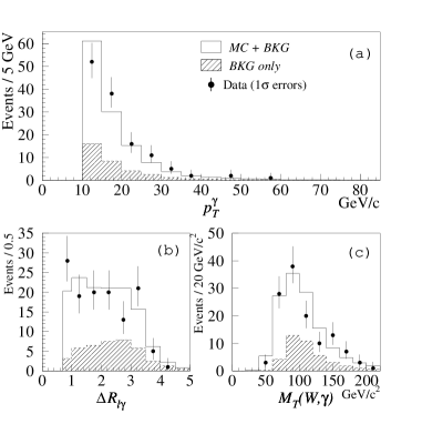
Figure 8: Distributions of (a) photon transverse energy $p_{T}^{\gamma}$, (b) lepton-photon separation $\Delta R_{\ell\gamma}$, and (c) transverse cluster mass $M_{T}(W,\gamma)$ for the DØ $W\gamma$ analysis.

Table 4 compares the numbers of signal events after background subtraction with the SM predictions. The number of events is of the order of 100 for each experiment. The DØ measured cross section times branching fraction (with $E_{T}^{\gamma}>10~{}{\mathrm{Ge\kern-1.00006ptV}}$ and $\Delta R_{\ell\gamma}>0.7)$ is $\sigma(W\gamma)\times B(W~{}\rightarrow~{}\ell\nu)=11.3^{+1.7}_{-1.5}~{}{\rm(stat)}\pm 1.5$ (syst) pb compared with the SM prediction of $\sigma(W\gamma)\times B(W\rightarrow\ell\nu)=12.5\pm 1.0$ pb. Figure 8 shows the DØ $p_{T}^{\gamma}$ distribution for the observed candidate events together with the SM signal prediction plus the sum of the estimated backgrounds. The number of observed events and the shapes of the distributions show no deviations from the expectations.

In both experiments, limits on the $WW\gamma$ vertex coupling parameters are obtained from a binned maximum likelihood fit to the photon $p_{T}$ distribution. The likelihood function is given by

$$P(\sigma|n) = \int_{0}^{\infty}d{s_{i}}\int_{0}^{\infty}d{b_{i}}\prod_{i}\frac{e^{-(b_{i}+s_{i})}(b_{i}+s_{i})^{n_{i}}}{n_{i}!}$$ (23)

$$\times G(s_{i};s_{i0},\sigma_{s_{i}})G(b_{i};b_{i0},\sigma_{b_{i}}),$$

where $b_{i}+s_{i}$ is the predicted number of events in the $i^{\rm th}$ bin, $b_{i}$ is the estimated background in the $i^{\rm th}$ bin, $s_{i}={\cal L}\epsilon_{i}\sigma_{i}$ is the predicted number of signal events in the $i^{\rm th}$ bin, ${\cal L}$ is the integrated luminosity, $\epsilon_{i}$ is the efficiency for the $i^{\rm th}$ bin, $\sigma_{i}$ is the $W\gamma$ cross section prediction for the $i^{\rm th}$ bin, and $n_{i}$ is the observed number of events in the $i^{\rm th}$ bin. In the above expression, the Poisson probability for each bin is convolved with two Gaussian distributions $G$, which represent the uncertainties in the background estimate and the predicted number of signal events. This method [76] incorporates these uncertainties into the confidence interval calculation using a Bayesian statistical approach, while the Poisson probability is treated classically. The quantity $s_{i}=s_{i}(\Delta\kappa_{\gamma},\lambda_{\gamma})$ depends on the anomalous coupling parameters $\Delta\kappa$ and $\lambda$. To exploit the fact that anomalous coupling contributions lead to an excess of events at high photon $p_{T}$, a high $p_{T}$ bin in which no events were observed is explicitly included in the histogram. The nonobservation of events in this bin carries information on the anomalous couplings [77].

For the $W\gamma$ analysis and the analyses described in subsequent sections, the uncertainties are typically $\approx$10% from the errors in the measured detection efficiencies, $\approx$5% from the choice of parton distribution function (pdf), $\approx$1% from varying the $Q^{2}$ at which the pdf’s are evaluated, $\approx$5% from the modeling of the diboson transverse momentum, and $\approx$6% from the integrated luminosity measurement error. The uncertainty in the background estimates varies from 12% to 30% depending on the particular analysis channel.

In the electron channel Run Ib analysis, DØ requires the electron-photon-neutrino transverse cluster mass to be $>90$ GeV$/c^{2}$. This requirement suppresses radiative $W$ decays and increases the sensitivity to anomalous couplings by about 10%. Figure 9 shows the 95% confidence level (CL) limits in the $\Delta\kappa_{\gamma}-\lambda_{\gamma}$ plane, for a form factor scale of $\Lambda_{FF}=1.5~{}{\mathrm{Te\kern-1.00006ptV}}$. Varying only one coupling at a time from its SM value, the following limits are obtained at the 95% CL:

DØ:	$-0.93<\Delta\kappa_{\gamma}<0.94$
	$-0.31<\lambda_{\gamma}<0.29$
CDF:	$-1.8<\Delta\kappa_{\gamma}<2.0$
	$-0.70<\lambda_{\gamma}<0.60$

The possibility of a minimal U(1)_EM-only coupling ($\kappa=\lambda=0$) indicated by the solid circle in Figure 9 is ruled out at the 88% CL by the DØ measurement. Figure 10 shows the limits on a plot of $W$ boson electric quadrupole moment $Q_{W}$ vs magnetic dipole moment $\mu_{W}$.

The ${\rm cos}\,\Theta$ distribution in the data is consistent with the SM prediction [75], where $\Theta$ is the scattering angle of the photon with respect to the quark direction, measured in the $W\gamma$ rest frame. However, at present the integrated luminosity is too low to establish the presence of the radiation zero.

5.2 $WW\rightarrow\ell\nu\ell^{\prime}\nu^{\prime}$ Analysis Results

The CDF and DØ experiments have searched for $W^{+}W^{-}$ production in the dilepton decay modes $e\nu e\nu$, $e\nu\mu\nu$, and $\mu\nu\mu\nu$ [79, 80, 81]. The event selection requirements are summarized in Table 5. The CDF and DØ analyses each require two isolated leptons plus missing transverse energy, using similar selection criteria.

Background from top quark pair production ($p\bar{p}\rightarrow t\bar{t}+X\rightarrow W^{+}W^{-}b\bar{b}+X$) is suppressed by removing events that contain hadronic energy in the calorimeters. DØ requires the vector sum of the $E_{T}$ from hadrons ${\vec{E}}_{T}^{\rm had}$, defined as ${\vec{E}}_{T}^{\rm had}=-({\vec{E}}_{T}^{\ell 1}+{\vec{E}}_{T}^{\ell 2}~{}+~{}$${\hbox{${\vec{E}}$\kern-6.00006pt\lower-0.43057pt\hbox{/}}}_{T}$$)$, to be less than 40 GeV. For $W^{+}W^{-}$ events, gluon radiation and detector resolution give rise to small values of ${\vec{E}}_{T}^{\rm had}$ compared with $t\bar{t}$ events, where the main contribution is from the $b$-quark jets from the $t$-quark decays. This cut reduces the background from $t\bar{t}$ production by a factor of more than four for $m_{t}=170$ GeV$/c^{2}$, with an efficiency of 95% for SM $W^{+}W^{-}$ events. CDF suppresses the $t\bar{t}$ background by removing events containing any jet with $E_{T}>10$ GeV.

To discriminate against backgrounds from $Z\rightarrow\tau^{+}\tau^{-}$ and the Drell-Yan processes $\gamma/Z\rightarrow e^{+}e^{-},\mu^{+}\mu^{-}$, a ${\hbox{$E$\kern-6.00006pt\lower-0.43057pt\hbox{/}}}_{T}$ cut is applied (Table 5). Events are also rejected if the ${\hbox{$E$\kern-6.00006pt\lower-0.43057pt\hbox{/}}}_{T}$ vector points along the direction of a lepton or opposite to the direction of a lepton (within $20^{\circ}$) and the ${\hbox{$E$\kern-6.00006pt\lower-0.43057pt\hbox{/}}}_{T}$ is less than 50 GeV. Finally, events with a dilepton mass within the limits 75 GeV$/c^{2}<m_{\ell^{+}\ell^{-}}<105$ GeV$/c^{2}$ are rejected.

In the DØ analysis based on an integrated luminosity of 97 pb^-1, five events pass the event selection criteria and the total estimated background is $3.1\pm 0.4$ events. This leads to an upper limit on the cross section for $p\bar{p}\rightarrow W^{+}W^{-}$ of 37.1 pb at the 95% CL.

In the CDF analysis based on 108 pb^-1 of data, the event selection also yields five events, but with an estimated background of only $1.2\pm 0.3$ events. The probability that the observed events correspond to a fluctuation of the background is 1.1%. The $W^{+}W^{-}$ cross section is measured to be $\sigma(p\bar{p}\rightarrow W^{+}W^{-})=10.2^{+6.3}_{-5.1}\pm 1.6$ pb. This is in good agreement with the next-to-leading–order cross section for SM $W$ pair production calculated by Ohnemus [57], which gives the result $\sigma_{SM}(p\bar{p}\rightarrow W^{+}W^{-})=9.5$ pb. Because of the higher signal-to-background ratio, CDF is able to make a measurement of the cross section rather than set an upper limit as DØ does.

The $W$ pair production process is sensitive to both the $WW\gamma$ and $WWZ$ couplings, since the $s$-channel propagator can be a $\gamma$ or a $Z$. Anomalous couplings result in a higher cross section and an enhancement of events with high $p_{T}$ $W$ bosons. In the CDF analysis the total cross section is used in setting limits, while in the DØ analysis a binned maximum likelihood fit is performed to the measured $p_{T}$ spectra of the two leptons in each event [81]. This technique is similar to that described for the $W\gamma$ analysis previously. However, there is a correlation between the $p_{T}$ of one lepton and the $p_{T}$ of the other lepton in the same event because the two $W$ bosons are boosted by approximately the same amount in opposite directions (${\vec{p}}_{T}^{W^{+}}\approx-{\vec{p}}_{T}^{W^{-}}$). This correlation is stronger for larger anomalous couplings because of the higher $p_{T}$ of the $W$ bosons in these events. To account for this correlation, two-dimensional bins in the $p_{T}$ of one lepton vs the $p_{T}$ of the other lepton are used. Use of this kinematic information provides significantly tighter constraints on anomalous couplings than those obtained from the measurement of the cross section alone. Both experiments use a tree-level Monte Carlo program [55] to generate $W^{+}W^{-}\rightarrow\ell^{+}\nu\ell^{-}\bar{\nu}$ events as a function of the coupling parameters.

Varting only one coupling at a time and assuming $\Delta\kappa_{Z}=\Delta\kappa_{\gamma}$ and $\lambda_{Z}=\lambda_{\gamma}$, the DØ results based on 97 pb^-1 of data using the kinematic likelihood fit method yield the following 95% CL limits for a form factor scale of $\Lambda_{FF}=1.5$ TeV:

$-0.62<\Delta\kappa<0.77$

$-0.52<\lambda<0.56$.

The limits obtained by CDF using the cross section alone are slightly looser than the DØ limits and are given in reference [80].

5.3 $WW/WZ\rightarrow\ell\nu jj$ and $WZ\rightarrow jj\ell\ell$ Analysis Results

In the lepton-plus-jets analyses CDF [82, 69] and DØ [83, 84] search for candidate $WW/WZ\rightarrow\ell\nu jj$ events containing a high $p_{T}$ lepton, missing $E_{T}$  and two jets with invariant mass consistent with the $W$ or $Z$ mass (taking into account the dijet mass resolution of $\approx 10$ GeV$/c^{2}$). The event selection requirements are given in Table 6. CDF also accepts events with two charged leptons and two jets resulting from $p\bar{p}\rightarrow WZ\rightarrow jj\ell^{+}\ell^{-}$. The event selection is similar in all respects, except that a second lepton is required in place of the missing $E_{T}$ requirement. CDF has analyzed the electron and muon decay channels, while DØ has so far only analyzed the $e\nu jj$ final state.

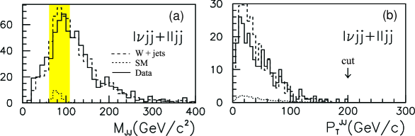
Figure 11: CDF selection of $W/WZ\rightarrow\ell\nu jj,\ell\ell jj$ events. (a) Dijet mass distribution for events passing all selection requirements except the dijet mass cut. (b) The $p_{T}$ of the two-jet system for the subset of events from (a) passing the dijet mass cut [shaded region in (a)]. The distributions are shown for the data (solid line), the $W+$ jets background (dashed line), and the SM prediction (dotted line).

The CDF and DØ analyses follow similar lines. After applying the lepton, missing $E_{T}$  and jet requirements, the invariant mass of the dijet system is histogrammed. For events containing more than two jets, CDF takes the two leading jets whereas DØ uses the dijet combination with the largest invariant mass. Figure 11a shows the resulting histogram for the CDF Run Ib preliminary analysis. The dijet mass cut (see Table 6), which selects the events falling within the shaded band in the figure, is then applied. The transverse momentum of the two-jet system for this subset of events is shown in Figure 11b.

Jet cone radii of $R=0.3,0.4$, and 0.5 were used in the analyses (see Table 6). We discuss the motivations for these choices in Section 4.3

As shown in Figure 11, the data are dominated by background, mainly from $W~{}+\geq 2$ jets events with $W\rightarrow e\nu$ and (in DØ) multijet production where one jet is misidentified as an electron and there is significant (mismeasured) missing $E_{T}$. However, at large values of $p_{T}^{W}$ the backgrounds are relatively small and it is predominantly in this region where anomalous couplings enhance the cross section. This is the key to obtaining limits on the anomalous couplings. The main difference between the analyses is that CDF applies a cut on the boson transverse momentum ($p_{T}^{W}=p_{T}^{jj}>200$ GeV$/c$) and extracts limits on the anomalous couplings from the number of events surviving the cut, whereas DØ uses a binned likelihood fit to the $W$ boson $p_{T}$ spectrum. The latter technique is analogous to the fit to the $p_{T}^{\gamma}$ distribution in the $W\gamma$ analysis.

The CDF analysis estimates the backgrounds from $W~{}+\geq 2$ jets and $Z~{}+\geq 2$ jets using the vecbos [85] event generator followed by parton fragmentation using the herwig [86] package and a Monte Carlo simulation of the CDF detector. The boson $p_{T}$ requirement for $WW$ and $WZ$ event selection is chosen so that less than one background event is expected in the final sample. Therefore, no background subtraction is necessary and theoretical uncertainties in the background calculation are avoided. Because no background subtraction is made, conservative limits on anomalous couplings are obtained. In DØ the $W~{}+\geq 2$ jets background is estimated with vecbos, herwig  and a geant [87] simulation of the DØ detector. The $W~{}+\geq 2$ jets background is normalized by comparing the number of events expected from the vecbos estimate to the number of candidate events observed in the data outside the dijet mass window, after the multijet background has been subtracted. Using this method the systematic uncertainties in this background are due only to the normalization and the jet energy scale uncertainty.

The data are in good agreement with the expected backgrounds plus SM signal for both analyses. No excess of events at large $p_{T}^{W}$ is observed and the overall shape of the $p_{T}^{W}$ distribution agrees well with the predictions. Limits are derived using the leading-order calculation by Hagiwara et al [55] to obtain the expected $WW$ and $WZ$ signal as a function of the anomalous couplings.

Varying only one coupling at a time and assuming equal $WW\gamma$ and $WWZ$ couplings, the 95% CL limits obtained from DØ and CDF are, for $\Lambda_{FF}=2$ TeV, as follows:

DØ:	$-0.43<\Delta\kappa<0.59$
	$-0.33<\lambda<0.36$
CDF:	$-0.49<\Delta\kappa<0.54$
	$-0.35<\lambda<0.32$.

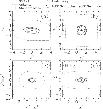
Figure 12: Allowed regions for anomalous couplings from the preliminary CDF analysis. All couplings, other than those plotted for each contour, are held at their SM values: (a) $\lambda_{Z}$ vs $\lambda_{\gamma}$; (b) $\kappa_{Z}$ vs. $g_{1}^{Z}$; (c) $\lambda$ vs $\kappa$ assuming the $WWZ$ and $WW\gamma$ coupling parameters are equal; and (d) limits on the couplings $\kappa_{\gamma}$, $\kappa_{Z}$, $\lambda_{\gamma}$, $\lambda_{Z}$, and $g_{1}^{Z}$ in the HISZ scenario with independent variables $\kappa_{\gamma}$ and $\lambda_{\gamma}$.

Figure 12 shows the limits obtained in the CDF analysis. Figure 12a shows limits in the $\lambda_{\gamma}-\lambda_{z}$ plane with all other couplings held at their SM value. The limits are stronger for $\lambda_{z}$, illustrating the fact that this analysis is in general more sensitive to the $WWZ$ coupling parameters (see Section 2).

The limits of Figure 12b focus on the $WWZ$ vertex, assuming that the $WW\gamma$ couplings take the SM values. The point $\kappa_{Z}=\lambda_{Z}=0$ representing the minimal U(1)_EM-only coupling (corresponding to zero $WWZ$ coupling) lies outside the allowed region and is excluded at the 99% CL by both experiments. This is the first direct evidence for the existence of the $WWZ$ coupling, and for the destructive interference between the $s$-channel and $t$- or $u$-channel diagrams which takes place in the SM.

In Figure 12c the $WWZ$ and $WW\gamma$ coupling parameters are assumed to be equal ($\kappa_{Z}=\kappa_{\gamma}$, $\lambda_{Z}=\lambda_{\gamma}$), while in Figure 12d the HISZ relations are assumed.

5.4 DØ Combined Analysis of $WW\gamma$ and $WWZ$ Couplings

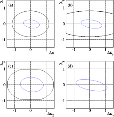
Figure 13: DØ limits on anomalous couplings for $\Lambda_{FF}=1.5$ TeV from a simultaneous fit to the $W\gamma$, $WW\rightarrow\ell\nu\ell^{\prime}\nu^{\prime}$, and $WW/WZ\rightarrow e\nu jj$ data: (a) assuming $\Delta\kappa_{Z}=\Delta\kappa_{\gamma}$, $\lambda_{Z}=\lambda_{\gamma}$; (b) assuming the HISZ scenario; (c) assuming SM $WW\gamma$ couplings; and (d) assuming SM $WWZ$ couplings. The inner curves are the 95% CL limits and the outer curves are the unitarity limits. In (d) the unitarity limits lie outside the boundary of the plot.

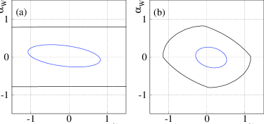
Figure 14: DØ limits on anomalous couplings for $\Lambda_{FF}=1.5$ TeV from a simultaneous fit to the $W\gamma$, $WW\rightarrow\ell\nu\ell^{\prime}\nu^{\prime}$, and $WW/WZ\rightarrow e\nu jj$ data for: (a) $\alpha_{W}$ vs $\alpha_{B\phi}$ when $\alpha_{W\phi}=0$; and (b) $\alpha_{W}$ vs. $\alpha_{W\phi}$ when $\alpha_{B\phi}=0$. The inner curves are the 95% CL limits and the outer curves are the unitarity limits.

DØ has performed a simultaneous fit to the photon $p_{T}$ distribution in the $W\gamma$ data, the lepton $p_{T}$ distribution in the $WW\rightarrow\ell\nu\ell^{\prime}\nu^{\prime}$ data, and the $p_{T}^{e\nu}$ distribution in the $WW/WZ\rightarrow e\nu jj$ data [81]. Limits on the $WW\gamma$ and $WWZ$ coupling parameters are extracted from the fit, taking care to account for correlations between the uncertainties on the integrated luminosity, the selection efficiencies, and the background estimates. The fit is performed using the parameters $\Delta\kappa,\lambda$, and $g_{1}^{Z}$ and also using the set $\alpha_{B\phi},\alpha_{W\phi}$, and $\alpha_{W}$. The results are given in Figures 13 and 14 and Tables 7 and 8. These are the most stringent limits to date on the $WW\gamma$ and $WWZ$ coupling parameters $\Delta\kappa$, $\lambda$, and $\Delta g_{1}^{Z}$.

The DØ limits also provide the most stringent constraints on the parameters $\alpha_{B\phi}$ and $\alpha_{W}$. The LEP measurements are more sensitive to $\alpha_{W\phi}$ than to $\alpha_{B\phi}$ and $\alpha_{W}$. The LEP limits are complimentary to the Tevatron limits because they are obtained from a different process (i.e. $e^{+}e^{-}\rightarrow W^{+}W^{-}$) using angular distributions of the decay products.

5.5 $Z\gamma$ Analysis Results

5.5.1 $p\bar{p}\rightarrow\ell^{+}\ell^{-}\gamma+X$

This subsection describes the search for $Z\gamma$ events in which the $Z$ decays to $e^{+}e^{-}$ or $\mu^{+}\mu^{-}$. The event selection requirements are similar to those for the $W\gamma$ analysis except that instead of the missing transverse energy requirement, a second charged lepton is required with looser particle identification criteria. The photon selection requirements are almost identical to those used in the $W\gamma$ analyses as listed in Table 3. The CDF analyses [63, 75, 89] and the DØ analyses [73, 90, 91] are described elsewhere.

The main source of background is from $Z~{}+$ jet production where the jet fakes a photon or an electron. The latter case corresponds to the $e^{+}e^{-}$ signature if the track from one of the electrons from the $Z\rightarrow e^{+}e^{-}$ decay is not reconstructed. A smaller but nonnegligible background also resulting from particle misidentification comes from QCD multijet and direct photon production, where one or more jets are misidentified as electrons or photons. These backgrounds are estimated from the number of $Z~{}+$ jet or multijet/direct photon events observed in the data and the misidentification probabilities $P(j\rightarrow``\gamma$”) and $P(j\rightarrow``e$”). The probabilities are obtained from multijet events as described in Section 4.2.

The numbers of signal events after background subtraction are compared with the SM predictions in Table 9 for each experiment. Figure 15 shows kinematic distributions of the DØ candidate events together with the SM signal prediction plus the sum of the estimated backgrounds. Two $ee\gamma$ events are observed with photon $E_{T}\approx 75$ GeV and dielectron-photon invariant mass $m_{ee\gamma}\approx 200$ GeV$/c^{2}$ (Figure 15a,c). This is consistent with a fluctuation of the SM signal. The probability of observing two or more events in the combined electron and muon channels with $E_{T}^{\gamma}>70$ GeV is 7.3% for SM $Z\gamma$ production, and Monte Carlo studies show that the most probable dielectron-photon invariant mass for events with $E_{T}^{\gamma}=70$–80 GeV is 200 GeV$/c^{2}$. In both experiments, the numbers of observed events and the shapes of the distributions show no deviations from the expectations of the SM.

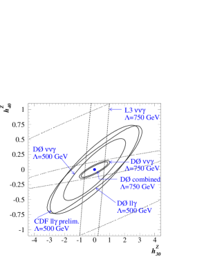
Figure 16: Summary of the 95% CL limits on anomalous CP-conserving $ZZ\gamma$ coupling parameters. The CDF and DØ limits are indicated by the solid contours and the dashed contour indicates the limits from L3 [92] for $\Lambda_{FF}=500$ GeV. The dotted contours show the unitarity limits for $\Lambda_{FF}=500$ GeV (outer contour) and $\Lambda_{FF}=750$ GeV (inner contour).

Limits on the anomalous coupling parameters are obtained using a binned likelihood fit to the photon $E_{T}$ distribution as in the $W\gamma$ analyses. The $Z\gamma$ signal prediction used is based on the leading-order calculation of Baur & Berger [53]. The resulting 95% CL limits on the CP-conserving $ZZ\gamma$ and $Z\gamma\gamma$ coupling parameters are listed in Table 10. Limits on the CP-violating coupling parameters $h_{10}^{V}$ and $h_{20}^{V}$ are numerically the same as the limits on $h_{30}^{V}$ and $h_{40}^{V}$. Figure 16 shows the DØ limits in the $h_{30}^{Z}-h_{40}^{Z}$ and $h_{30}^{\gamma}-h_{40}^{\gamma}$ planes.

5.5.2 THE DØ ANALYSIS OF $p\bar{p}\rightarrow\mbox{${\hbox{$E$\kern-4.80005pt\lower-0.34445pt\hbox{/}}}_{T}$}\gamma+X$

DØ has carried out the first measurement of $Z\gamma$ production in the $Z\rightarrow\nu\bar{\nu}$ decay channel at a hadron collider, and has demonstrated the higher sensitivity of this channel to $ZZ\gamma$ and $Z\gamma\gamma$ anomalous couplings compared with the channel $p\bar{p}\rightarrow\ell^{+}\ell^{-}\gamma+X$ [73, 93]. The neutrino decay channel has several experimental advantages over the $\ell^{+}\ell^{-}\gamma$ channel: the radiative decay background resulting from the emission of a photon from the charged leptons in $Z\rightarrow\ell^{+}\ell^{-}$ decays is not present; the branching fraction is higher, $B(Z\rightarrow\nu\bar{\nu})/B(Z\rightarrow\ell^{+}\ell^{-})\approx 3$, where $\ell=e,\mu$; and the efficiency is high since only one photon has to be detected as opposed to a photon plus two charged leptons.

Although these factors result in a higher sensitivity to anomalous couplings, there are also some disadvantages—there are additional backgrounds, and the $Z$ boson cannot be identified since its mass cannot be reconstructed.

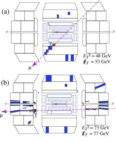
Figure 17: Side views of the DØ calorimeter and tracking systems for events attributed to (a) cosmic ray muon bremsstrahlung and (b) beam halo muon bremsstrahlung. The dashed line indicates the probable muon track, the photon is labeled $\gamma$, and the reconstructed event vertex is indicated by the cross. All cells in the calorimeter with energy greater than 200 MeV are shown.

There are two sources of instrumental backgrounds. One is due to cosmic ray muons or beam halo muons that traverse the detector and emit a photon by bremsstrahlung, which may deposit an energy cluster in the EM calorimeter, as illustrated in Figure 17. If the muon is not reconstructed in the detector, the resulting event signature is a single photon with balancing missing $E_{T}$. The second source is due to $W\rightarrow e\nu$ events in which the electron is misidentified as a photon, which occurs if the electron track is not reconstructed in the central tracking chambers. There are also physics backgrounds from QCD processes: multijet production where a jet is misidentified as a photon and the missing $E_{T}$ is due to mismeasured jets; direct photon production in which a jet contributes to ${\hbox{$E$\kern-6.00006pt\lower-0.43057pt\hbox{/}}}_{T}$; and $Z~{}+$ jets $\rightarrow\nu\bar{\nu}~{}+$ jets events in which a jet is misidentified as a photon.

To reduce the backgrounds from QCD processes and from $W\rightarrow e\nu$, tight requirements are made on the photon $E_{T}$ and the missing transverse energy: $E_{T}^{\gamma}>40$ GeV and $\mbox{${\hbox{$E$\kern-6.00006pt\lower-0.43057pt\hbox{/}}}_{T}$}>40$ GeV. These requirements reduce the QCD backgrounds to negligible levels. However, in $W\rightarrow e\nu$ decays the electron $E_{T}$ distribution has a peak at $E_{T}\approx 40$ GeV, and events in the tail of the Jacobian result in a significant source of background.

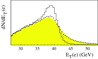
Figure 18: The $E_{T}^{e}$ spectrum for $W\rightarrow e\nu$ events with $p_{T}^{W}=0$ (solid line), with the correct $p_{T}^{W}$ distribution ($\bullet$) and with the DØ detector resolutions (shaded) [from [94]]

Two methods are used to further reduce this background. The first utilizes the fact that the Jacobian edge of the $E_{T}^{e}$ distribution is smeared if the $W$s are produced with significant transverse momentum due to initial-state radiation of gluons, illustrated in Figure 18. The number of electrons with $E_{T}^{e}>40$ GeV is then higher relative to events with lower $p_{T}^{W}$. To suppress the smearing of the Jacobian edge, thereby reducing the $W\rightarrow e\nu$ background, a jet veto is applied, which rejects any event containing a jet with $E_{T}^{j}>15$ GeV. This method has the high efficiency of 85% for retaining $Z(\nu\bar{\nu})\gamma$ events.

The second method, to reject electrons which do not have reconstructed tracks, applies a cut on the number of hits detected in each tracking chamber within a road defined between the electromagnetic cluster’s energy-weighted center and the event vertex. The efficiency of this cut is approximately 75%. This technique gives a rejection factor of $r_{h}\approx 45$ and provides powerful background rejection when combined with the rejection factor for the track match requirement, which has $r_{h}\approx 5$.

The muon bremsstrahlung background is significantly suppressed by applying the following requirements:

1. The electromagnetic energy cluster must point back to the interaction vertex. A straight line $\chi^{2}$ fit is performed using the energy-weighted centers of the EM cluster in all four layers of the calorimeter plus the event vertex position. The resulting probabilities $P_{xy}(\chi^{2})$ and $P_{rz}(\chi^{2})$ in the $xy$ and $rz$ planes are required to be greater than 1%. The vertex resolutions measured using $Z\rightarrow ee$ events are $\sigma_{xy}=11$ cm and $\sigma_{rz}=17$ cm and the efficiency of the $P(\chi^{2})$ requirement is 94%.

2. No reconstructed muon is present in the CF muon chambers ($|\eta|<1.0$). Typically, cosmic ray muons producing bremsstrahlung photons consistent with the interaction vertex traverse the detector in the central region. The efficiency of this requirement is approximately 99%;

3. No muon is identified by an energy deposition in the finely segmented calorimeter, forming a track in a road defined by the energy-weighted center of the EM cluster and the interaction vertex. These events are predominantly from cosmic ray and beam halo muon bremsstrahlung. This requirement has an efficiency of 97%.

Applying all the requirements described above, the total estimated background is $5.8\pm 1.0$ events, with $4.0\pm 0.8$ events from $W\rightarrow e\nu$ and $1.8\pm 0.6$ events from muon bremsstrahlung. The expected number of signal events for the SM and for anomalous couplings is estimated using a leading-order $Z\gamma$ event generator [53] combined with the parametrized DØ detector simulation described previously. For the SM the expected number of signal events is $1.8\pm 0.2$. Four candidate events are observed in the data, consistent with the SM expectations.

Limits on the anomalous couplings are derived from a maximum likelihood fit to the photon $E_{T}$ spectrum, and are listed in Table 10. These limits are the most stringent limits obtained from any one decay channel.

6 PROSPECTS FOR FUTURE STUDIES OF
ANOMALOUS COUPLINGS

The analysis performed at the Tevatron will be repeated at future machines, with increased energy and luminosity, where the data will be much more sensitive to the virtual effects that generate deviations from the SM expressions for the triple gauge boson couplings.

This section reviews the expected sensitivity of experiments at LEPII, the Tevatron, the Large Hadron Collider (LHC) [97], and the Next Linear Collider (NLC) [98]. Various options for collision energies and integrated luminosities have been considered for a linear collider. We provide results for representative cases at the 95% CL (unless stated otherwise).

The expected sensitivity of the NLC will be sufficient to probe the SM radiative corrections (both electroweak and strong) to the processes involving triple boson couplings; the theoretical expectation for all contributions to the effective parameters generated by non-SM physics will be subdominant and must be extracted as deviations from these radiative corrections. We would also like to remark that, for any given process, there are in principle a large number of terms in the effective Lagrangian that generate deviations from the SM predictions. For example, the process $W^{+}W^{-}\rightarrow W^{+}W^{-}$ in the case where light scalars are present is affected by the trilinear vertices involving gauge bosons, as well as by the scalar-$W$ couplings. Moreover, since the initial-state $W$ bosons are radiated from a fermion, the process is also affected by non-SM fermion-$W$ couplings.

6.1 LEP II and the Tevatron

The LEP II experiments each collected $\sim 50$ pb^-1 in 1997 at a CM energy of $183$ GeV. The limits on anomalous couplings from these data are expected to be a factor of about three better than the present LEP II limits (see Table 8). If a total integrated luminosity of 500 pb^-1 per experiment is achieved in the future, the limits on the anomalous couplings will have a precision of $0.02-0.1$ [96].

The expected integrated luminosity at the Tevatron in Run II, which will start in the year 2000, is $\approx 2-4$ fb^-1. Further upgrades in the accelerator complex may result in data samples of up to 30 fb^-1. If 10 fb^-1 is achieved, limits on anomalous couplings are expected to improve by a factor of about five [95]. With $\approx 2-4$ fb^-1 in Run II, the Tevatron also provides a unique opportunity to observe the SM radiation zero in $p\bar{p}\rightarrow W\gamma$.

6.2 LHC

Extracting deviations from the SM from LHC data is complicated by the large contributions generated by the QCD corrections [99, 100]. The expected limits from the reactions $pp\rightarrow WZ,\,W\gamma$ for an integrated luminosity of 100 fb^-1 are [101, 102]

$$|\Delta\kappa_{Z}|<0.07 |\lambda_{Z}|<0.005$$ (24)

$$|\Delta\kappa_{\gamma}|<0.04 |\lambda_{\gamma}|<0.0025$$ (25)

[which differ from the results of Baur et al [103] due to the choice of form factor scale $\Lambda_{FF}$. Fouchez [102] chose $\Lambda_{FF}=10$ TeV which is much larger than the effective $\hat{s}$ of $\sim 1.4$ TeV; Baur et al took $\Lambda_{FF}=1$ or 3 TeV.]

These values will not be sufficient to probe new physics at a scale above the effective CM energy of the hard scattering process. Using the estimates obtained in Section 1.1.2, the above bounds imply that the scale of new physics is larger than $\sim 300$ GeV, while the effective CM energy is $\sim 1.2$ TeV [103]. In other words, there are no models with a scale above $1.2$ TeV that produce deviations larger than those indicated in Equation 25.

Concerning the sensitivity to the neutral vector boson vertices, the LHC is expected to achieve the limits [104]

$$\left|h_{3}^{Z}\right|<2\times 10^{-6}\qquad\left|h_{4}^{Z}\right|<10^{-5}.$$ (26)

6.3 ep Collisions at the LHC

This proposed collider, which would collide protons in the LHC ring with electrons in a reconstructed LEP ring would be able to probe the trilinear gauge boson vertices, but the bounds will not improve on any obtained from LEP II. The bound estimates for an integrated luminosity of 1 fb^-1 at 90% CL are given in Table 11 [105], where collisions of 55 GeV electrons on 8 TeV protons were assumed.

This collider will not be able to probe physics that cannot be directly produced for the integrated luminosity for which these studies were carried out.

6.4 NLC

The planned linear collider will be the first machine that can probe effective parameters at a level allowing derivation of constraints on the scale of new physics superior to those obtained from direct production.

Studies have been done for $e^{+}e^{-}$, $e\gamma$, and $\gamma\gamma$ initial states [the last two using back-scattered lasers [106]]. Although the CM energy of the machine has not been definitely chosen, it is expected to operate at $0.5$ TeV for a first stage and then be upgraded to $1.5$ TeV. There have been various studies of the sensitivity of these machines to the effective couplings in Equation 5 [31, 107, 108, 109]. The most recent of these [108] makes a global 5 parameter fit to the coefficients $\Delta\kappa_{\gamma}$, $Delta\kappa_{Z}$, $\lambda_{\gamma}$, $\lambda_{Z}$, and $\Delta g_{1}^{Z}$ in Equation 5, which we reproduce in Table 12. The table also includes limits for the couplings in Equation 7 [110] obtained using various asymmetries.

The above sensitivity limits are strong enough to insure that the NLC will be able to probe new physics at scales beyond its CM energy. Although this collider will also probe other reactions where new physics effects can be significantly larger, the type of physics that modifies the triple gauge boson vertices might not affect those other observables.

Alhough the above estimates give very tight limits, a complete multiparameter study including initial-state radiation effects and detector efficiencies is still lacking.

7 SUMMARY

We have reviewed studies of the trilinear gauge boson couplings from the Tevatron Run I data, with an integrated luminosity of $\approx 100$ pb^-1. Using gauge boson pair production processes, these measurements provide the first direct tests of the trilinear gauge boson couplings.

Limits on the $WW\gamma$ effective couplings rule out the U(1)_EM-only coupling of the $W$ boson to the photon ($\kappa=\lambda=0$) and also rule out a zero $W$ boson magnetic moment ($\mu_{W}=0$). Studies of $WW$ and $WZ$ production are also sensitive to the $WWZ$ coupling and, for the first time, the Tevatron measurements provide direct evidence for the existence of the $WWZ$ coupling.

A simultaneous fit to the processes sensitive to the $WW\gamma$ and $WWZ$ couplings provides the most stringent direct limits to date on the effective couplings (for $\Lambda_{FF}=2$ TeV and assuming $\Delta\kappa_{\gamma}=\Delta\kappa_{Z},\lambda_{\gamma}=\lambda_{Z}$):

$-0.30<\Delta\kappa<0.43$

$-0.20<\lambda<0.20$

$-0.52<\Delta g^{Z}_{1}<0.78$;

or, in the $\alpha_{B\phi}$, $\alpha_{W\phi}$, $\alpha_{W}$ parametrization:

$-0.73<\alpha_{B\phi}<0.58$

$-0.22<\alpha_{W\phi}<0.44$

$-0.20<\alpha_{W}<0.20$.

Tests of the $ZZ\gamma$ and $Z\gamma\gamma$ effective couplings also provide the most stringent limits to date. For a form factor scale $\Lambda_{FF}=750$ GeV the limits are

$\left|h^{V}_{10,30}\right|<0.36$

$\left|h^{V}_{20,40}\right|<0.05$.

While these measurements do not yet rule out any specific model beyond the SM, the measurements are of crucial importance because they test the trilinear gauge boson couplings, which are a fundamental prediction of the SM, resulting from the non-Abelian nature of the theory. It is worth pointing out that precision measurements of this character have provided some of the most striking breakthroughs in particle physics—examples are the anomalous magnetic moment of the electron and the Dirac theory, and $K^{0}$–$\overline{K}^{0}$ mixing and CP violation.

The typical values for effective couplings in models beyond the SM are at the level $\leq 0.02$ (see Table 2). Therefore, as the precision improves in the future, experiments will yield valuable information about new physics that could give rise to anomalous couplings. The next measurements will be made at LEP II, the Tevatron, the LHC, and the planned NLC. Even if new physics is directly discovered, measurement of the loop corrections to the triliner gauge boson couplings will still provide a critical test of self-consistency of the theory.

ACKNOWLEDGMENTS

We are indebted to the DØ and CDF Collaborations for making their results available to us. J Ellison would like to thank his DØ colleagues who worked on the diboson analyses, as well as Ulrich Baur for many useful, stimulating discussions. We thank Greg Landsberg for providing the event displays used in Figure 17, and Ann Heinson, who carefully read our manuscript and made valuable suggestions. This work was supported by the US Department of Energy.

	oblique	$(g-2)_{\mu}$	$d_{n}$	$d_{e}$	$b\rightarrow s\gamma$	Atomic	$K^{0}_{L}\rightarrow\mu\mu$
	params.	[29, 30]	[31]	[32]	[33]	parity	[34]
	[28]					viol.[34]
$|\Delta\kappa_{\gamma}|$	$0.05$	$1$	–	–	$2$	$1$	$1$
$|\Delta\kappa_{Z}|$	$0.4$	–	–	–	–	$0.12$	–
$|\lambda_{\gamma}|$	$0.2$	$2$	–	–	$7$	$0.13$	–
$|\lambda_{Z}|$	$0.2$	–	–	–	–	$0.13$	–
$|\tilde{\kappa}_{\gamma}|$	–	–	–	$0.14$	$0.4$	–	–
$|\tilde{\kappa}_{Z}|$	–	–	–	$0.04$	–	–	–
$|\tilde{\lambda}_{\gamma}|$	–	–	0.00025	–	$1.3$	–	–
$|g_{4}^{Z}|$	–	–	–	$0.80$	–	–	–
$|h_{3}^{\gamma}|$	–	$4.5$	–	–	–	–	–

Table 1: Indirect upper bounds on the effective parameters from precision measurements.

Model	$|\Delta\kappa_{\gamma}|$	$|\lambda_{\gamma}|$	$|\tilde{\kappa}_{\gamma}|$
standard model	$0.008$ [36, 37]	$0.002$ [37]	$10^{-22}$ [38, 39]
2HDM	$0.016$ [40]	$0.0014$ [40]	–
Multi-doublet	–	–	$4\times 10^{-6}$ [41, 38]
E6	$2.5\times 10^{-5}$ [42]	$0.003$ [42]	–
SUSY	$0.005$ [43]	$5\times 10^{-5}$ [43]	$3\times 10^{-4}$ [44]
TC	$0.002$ [45]	–	$7\times 10^{-6}$ [45]
4th generation	–	–	$5\times 10^{-3}$ [46]

Table 2: Calculated values of the effective parameters in several theoretical models. The abbreviations are 2HDM (two Higgs-doublet model), SUSY (Suppersymmetry), and TC (Technicolor).

	DØ		CDF
	$W\gamma\rightarrow e\nu\gamma$	$W\gamma\rightarrow\mu\nu\gamma$	$W\gamma\rightarrow e\nu\gamma$	$W\gamma\rightarrow\mu\nu\gamma$
Lepton $\eta$	$|\eta_{e}|<1.1$ or	$|\eta_{\mu}|<1.0$	$|\eta_{e}|<1.1$	$|\eta_{\mu}|<0.6$
	$1.5<|\eta_{e}|<2.5$
Lepton $p_{T}$ (GeV$/c$)	$E_{T}^{e}>25$	$p_{T}^{\mu}>15$	$E_{T}^{e}>20$	$p_{T}^{\mu}>20$
Missing $E_{T}$ (GeV)	$\mbox{${\hbox{$E$\kern-4.80005pt\lower-0.34445pt\hbox{/}}}_{T}$}>25$	$\mbox{${\hbox{$E$\kern-4.80005pt\lower-0.34445pt\hbox{/}}}_{T}$}>15$	$\mbox{${\hbox{$E$\kern-4.80005pt\lower-0.34445pt\hbox{/}}}_{T}$}>20$	$\mbox{${\hbox{$E$\kern-4.80005pt\lower-0.34445pt\hbox{/}}}_{T}$}>20$
Photon $\eta$	$|\eta_{\gamma}|<1.1$ or $1.5<|\eta_{\gamma}|<2.5$		$|\eta_{\gamma}|<1.1$
Photon $E_{T}$ (GeV)	$E_{T}^{\gamma}>10$		$E_{T}^{\gamma}>7$
$\ell-\gamma$ separation	$\Delta R_{\ell\gamma}>0.7$		$\Delta R_{\ell\gamma}>0.7$

Table 3: Summary of $W\gamma$ event selection requirements

	DØ		CDF
	92.8 pb-1		67.0 pb-1
	$W\gamma\rightarrow e\nu\gamma$	$W\gamma\rightarrow\mu\nu\gamma$	$W\gamma\rightarrow e\nu\gamma$	$W\gamma\rightarrow\mu\nu\gamma$
$N_{\rm data}$	57	70	75	34
$N_{\rm bkg}$	15.2 $\pm$ 2.5	27.7 $\pm$ 4.7	16.1 $\pm$ 2.4	10.3 $\pm$ 1.2
$N_{\rm sig}$	$41.8^{+8.8}_{-7.5}$	$42.3^{+9.7}_{-8.3}$	$58.9\pm 9.0\pm 2.6$	$23.7\pm 5.9\pm 1.1$
$N_{\rm SM}$	43.6 $\pm$ 3.1	38.2 $\pm$ 2.8	$53.5\pm 6.8$	$21.8\pm 4.3$

Table 4: Number of candidate $W\gamma$ events observed $N_{\rm data}$. $N_{\rm bkg}$, estimated background; $N_{\rm sig}$, number of signal events after background subtraction; $N_{\rm SM}$, SM prediction

	DØ			CDF
	$e\nu e\nu$	$e\nu\mu\nu$	$\mu\nu\mu\nu$	(all modes)
Electron $\eta$	$|\eta_{e}|<1.1$ or			$|\eta_{e}|<1.0$ or
	$1.5<|\eta_{e}|<2.5$			$1.20<|\eta_{e}|<1.35$
Muon $\eta$	$|\eta_{\mu}|<1.0$			$|\eta_{\mu}|<1.2$
Lepton $p_{T}$ (GeV$/c$)	$E_{T}^{e1}>25$	$E_{T}^{e}>25$	$p_{T}^{\mu 1}>25$	$p_{T}>20$
	$E_{T}^{e2}>20$	$p_{T}^{\mu}>15$	$p_{T}^{\mu 2}>20$	(for all $e$’s, $\mu$’s)
Missing $E_{t}$ (GeV)	$\mbox{${\hbox{$E$\kern-4.80005pt\lower-0.34445pt\hbox{/}}}_{T}$}>25$	$\mbox{${\hbox{$E$\kern-4.80005pt\lower-0.34445pt\hbox{/}}}_{T}$}>20$	$-$	$\mbox{${\hbox{$E$\kern-4.80005pt\lower-0.34445pt\hbox{/}}}_{T}$}>20$
$t\bar{t}$ rejection	$E_{T}^{\rm had}<40$ GeV			no jets with
				$E_{T}>10$ GeV
$Z$ rejection	see text			see text

Table 5: Summary of $WW\rightarrow\ell\nu\ell^{\prime}\nu^{\prime}$ event selection requirements.

	DØ	CDF
Electron $\eta$	$|\eta_{e}|<1.1$ or	$|\eta_{e}|<1.1$ or
	$1.5<|\eta_{e}|<2.5$	$1.1<|\eta_{e}|<2.4$
Muon $\eta$	–	$|\eta_{\mu}|<1.0$
Lepton $E_{T}$ or $p_{T}$ (GeV)	$E_{T}^{e}>25$	$E_{T}^{e}$, $p_{T}^{\mu}>20$
Missing $E_{t}$ (GeV)	$\mbox{${\hbox{$E$\kern-4.80005pt\lower-0.34445pt\hbox{/}}}_{T}$}>25$	$\mbox{${\hbox{$E$\kern-4.80005pt\lower-0.34445pt\hbox{/}}}_{T}$}>20$
Transverse mass (GeV$/c^{2}$)	$m_{T}(\ell;\mbox{${\hbox{$E$\kern-4.80005pt\lower-0.34445pt\hbox{/}}}_{T}$})>40$	$m_{T}(\ell;\mbox{${\hbox{$E$\kern-4.80005pt\lower-0.34445pt\hbox{/}}}_{T}$})>40$
Jet cone radius	$R=0.3$ (Ia), 0.5 (Ib)	$R=0.4$
Jet $\eta$	$|\eta_{j}|<2.5$	$|\eta_{j}|<2.5$
Jet $E_{T}$	$E_{T}^{j}>20$	$E_{T}^{j}>30$
Dijet invariant mass (GeV$/c^{2}$)	$50<m_{jj}<110$	$60<m_{jj}<110$
Dijet $p_{T}$ (GeV$/c$)	–	$p_{T}^{jj}>200$

Table 6: Summary of $WW/WZ\rightarrow\ell\nu jj$ event selection requirements

Coupling	$\Lambda_{FF}=1.5$ TeV	$\Lambda_{FF}=2.0$ TeV
$\Delta\kappa_{\gamma}=\Delta\kappa_{Z}$	$-$0.33, 0.46	$-$0.30, 0.43
$\lambda_{\gamma}=\lambda_{Z}$	$-$0.21, 0.21	$-$0.20, 0.20
$\Delta\kappa_{\gamma}$ (HISZ)	$-$0.39, 0.61	$-$0.37, 0.56
$\lambda_{\gamma}$ (HISZ)	$-$0.21, 0.21	$-$0.20, 0.20
$\Delta g^{Z}_{1}$ (SM $WW\gamma$)	$-$0.56, 0.86	$-$0.52, 0.78
$\Delta\kappa_{Z}$ (SM $WW\gamma$)	$-$0.46, 0.64	$-$0.42, 0.59
$\lambda_{Z}$ (SM $WW\gamma$)	$-$0.33, 0.37	$-$0.31, 0.34
$\Delta\kappa_{\gamma}$ (SM $WWZ$)	$-$0.63, 0.75	$-$0.59, 0.72
$\lambda_{\gamma}$ (SM $WWZ$)	$-$0.27, 0.25	$-$0.26, 0.24

Table 7: DØ limits on anomalous couplings at the 95% CL from a simultaneous fit to the $W\gamma$, $WW\rightarrow\ell\nu\ell^{\prime}\nu^{\prime}$, and $WW/WZ\rightarrow e\nu jj$ data.

Coupling	$\Lambda_{FF}=1.5$ TeV	$\Lambda_{FF}=2.0$ TeV	LEP combined
$\alpha_{B\phi}$	$-$0.76, 0.61	$-$0.73, 0.58	$-$0.81, 1.50
$\alpha_{W\phi}$	$-$0.24, 0.46	$-$0.22, 0.44	$-$0.28, 0.33
$\alpha_{W}$	$-$0.21, 0.21	$-$0.20, 0.20	$-$0.37, 0.68
$\Delta g^{Z}_{1}$	$-$0.31, 0.60	$-$0.29, 0.57	$-$

Table 8: DØ limits on anomalous couplings $\alpha_{B\phi}$, $\alpha_{W\phi}$, $\alpha_{W}$, and $\Delta g^{Z}_{1}$ at the 95% CL from a simultaneous fit to the $W\gamma$, $WW\rightarrow\ell\nu\ell^{\prime}\nu^{\prime}$, and $WW/WZ\rightarrow e\nu jj$ data. The last column gives the combined limits from the LEP experiments [88]. The LEP limits should be multiplied by a factor $(1+s/\Lambda^{2}_{FF})^{2}$ to compare directly with the DØ results. At the LEP energy $\sqrt{s}=172$ GeV, this factor is only 1.026 for $\Lambda_{FF}=1.5$ TeV so the numbers in the table have not been corrected.

	DØ		CDF
	$Z\gamma\rightarrow ee\gamma$	$Z\gamma\rightarrow\mu\mu\gamma$	$Z\gamma\rightarrow ee\gamma$	$Z\gamma\rightarrow\mu\mu\gamma$
$\int{\cal L}dt$ (pb${}^{-1})$	111.3	100.7	67.0	67.0
$N_{\rm data}$	18	17	18	13
$N_{\rm bkg}$	$2.24\pm 0.54$	$3.62\pm 0.68$	$0.9\pm 0.3$	$0.5\pm 0.1$
$N_{\rm sig}$	$15.8^{+4.9}_{-4.3}$	$13.4^{+4.7}_{-4.1}$	$17.1\pm 5.7$	$12.5\pm 3.6$
$N_{\rm SM}$	$16.0\pm 1.3$	$18.6\pm 2.0$	$16.2\pm 1.8$	$8.7\pm 0.7$

Table 9: $N_{\rm data}$, the number of candidate $Z\gamma$ events observed; $N_{\rm bkg}$, the estimated background; $N_{\rm sig}$, the number of signal events after background subtraction; $N_{\rm SM}$, the SM prediction.

Analysis	$\int{\cal L}dt$ (pb-1)	$\Lambda_{FF}$ (GeV)	$h^{Z}_{30}$	$h^{Z}_{40}$
CDF Ia $\ell^{+}\ell^{-}\gamma$	20	500	$-$3.0, 2.9	$-$0.7, 0.7
CDF Ia + Ib prelim.	67	500	$-$1.6, 1.6	$-$0.4, 0.4
DØ Ia $\ell^{+}\ell^{-}\gamma$	14	500	$-$1.8, 1.8	$-$0.5, 0.5
DØ Ia $\nu\bar{\nu}\gamma$	13	500	$-$0.87, 0.87	$-$0.19, 0.19
”	”	750	$-$0.49, 0.49	$-$0.07, 0.07
DØ Ib $\ell^{+}\ell^{-}\gamma$	97 ($e$), 87($\mu$)	500	$-$1.31, 1.31	$-$0.26, 0.26
”	”	750	$-$0.67, 0.67	$-$0.08, 0.08
DØ combined	–	750	$-$0.36, 0.36	$-$0.05, 0.05

Table 10: Summary of the 95% CL limits on anomalous couplings from the $Z\gamma$ analyses. All couplings other than those indicated are held to their SM values. Limits on the CP-violating coupling parameters $h_{10}^{V}$ and $h_{20}^{V}$ are numerically the same as the limits on $h_{30}^{V}$ and $h_{40}^{V}$. Limits on the couplings $h_{10}^{\gamma}-h_{40}^{\gamma}$ are almost the same as those on $h_{10}^{Z}-h_{40}^{Z}$.

LEP$\times$LHC expected limits
$|\lambda_{\gamma}|<0.12$	$|\lambda_{Z}|<0.3$	$|\tilde{\lambda}_{\gamma}|<0.12$
$|\tilde{\lambda}_{Z}|<0.24$	$|\Delta\kappa_{\gamma}|<0.4$	$|\Delta\kappa_{Z}|<0.8$	$|\tilde{\kappa}_{Z}|<1$
$|g_{4}^{Z}|<0.35$	$|g_{5}^{Z}|<0.5$	$-0.6<g_{1}^{Z}<0.3$

Table 11: Expected limits on effective couplings at the 90% CL for the LHC$\times$LEP collider with an integrated luminosity of 1 fb^-1. The reactions studied are $e^{-}p\rightarrow e^{\pm}W^{\mp}X$, and $\nu ZX$

$\sqrt{s}$:	0.5 TeV	1 TeV			0.5 TeV	1 TeV
$|\Delta\kappa_{\gamma}|$	0.002	0.0006		$|g_{4}^{Z}|$	0.075	0.0024
$|\Delta\kappa_{Z}|$	0.05	0.02		$|h_{1}^{\gamma}|$	0.003	–
$|\lambda_{\gamma}|$	0.011	0.003		$|h_{1}^{Z}|$	0.02	–
$|\lambda_{Z}|$	0.025	0.006		$|h_{3}^{V}|$	0.03	0.005
$|\Delta g_{1}^{Z}|$	0.05	0.015		$|h_{4}^{V}|$	0.003	0.0002

Table 12: Expected limits on the effective couplings from the initial and intermediate stages of the NLC. Luminosities for the $WW\gamma$ and $WWZ$ coupling parameters are 20 and 50 fb^-1 for 0.5 and 1 TeV CM energies respectively. Limits on the C odd, P even parameter $g_{4}^{Z}$ [99] are derived from the asymmetries in $e^{+}e^{-}\rightarrow\nu\bar{\nu}Z$ [109], for luminosities of 10 fb^-1 and 100 fb^-1. They hold for energies in the range 0.3–2 TeV.

Figure 2: Leading-order Feynman diagram for $W$ production with radiative $W$ decay: The charged lepton radiates a photon by bremsstrahlung.

Figure 3: Photon transverse momentum spectra for (a) $W\gamma$ production and (b) $Z\gamma$ production at the Tevatron for SM and anomalous couplings. From Refs. [51] and [52].

Figure 9: Limits on the $WW\gamma$ couplings at the 95% confidence level (CL) for $\Lambda_{FF}=1.5$ TeV from DØ (ellipse). The shaded bands are the regions allowed by the 95% CL limits from the CLEO and ALEPH observations of $b\rightarrow s\gamma$ decays [78].

Figure 10: Limits on the $W$ boson magnetic dipole moment $\mu_{W}$ and electric quadrupole moment $Q_{W}$ at the 95% confidence level from DØ (ellipse). The shaded bands are the limits from $b\rightarrow s\gamma$ [78].

Figure 15: Kinematic properties of the candidate events and estimated backgrounds in the DØ $Z(\ell^{+}\ell^{-})\gamma$ analysis: (a) photon tranverse energy for the combined $ee\gamma$ and $\mu\mu\gamma$ samples; (b) dielectron invariant mass; (c) dielectron-photon invariant mass.

References

- [1]
- [2]
- [3] Weinberg S. Phys. Rev. Lett. 19:1264 (1967). Salam A. In Elementary Particle Theory, ed. N Svarthom, et al. Stockholm: (1968); Peskin ME, Schroeder DV. An Introduction to Quantum Field Theory. Addison-Wesley (1995); Weinberg S. The Quantum Theory of Fields. Cambridge, UK: Cambridge Univ. Press (1995)
- [4] Baur U, Errede S, Muller T, eds. Proc. Int. Symp. Vector Boson Self-interact. Am. Inst. Phys. (1996) (AIP Conf. Proc. 350)
- [5] Weinberg S. Physica A 96:327 (1979); Georgi H. Nucl. Phys. B361:339 (1991), Nucl. Phys. B363:301 (1991); Pich A. In Mex. Sch. Part. Fields, 5th, Guanajuato, Mex., Nov. 30–Dec 11, 1992, ed. JL Lucio, M Vargas. Am. Inst. Phys. (1994) (AIP Conf. Proc., v. 317)
- [6] Weinberg S. In Conference on Historical and Philosophical Reflections on the Foundation of Quantum Field Theory, Boston, MA, Mar. 1–3, 1996 (e-print archive: hep-th/9702027)
- [7] Proc. Int. Europhys. Conf. High Energy Phys., Aug. 19–26, 1997, Jerusalem, Israel; Proc. 1996 DPF/DPB Summer Stud. New Dir. High-Energy Phys. (Snowmass 96), Snowmass, CO, Jun. 25–Jul. 12, 1996, ed. DG Cassel, L Trindle Gennari, RH Siemann (Stanford Linear Accelerator Center, 1997); Proc. Int. Conf. Phys. Beyond Standard Model, 5th, Balholm, Norway, Apr. 29–May 4, 1997
- [8] Barnett RM, et al. Phys. Rev. D 54:1 (1996)
- [9] Weinberg S. Physica A 96:327 (1979); Chanowitz MS, Gaillard MK. Nucl. Phys. B261:379 (1985); Chanowitz M, Golden M, Georgi H. Phys. Rev. Lett. 57:2344 (1986)
- [10] Frere JM, et al. Phys. Lett. B 292:348 (1992); Nucl. Phys. B429:3 (1994)
- [11] Perez MA, Toscano JJ, Wudka J. Phys. Rev. D 52:494 (1995)
- [12] Veltman M. Acta Phys. Pol. B12:437 (1981)
- [13] Arzt C, Einhorn MB, Wudka J, Phys. Rev. D 49:1370 (1994)
- [14] Georgi H. Nucl. Phys. B361:339 (1991), Nucl. Phys. B363:301 (1991); De Rujula A, et al. Nucl. Phys. B384:3 (1992); Arzt C. Phys. Lett. B 342:189 (1995)
- [15] Buchmuller W, Wyler D, Nucl. Phys. B268:621 (1986)
- [16] Hagiwara K, et al. Nucl. Phys. B282:253 (1987)
- [17] Renard FM, Nucl. Phys. B196:93 (1982)
- [18] Gounaris G, et al. “Triple Gauge Boson Couplings” in Proceedings of the CERN Workshop on LEP II Physics, ed. Altarelli G et al, CERN 96-01, Vol. 1, p.525 (1996)
- [19] Longhitano AC. Phys. Rev. D 22:1166 (1980); Nucl. Phys. B188:118 (1981); Holdom B. Phys. Lett. B 258:156 (1991); Appelquist T, Wu G-H. Phys. Rev. D 48:3235 (1993); Phys. Rev. D 51:240 (1995)
- [20] Hagiwara K, et al. Phys. Rev. D 48:2182 (1993)
- [21] Arzt C, Einhorn MB, Wudka J. Nucl. Phys. B433:41 (1995)
- [22] Wudka J. Int. J. Mod. Phys. A9:2301 (1994)
- [23] Weinberg S. Physica A 96:327 (1979); Georgi H, Manohar A. Nucl. Phys. B234:189 (1984); Georgi H. Phys. Lett. B 298:187 (1993)
- [24] Polchinski J. Recent Directions in Particle Theory: From Superstrings and Black Holes to the Standard Model (TASI 92) Boulder, CO, Jun 3–28, 1992, ed. J Harvey, J Polchinski. World Scientific (1993)
- [25] Baur U, Berger EL. Phys. Rev. D 47:4889 (1993); Golden M, Han T, Valencia G. In Electroweak Symmetry Breaking and New Physics at the TeV Scale, ed. TL Barklow, et al. World Scientific, Singapore (1996)
- [26] For similar calcualtions see A. Culatti, et al., in Physics with Linear Colliders (The European Working Groups 4 Feb - 1 Sep 1995: Session 1), Annecy, France, 4 Feb 1995, and to 3rd Workshop on Physics and Experiments with Linear Colliders (LCWS 95), Iwate, Japan, 8-12 Sep 1995. F. Feruglio and S. Rigolin, Phys. Lett. B 397:245 (1997)
- [27] Grossman Y, Ligeti Z, Nardi E. Nucl. Phys. B465:369 (1996) Nucl. Phys. B480:753 (1996)
- [28] Alam S, Dawson S, Szalapski R. Phys. Rev. D 57:1577 (1998)
- [29] Grau A, Grifols JA. Phys. Lett. B 154:283 (1985); Spagnolo S. Report INFN-TH-97-01 (unpublished) Herzog F. Phys. Lett. B 148:355 (1984), Phys. Lett. B 155:468 (1985)
- [30] Baur U, Berger EL. Phys. Rev. D 47:4889 (1993)
- [31] Boudjema F, et al. Phys. Rev. D 43:2223 (1991)
- [32] Marciano WJ, Queijeiro A. Phys. Rev. D 33:3449 (1986); De Rujula A, et al. Nucl. Phys. B384:3 (1992) He XG, Ma JP, McKellar BHJ. Phys. Lett. B 304:285 (1993)
- [33] Numata K. Z. Phys. C 52:691 (1991); Baur U. In Workshop B Phys. Hadron Accel., Snowmass, CO, Jun. 21–Jul. 2, 1993, ed. CS Mishra, P McBride. Fermilab (1994) (SSCL-SR-1225,C93/06/21); Hewett JL. In Spin Structure in High Energy Processes, ed. L DePorcel, C Dunwoodie. SLAC (1994) (SLAC-Report-444,C93/07/26) Sinha N, Sinha R. Report IMSC-97-03-08 (unpublished) (e-print archive: hep-ph/9707416)
- [34] Godfrey S, Konig H. Phys. Rev. D 45:3196 (1992)
- [35] Cornwall JM. In Fr.-Am. Sem. Theor. Aspects Quantum Chromodynamics, Marseille, France, Jun. 9–13, 1981, ed. JW Dash. (CPT-81/P-1345,C81/06/09.1); Phys. Rev. D 26:1453 (1982); Argyres EN, et al. Nucl. Phys. B391:23 (1993); Papavassiliou J, Philippides K. Phys. Rev. D 48:4255 (1993)
- [36] Papavassiliou J, Philippides K. Phys. Rev. D 48:4255 (1993)
- [37] Kodaira J, et al. In INS Workshop Phys. , and Collis. at Linear Accel., Tokyo, Japan, Dec. 20–22, 1994, ed. Z Hioki, T Ishii, R Najima. Tokyo Univ., Inst. Nucl. Study (1995)
- [38] Chang D, Keung W-Y, Nucl. Phys. B355:295 (1991)
- [39] Khriplovich IB, Pospelov ME. Nucl. Phys. B420:505 (1994)
- [40] Couture G, et al. Phys. Rev. D 36:859 (1987)
- [41] He X-G, McKellar BHJ. Phys. Rev. D 42:3221 (1990), Phys. Rev. D 50:4719 (1994)
- [42] Couture G, Ng JN Z. Phys. C 35:65 (1987)
- [43] Argyres EN, et al. Phys. Lett. B 383:63 (1996)
- [44] Kadoyoshi T, Oshimo N. Phys. Rev. D 55:1481 (1997)
- [45] Appelquist T, Wu G-H. Phys. Rev. D 48:3235 (1993); Phys. Rev. D 51:240 (1995)
- [46] Burgess CP, Pilaftsis A. Phys. Lett. B 333:427 (1994)
- [47] Chang D, Keung W-Y, Pal PB. Phys. Rev. D 51:1326 (1995)
- [48] Barroso A, Boudjema F, Cole J, Dombey N. Z. Phys. C 28:149 (1985)
- [49] Mikaelian KO, Phys. Rev. D17:750 (1978); Brown RW, Sahdev D, Mikaelian KO, Phys. Rev. D20:1164 (1979); Mikaelian KO, Samuel MA, Sahdev D, Phys. Rev. Lett. 43:746 (1979); Zhu Dongpei, Phys. Rev. D22:2266 (1980); Goebel CJ, Halzen F, Leveille JP, Phys. Rev. D23:2682 (1981); Brodsky SJ, Brown RW, Phys. Rev. Lett. 49:966 (1982); Smauel MA, Phys. Rev. D27:2724 (1983); Brown RW, Kowalski KL, Brodsky SJ, Phys. Rev. D28:624 (1983); Bilchak CL, Brown RW, Stroughair JD, Phys. Rev. D29:375 (1984); Cortes J, Hagiwara K, Herzog F, Nucl. Phys. B278:26 (1986); Wallet JC, Z. Phys. C30:575 (1986)
- [50] Baur U, Zeppenfeld D. Nucl. Phys. B308:127 (1988)
- [51] Baur U, Berger EL. Phys. Rev. D41:1476 (1990)
- [52] Baur U, Han T, Ohnemus J. hep-ph/9710416 (1997)
- [53] Baur U, Berger EL. Phys. Rev. D47:4889 (1993)
- [54] Baur U, Errede S, Ohnemus J. Phys. Rev. D48:4103 (1993)
- [55] Hagiwara K, Woodside J, Zeppenfeld D. Phys. Rev. D41:2113 (1990)
- [56] Ohnemus J. Phys. Rev. D47:940 (1993)
- [57] Ohnemus J. Phys. Rev. D44:1403 (1991)
- [58] Ohnemus J. Phys. Rev. D44:3477 (1991)
- [59] Baur U, Han T, Ohnemus J. Phys. Rev. D48:5140 (1993)
- [60] Baur U, Han T, Ohnemus J. Phys. Rev. D53:1098 (1996)
- [61] Baur U, Han T, Ohnemus J. Phys. Rev. D51:3381 (1995)
- [62] Baur U, Zeppenfeld D. Phys. Lett. B201:383 (1988)
- [63] Abe F, et al (CDF Collaboration). Fermilab-Pub-94/244-E (1994)
- [64] Thompson J. Fermilab TM-1909 (1994)
- [65] Edwards H. Ann. Rev. Nucl. Part. Sci. 35:605 (1985)
- [66] Church MD, Marriner JP. Ann. Rev. Nucl. Part. Sci. 43:253 (1993)
- [67] Abe F, et al (CDF Collaboration). Nucl. Instr. and Meth. A271:387 (1988)
- [68] Abachi S, et al (DØ Collaboration). Nucl. Instr. and Meth. A338:185 (1994)
- [69] Nodulman LJ. In Int. Conf. High Energy Phys., 28th, Warsaw, Poland (1996)
- [70] Abe F et al (CDF Collaboration). Phys. Rev. D50:2966 (1994)
- [71] Abe F, et al (CDF Collaboration). Phys. Rev. Lett. 74:1936 (1995)
- [72] Abachi S, et al (DØ Collaboration). Phys. Rev. Lett. 75:1034 (1995)
- [73] Abachi S, et al (DØ Collaboration). Phys. Rev. D56:6742 (1997)
- [74] Abachi S, et al (DØ Collaboration). Phys. Rev. Lett. 78:3634 (1997)
- [75] Benjamin D. In “Topical Workshop Proton-Antiproton Collider Phys., 10th,” Batavia, IL. AIP Conference Proceedings 357, ed. Raja R, Yoh J, p.370. (1996)
- [76] Cousins D, Highland V. Nucl. Instr. Meth. A320:331 (1992)
- [77] Landsberg GL. Ph.D. Thesis, State Univ. NY Stony Brook (1994)
- [78] Drell PS. In “Int. Symp. Lepton-Photon Interact., XVIIIth”, Hamburg, Germany (1997)
- [79] Abachi S, et al (DØ Collaboration). Phys. Rev. Lett. 75:1023 (1995)
- [80] Abe F, et al (CDF Collaboration). Phys. Rev. Lett. 78:4536 (1997)
- [81] Yasuda T. In “Hadron Collider Physics XII”, Stony Brook, NY (1997)
- [82] Abe F, et al (CDF Collaboration). Phys. Rev. Lett. 75:1017 (1995)
- [83] Abachi S et al (DØ Collaboration). Phys. Rev. Lett. 77:3303 (1996)
- [84] Abachi S, et al (DØ Collaboration). Phys. Rev. Lett. 79:1441 (1997)
- [85] Berends FA, et al. Nucl. Phys. B357:32 (1991)
- [86] Marchesini G, et al. Comput. Phys. Commun. 67:465 (1992)
- [87] Brun R, et al. geant User’s Guide v3.14, CERN Program Libr.
- [88] Ward D. In “Int. Europhys. Conf. High Energy Phys.,” Jerusalem, Israel (1997)
- [89] Abe F, et al (CDF Collaboration). Phys. Rev. Lett. 74:1941 (1995)
- [90] Abachi S, et al (DØ Collaboration). Phys. Rev. Lett. 75:1028 (1995)
- [91] Abbott B, et al (DØ Collaboration). Fermilab-Pub-97/363-E (1997). Phys. Rev. D In press
- [92] Acciarri M, et al (L3 Collaboration). Phys. Lett. B412:201 (1997)
- [93] Abachi S, et al (DØ Collaboration). Phys. Rev. Lett. 78:3640 (1997)
- [94] Abbott B, et al (DØ Collaboration). Fermilab-Pub-97/422-E (1997). Phys. Rev. D In press
- [95] Amidei D, Brock R, eds. Fermilab-Pub-96/082 (1996)
- [96] Ajaltouni Z, et al. In Physics at LEP2, ed. G Altarelli, T Sjöstrand. CERN 96-01 (1996)
- [97] Womersley J. In Int. Workshop Fundam. Probl. High-Energy Phys. Field Theory, 20th, Protvino, Russia, June 24–26, 1997 Hinchliffe I. In ITP Conf. Future High Energy Colliders, Santa Barbara, CA, Oct. 21–25, 1996, ed. Z Parsa (Am. Inst. Phys., 1997) (AIP Conf. Proc., 397)
- [98] Kuhlman S, et al (NLC ZDR Design Group and NLC Phys. Working Group). Rep. SLAC-R-0485 (e-print archive: hep-ex/9605011)
- [99] Baur U, Han T, Ohnemus J. Rep. UB-HET-97-03 (unpublished) (e-print archive: hep-ph/9710416)
- [100] Abraham KJ, Lampe B. Rep. MPI-PHT-98-10 (unpublished) (e-print archive: hep-ph/9801400)
- [101] Hinchliffe I, Womersley J. In 1996 DPF/DPB Summer Stud. New Dir. High-Energy Phys. (Snowmass 96), Snowmass, CO, Jun. 25–Jul. 12 1996, ed. DG Cassel, L Trindle Gennari, RH Siemann (Stanford Linear Accelerator Center, 1997)
- [102] Fouchez D. ATLAS internal note PHYS-NO-160 (1994)
- [103] Baur U, Han T, Ohnemus J. Phys. Rev. D 53:1098 (1996)
- [104] Baur U, Han T, Ohnemus J. Rep. UB-HET-97-03 (unpublished) (e-print archive: hep-ph/9710416)
- [105] Baur U, et al. In Large Hadron Collider Workshop (LHC), Aachen, Germany, Oct. 4–9, 1990, ed. G Jarlskog, D Rein, p.570, CERN 90-10 (1990)
- [106] Ginzburg IF, et al. Nucl. Instrum. Methods Al219:5 (1984) Telnov VI. Nucl. Instrum. Methods A294:72 (1990)
- [107] Likhoded AA, Valencia G, Yushchenko OP. Rep. BINP-97-11 (unpublished) (e-print archive: hep-ph/9711325) Boudjema F et al. Phys. Rev. D 43:2223 (1991) de Campos F, et al. Phys. Rev. D 56:4384 (1997) Boudjema F. In Workshop Phys. Exper. Linear Colliders, Morioka-APPI, Japan, Sep. 8–12, 1995, ed. A Miyamoto, et al. World Sci. (1996) Baillargeon M, Belanger G, Boudjema F. Nucl. Phys. B500:224 (1997)
- [108] Pankov AA, Paver N. In Workshop Collis. TeV Energies: Phys. Potential, Annecy, France, Feb. 4, 1995: Session 1 (Session 2: Jul. 2–3, 1995, Assergi, Italy; Session 3: Aug. 30–Sep. 1, 1995, Hamburg, Germany), ed. PM Zerwas. DESY (1996)
- [109] Rindani SD, Singh JP. Report FTUV-97-12 (unpublished) (e-print archive: hep-ph/9703380)
- [110] Choudhury D, Rindani SJ. Phys. Lett. B 335:198 (1994); Rizzo TG. In 1996 DPF/DPB Summer Stud. New Dir. High-Energy Phys. (Snowmass 96), Snowmass, CO, Jun 25–Jul. 12, 1996, ed. DG Cassel, L Trindle Gennari, RH Siemann. SLAC (1997)