1 Introduction

In the case of $\mbox{e}^{+}\mbox{e}^{-}$ annihilation processes the asymptotic collinear and infrared contributions to gluon cross sections can be described in Double Leading Log Approximation (DLLA) by a Markov process (see [1] for a review). This semi-classical description takes into account soft gluon interference effects on the basis of the angular ordering prescription when the parton emission is described by successive branchings and the available phase space is reduced to ever smaller angular regions (color coherence effects). The corresponding QCD master equation is an integral one and is based on Dokshitzer-Gribov-Lipatov-Altarelli-Parisi energy-distribution kernels.

In the framework of this description, progress has been made in obtaining angular scale-invariant correlations between partons [2] (see [3] for a review). This approach, by conception, is a correlation one, based on the method of characteristic functionals. Hence, to derive directly measurable quantities such as normalized factorial moments or factorial cumulants, one needs to perform an integration of the correlation functions over the restricted phase-space region under study. This is possible only after the use of many approximations and by identifying the phase-space regions which give the leading contributions [3].

Apart from this problem, there are also more basic questions which restrict the direct comparison of the QCD correlation approach with experimental data. Firstly, the perturbative QCD calculations deal with an asymptotic behavior of the multiparton correlations valid only for very high energies. In an idealized jet, therefore, finite parton multiplicities in small phase-space bins and energy-momentum conservation effects are systematically ignored [2]. This is one of the most important reasons leading to disagreements between the analytical predictions and $\mbox{e}^{+}\mbox{e}^{-}$ data [4, 5]. Secondly, the increase of the coupling constant for very small phase-space regions sets a limit for the validity of perturbative QCD. Thirdly, non-perturbative effects such as hadronization, resonance decays and Bose-Einstein correlations complicate the comparison of theoretical many-particle inclusive densities with the data even at LEP1 energies [4, 5].

In this paper, therefore, we propose a new way to study the correlations in terms of fluctuations in the multihadronic systems produced in high-energy processes. Being based on a fluctuation approach to intermittency phenomenon (see recent reviews [6, 7] on the subject of intermittency), the model a priori takes into account the finiteness of the number of particles in a single event (finite energies). In order to describe the local multiplicity fluctuations, we adopted the differential Markov equation for parton branching, which has been used to describe global multiplicity fluctuations in high-energy physics in [8, 9, 10, 11] (see also references in [7]).

One of the key ideas of this approach is that, in contrast to a full phase space, a Markov branching process inside a small phase-space window of size $\delta$ can be characterized by a probability $P_{n}(t,\delta)$ of detecting $n$ particles, in which a dependence on an evolution parameter $t$ can be factorized from a phase-space $\delta$-dependence (see Sect. 2). As a consequence of this assumption, the scale-invariant fluctuations experimentally observed inside jets [12] may be considered as a result of fractal phase-space distribution for each particle emitted in successive Markov branchings (Sect. 3). Such an idea ultimately leads to the possibility of taking into account an inhomogeneity of the parton correlations inside a jet and a fairly good quantitative agreement with the $\mbox{e}^{+}\mbox{e}^{-}$-annihilation data [12] and the JETSET 7.4 PS model [13] (Sect. 4).

2 Statistical treatment of branchings

2.1 Global equation

At high energies, gluons dominate the parton-parton cross section due to the large color factor and the infrared singularity. This means that a good high-energy approximation should consider gluon branching only. For generality, however, we shall consider both gluons and quarks treating them as partons.

Let $t$ be the evolution parameter of the parton branching process. The $t$ can be related to the parton virtuality $Q$ and can be defined in the usual way [8, 9, 10, 11]. However, hereafter we shall never refer to the explicit form of this parameter and shall regard it as representing the extent of branching or just time. We assume that the branching process starts with $t=0$ and continues until some $t_{\mbox{max}}$ determined by a QCD cut-off $Q_{0}$. The initial condition for the probability distribution $P_{n}(t)$ of having $n$ particles radiated by the initial one is

$$P_{n=0}(t=0)=1,\qquad P_{n\neq 0}(t=0)=0.$$ (1)

In the following we shall see that, under the assumptions to be made below, the structure of local fluctuations depends neither on the particular definition of the evolution parameter, nor on the initial conditions. The purpose of the introduction of (1) is only to give an illustration of the notion of a typical initiation of the cascade and its further evolution.

A probabilistic scheme [1] of the perturbative parton shower is based on classical picture of the Markov chains of independent parton splittings. Each elementary parton decay depends on just the nearest “forefather”. Let us define $W_{1}\mbox{d}t$ as the probability of branching $a\to b+c$ during a small range of $t$, $\mbox{d}t$, according to one of the following decays: $\mathrm{g}\to\mathrm{g}\mathrm{g}$, $\mathrm{q}\to\mathrm{q}\mathrm{g}$, and $\mathrm{g}\to\bar{\mathrm{q}}\mathrm{q}$. The infinitesimal probability $W_{1}$ in the leading log picture can be written as

$$W_{1}=\sum_{a,b}\int_{0}^{1}{\mbox{d}}z\frac{\alpha_{s}}{2\pi}P_{a\to bc}(z),$$ (2)

where $\alpha_{s}$ is the strong coupling constant and $P_{a\to bc}(z)$ are the Dokshitzer-Gribov-Lipatov-Altarelli-Parisi energy-distribution kernels. The sum runs over all allowed parton branchings. For our simplified model, we will consider the case with $\alpha_{s}=const$, so that $W_{1}$ is a (divergent) constant which does not depend on $t$.

If there are $n$ partons, the probability of the parton emission increases. Let $W_{n}\mbox{d}\,t$ be the probability that the parton system with multiplicity $n$ radiates a new parton during the infinitesimal interval ($t$, $t+\Delta t$). Generally, $W_{n}$ depends on the parton multiplicity $n$. This can be taken into account as

$$W_{n}=w(n)W_{1},\qquad w(1)=1,$$ (3)

where $w(n)$ is a function of $n$ reflecting an increase of the parton radiation. Then the Markov pure birth evolution equation for the multiplicity distribution $P_{n}(t)$ of having $n$ partons at time $t$ is well-known [14]:

$$\frac{\partial P_{n}(t)}{\partial t}=W_{n-1}P_{n-1}(t)-W_{n}P_{n}(t).$$ (4)

The solution of this equation is a global multiplicity distribution $P_{n}(t)$. Since the equation contains ingredients of perturbative QCD, an essential point is to regularize $W_{1}$ and consider the branching evolution up to $t_{\mbox{max}}$ determined by the QCD cut-off $Q_{0}$. In order to compare the $P_{n}(t_{\mbox{max}})$ with the data, one usually resorts to the local parton-hadron duality hypothesis which states that $n$ for partons is proportional to the $n$ for observed hadrons.

The differential equation (4) with constant ($t$-independent) vertex probabilities $W_{n}$ has been analyzed in [8, 9, 10, 11]. One of the most popular solutions is a negative binomial distribution which was derived in the leading log picture for gluons in quark jet [9]. Deviations from this distribution observed in $\mbox{e}^{+}\mbox{e}^{-}$ annihilation data are usually connected with the shoulder structure and a quasi-oscillatory behavior of $H_{q}$ moments seen at $Z^{0}$ peak. Recently, however, the negative binomial distribution has been reestablished again: In was shown that the full-phase-space multiplicity distribution for $\mbox{e}^{+}\mbox{e}^{-}$ annihilation data can be well reproduced by a weighted superposition of two negative binomial distributions [15, 16], associated to two- and multi-jet events or the contributions from $b\bar{b}$ and light flavored events.

For the full phase space, there is no physical reason to define $W_{n}$ in momentum space: The global distribution is momentum independent. However, to obtain various momentum characteristics of particle spectra (such as the multiplicity of partons above a fixed momentum), a more complex integro-differential equations should be analyzed [8, 1]. Below we will discuss another way to include a momentum dependence using a statistical projection of equation (4) into momentum phase-space domains.

2.2 Local equation

Obviously, if one counts only the particles produced within a certain small range of phase space, not all particles can be detected in it. Let $\mathrm{\gamma}_{n}(\delta)$ be the probability of observing one particle in a phase-space domain of size $\delta$ if this particle belongs to the parton system of multiplicity $n+1\geq 1$ in the full phase space. We put

$$0\leq\mathrm{\gamma}_{n}(\delta)\leq 1,$$ (5)

so that

$$\mathrm{\gamma}_{n}(\delta=0)=0,\qquad\mathrm{\gamma}_{n}(\delta=\Omega)=1,$$ (6)

where $\Omega$ is the size of full phase space ($\delta\leq\Omega$) which can be defined in 3-momentum phase space or, say, in rapidity, $p_{\mbox{t}}$ or azimuthal angle.

For a phase-space element of size $\delta$, if the system is in state $n$ at time $t$, the probability of the transition $n\to n+1$ in the interval $(t,t+\Delta t)$ is

$$\mathrm{\gamma}_{n}(\delta)W_{n}\Delta t+o(\Delta t,\delta),$$

where, as before, $W_{n}$ describes the emission of one particle into the full phase-space $\Omega$ and the factor $\mathrm{\gamma}_{n}(\delta)$ describes the probability of hitting $\delta$ by this particle. The factorization property of the infinitesimal probability $\mathrm{\gamma}_{n}(\delta)W_{n}$ is an essential assumption used to simplify the structure of parton evolution. We also assume that the probability $P_{n}(t+\Delta t,\delta)$ of having $n$ particles inside $\delta$ at $t+\Delta t$ is fully determined by $P_{n}(t,\delta)$ and $P_{n-1}(t,\delta)$ in the same $\delta$. In fact, for a particular (“angular”) choice of phase space, this is consistent with the coherent branching with angular ordering, since the contribution of particles from phase-space regions outside of $\delta$ is considered to be very small (see the discussion below). On the basis of these assumptions, one can write

$$P_{n}(t+\Delta t,\delta)=\mathrm{\gamma}_{n-1}(\delta)W_{n-1}P_{n-1}(t,\delta)\Delta t+(1-\mathrm{\gamma}_{n}(\delta)W_{n}\Delta t)P_{n}(t,\delta)+o(\Delta t,\delta),$$

where the second term is due to probability conservation. Then the corresponding Markov equation for the local multiplicity distribution $P_{n}(t,\delta)$ is

$$\frac{\partial P_{n}(t,\delta)}{\partial t}=\mathrm{\gamma}_{n-1}(\delta)W_{n-1}P_{n-1}(t,\delta)-\mathrm{\gamma}_{n}(\delta)\,W_{n}P_{n}(t,\delta).$$ (7)

As we see, from the point of view of an observer counting particles in $\delta$, the restriction of the phase-space domain looks as an effective suppression of the birth rate $W_{n}$. (c.f.(4)). Note also that, in contrast to (4), equation (7) contains a momentum dependence via $\mathrm{\gamma}_{n}(\delta)$.

It is necessary to note that condition (5) comes from a probabilistic interpretation of $\mathrm{\gamma}_{n}(\delta)$. Generally, as $W_{n}$, this quantity can be larger than unity. However, if this is the case, we can carry out the following transition: $\mathrm{\gamma}_{n}(\delta)\to Z\mathrm{\gamma}_{n}(\delta)$, where $Z$ is a constant, so that the condition (6) for $Z\mathrm{\gamma}_{n}(\delta)$ can hold. As we shall see below, this regularization does not change the structure of observable fluctuations derived from (7).

Clearly, a possible non-linear nature of equation (7) renders its explicit solution very difficult. It can be solved in a straightforward manner only for some particular forms of the vertex probabilities $W_{n}$ and $\mathrm{\gamma}_{n}(\delta)$.

2.3 Phase-space property in the factorization scheme

We will be interested in a general solution of (7) with respect to the possible behavior of the probability $P_{n}(t,\delta)$ as a function of $\mathrm{\gamma}_{n}(\delta)$.

For $n=0$, the solution can be easily obtained

$$P_{0}(t,\delta)=\exp\left(-\mathrm{\gamma}_{0}(\delta)\int W_{0}\mbox{d}t\right).$$ (8)

This exponential form of $P_{0}$ is similar to the Sudakov form factor. In contrast to the full phase space, the integral contains the suppression factor $\mathrm{\gamma}_{0}(\delta)$ taking into account the fact that a particle can be emitted outside of the small phase-space interval.

The form of $P_{n}(t,\delta)$ for $n\geq 0$ cannot be obtained without knowing the form of $W_{n}$ and $\mathrm{\gamma}_{n}(\delta)$. However, a phase-space structure of such a solution can be deduced in a general case. Since the basic idea of this approach is to factorize the phase-space and $t$-dependent component, let us look for the solution of (7) in the form

$$P_{n}(t,\delta)=f_{n}(t)p_{n}(\delta)+o(t,\delta),\qquad n\geq 1,$$ (9)

where $f_{n}(t)$ is a $\delta$-independent and $p_{n}(\delta)$ is $t$-independent well integrable functions. We assume that (9) has a sense for any $t$ at a sufficiently small $\delta$.

Using (9), (7) can be rewritten as

$$\frac{p_{1}(\delta)}{P_{0}(t,\delta)}=\mathrm{\gamma}_{0}(\delta)b_{1},$$ (10)

$$\frac{p_{n}(\delta)}{p_{n-1}(\delta)}=\mathrm{\gamma}_{n-1}(\delta)\,b_{n},\qquad n\geq 2,$$ (11)

$$b_{n}=\frac{W_{n-1}f_{n-1}(t)}{f_{n}^{{}^{\prime}}(t)+f_{n}(t)W_{n}\mathrm{\gamma}_{n}(\delta)},\qquad f_{0}(t)=1.$$ (12)

Since we are looking for a solution at small $\delta$, $\mathrm{\gamma}_{n}(\delta)$ has a small value. Therefore, $b_{n}$ can be approximated by the $\delta$-independent constant,

$$b_{n}\simeq\frac{W_{n-1}f_{n-1}(t)}{f_{n}^{{}^{\prime}}(t)}.$$ (13)

Further, the assumption (9) holds only if $b_{n}$ is independent of $t$ for $n\geq 2$. For a given $W_{n}$, (13) can be solved with respect to the form of $f_{n}(t)$. However, the $\delta$-dependence of $P_{n}(\delta,t)$ has already been obtained. It reads

$$\frac{P_{n}(t,\delta)}{P_{n-1}(t,\delta)}\simeq\mathrm{\gamma}_{n-1}(\delta)\,b_{n}\,\frac{f_{n}(t)}{f_{n-1}(t)}\simeq\mathrm{\gamma}_{n-1}(\delta)W_{n-1}\frac{f_{n}(t)}{f_{n}^{{}^{\prime}}(t)},\qquad n\geq 1.$$ (14)

Let us remind that this relation is assumed to be possible only if $\delta$ is small. In this case, the solution for $P_{n}(\delta,t)$ may be factorized as in (9) (see an example in subsection 2.5).

Of course, to study the distribution $P_{n}(t,\delta)$ as a function of $\delta$ by means of factorial moments or cumulants might technically be a very difficult task. However, having in mind the bunching-parameter method [17, 18, 19], this distribution can easily be analyzed. Bunching parameters (BPs) $\eta_{q}(t,\delta)$ are defined as

$$\eta_{q}(t,\delta)=\frac{q}{q-1}\frac{P_{q}(t,\delta)P_{q-2}(t,\delta)}{P_{q-1}^{2}(t,\delta)}.$$ (15)

They measure the deviation of the multiplicity distribution $P_{n}(t,\delta)$ from a Poisson one for which the BPs are equal to unity. Generally, in the case of no dynamical phase-space correlations, $\eta_{q}(t,\delta)$ are $\delta$-independent.

The BP of an arbitrary order $q$ for (14) can be written as

$$\eta_{q}(t,\delta)=\eta_{q}(t)\,\eta_{q}(\delta),$$ (16)

$$\eta_{q}(t)=\frac{w(q-1)}{w(q-2)}\frac{f_{q}f_{q-1}^{{}^{\prime}}}{f_{q}^{{}^{\prime}}f_{q-1}},$$ (17)

where $\eta_{q}(\delta)$ depends only on the phase-space interval,

$$\eta_{q}(\delta)=\frac{q}{q-1}\frac{\mathrm{\gamma}_{q-1}(\delta)}{\mathrm{\gamma}_{q-2}(\delta)}.$$ (18)

As we see, the structure of $\eta_{q}(t,\delta)$ is quite remarkable. It contains a $t-$dependent function $\eta_{q}(t)$ constructed from unknown $w(n)$ and $f_{n}(t)$, so that equation (7) itself can have strong non-linear property. However, since we study the fluctuations at ever smaller $\delta$, this function is unrelevant: The property of the local fluctuations is fully determined by the ratio $\mathrm{\gamma}_{q-1}(\delta)/\mathrm{\gamma}_{q-2}(\delta)$.

Note that while the original equation (7) is constructed from the divergent constants $W_{n}=w(n)W_{1}$, the final result for the BPs does not contain them directly, since $W_{1}$ cancels in (17). However, (7) contains them indirectly via $f_{n}(t)$. We can handle this problem since the regularization procedure $\mathrm{\gamma}_{n}(\delta)\to Z\,\mathrm{\gamma}_{n}(\delta)$ discussed in subsection 2.2 does not change the BPs (17) and, hence, the observable fluctuations. According to this, one can always redefine $\mathrm{\gamma}_{n}(\delta)$ as $\mathrm{\gamma}_{n}(\delta)\to W^{-1}_{1}\mathrm{\gamma}_{n}(\delta)$, so that $W_{1}$ cancels already in (7).

2.4 Markov birth-death process

The same phase-space behavior (18) of the BPs can be obtained from a stationary Markov birth-death evolution equation. For small $\delta$, this process has to be characterized by the birth rate $\mathrm{\gamma}_{n}(\delta)W_{n}^{+}$ and the death rate $W_{n}^{-}$ due to the fusion (absorption) processes such as $\mathrm{g}\mathrm{g}\to\mathrm{g}$, $\mathrm{q}\mathrm{g}\to\mathrm{q}$ and $\bar{\mathrm{q}}\mathrm{q}\to\mathrm{g}$. These effects are not important for the full phase-space. However, for small $\delta$, the values of $\mathrm{\gamma}_{n}(\delta)W_{n}^{+}$ and $W_{n}^{-}$ can be comparable. The local equation reads

$$\frac{\partial P_{n}(t,\delta)}{\partial t}=\mathrm{\gamma}_{n-1}(\delta)W_{n-1}^{+}P_{n-1}(t,\delta)+W_{n+1}^{-}P_{n+1}(t,\delta)-\left[\mathrm{\gamma}_{n}(\delta)\,W_{n}^{+}+W_{n}^{-}\right]P_{n}(t,\delta).$$

Assuming that for very small $\delta$ the process is a stationary, $\partial P_{n}/\partial t\sim 0$, one can derive (see details in [20])

$$\frac{P_{n}(\delta)}{P_{n-1}(\delta)}=\frac{W_{n-1}^{+}}{W_{n}^{-}}\,\mathrm{\gamma}_{n-1}(\delta),$$ (19)

which is similar to (14). Hence, BPs have the same form as (16), with the phase-space dependence as in (18). The only difference is that $\eta_{q}(t)$ in (17) does not depend on $t$ and has the form:

$$\eta_{q}=\left(\frac{W_{q-1}^{+}}{W_{q-2}^{+}}\right)\left(\frac{W_{q-1}^{-}}{W_{q}^{-}}\right).$$ (20)

Note that the stationary (equilibrium) regime is a strong assumption. It cannot be applied to the full phase space. For local phase-space domains, the physical situation is somewhat different: Each emitted parton increases the phase space for further emissions and the total phase space is expanded with increasing $t$. However, if one counts the particles inside a selected small phase-space window, one may assume that there is a little change in the density of partons inside $\delta$ with increasing $t$ and, hence, $P_{n}(t,\delta)$ does not depend strongly on $t$. This assumption can be verified experimentally by observing $t$-independence of the BPs.

2.5 Fully independent emission

A simple example of the approach discussed above provides a fully independent particle emission. For this we should use the following assumptions:

1) $W_{n}$ in (7) does not depend on $n$, i.e. $w(n)=1$, $W_{n}=W_{1}$;

2) $\mathrm{\gamma}_{n}(\delta)$ does not depend on $n$, $\mathrm{\gamma}_{n}(\delta)=\mathrm{\gamma}(\delta)$.

Under these conditions, equation (7) can be easily solved. The solution is a Poisson distribution,

$$P_{n}(\delta)=a^{n}\exp(-a)/n!,\qquad a=W_{1}\,t\,\mathrm{\gamma}(\delta).$$ (21)

The behavior of this distribution at small $\delta$ can be factorized as in (9),

$$P_{n}(\delta)\simeq(W_{1}\,t)^{n}\mathrm{\gamma}^{n}(\delta)/n!+o(\mathrm{\gamma}^{n}(\delta)),$$

so that the corresponding BPs are unity. Note that for (21) this is true not only locally ($\delta\to 0)$, but also for any $\delta$. For a uniform phase-space distribution, $\mathrm{\gamma}(\delta)$ is simply equal to $\delta/\Delta$.

Generally, an independent phase-space particle production can be characterized by any $W_{n}$ with $\mathrm{\gamma}_{n}(\delta)=\mathrm{\gamma}(\delta)$. In this case the BPs are $\delta$-independent constants.

3 Local fluctuations in the model

3.1 Statistically averaged picture of a jet

To study the phase-space dependence of fluctuations, the next step is to understand a possible behavior of $\mathrm{\gamma}_{n}(\delta)$ in (18).

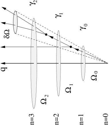
Figure 1: A schematic representation of the phase-space structure of branching inside jet. It makes use the angular ordering prescription: The structure of the cascade inside $\delta\Omega$ is determined by the “history” of this cascade inside the same $\delta\Omega$. Infinitesimal probabilities $W_{n}$ (not shown) control the structure of the cascade for full phase space $\Omega_{n}$. Local infinitesimal probabilities $\mathrm{\gamma}_{n}W_{n}$ determine the structure of cascade inside $\delta\Omega$.

We shall start our consideration with a simple two-dimensional model of a jet in angular intervals. Let us consider the first parton emitted at some angle with respect to the initial quark. Since we are interested in a picture averaged over all events, let $\Omega_{0}$ be the maximum possible size of solid angle, so that the first parton always has an angle inside the cone $\Omega_{0}$ (see Fig. 1). After its emission, the first parton radiates the next one at some angle with respect to its own direction of flight. Generally, we assume that there is recoil effect and the first parton can change its direction after this radiation. In this case, the solid angular window available for both partons becomes larger and is equal to $\Omega_{1}>\Omega_{0}$. The second parton then splits into two new partons at $\Omega_{2}$ and so on. One can further simplify the model taking into the account angular ordering when available phase space is reduced for successive branchings. In this case $\Omega_{0}\simeq\Omega_{1}\simeq\Omega_{2}\simeq\ldots\Omega_{n}$.

Let us tern to a more detailed description in one dimension. First, let us define $\Theta$ as the polar angle between the directions of motion of the emitted and the parent parton. The single-particle distribution $\rho(\Theta)$ of the gluon bremsstrahlung can be approximated [2, 3] at small $\Theta$ by

$$\rho(\Theta)=C(Q_{0},\alpha_{s})\Theta^{-1},$$ (22)

integrating the overall distribution over the azimuthal angle around the quark direction and momentum dependence. The $\Theta$-independent constant $C(Q_{0},\alpha_{s})$ contains a transverse momentum cut-off $Q_{0}$ and $\alpha_{s}$ which is treated here as a constant. The probability $\mathrm{\gamma}_{0}(\delta\Theta)$ of finding the gluon inside the small interval $(\Theta_{0}-\delta\Theta,\Theta_{0})$ near a jet opening angle $\Theta_{0}$ is

$$\mathrm{\gamma}_{0}(\delta\Theta)\propto\int_{\Theta_{0}-\delta\Theta}^{\Theta_{0}}\rho(\Theta)\mbox{d}\Theta\sim\delta\Theta^{\mathcal{D}_{0}},\quad\mathcal{D}_{0}=1$$ (23)

for $\delta\Theta\to 0$. Note that this result does not depend essentially on the details of the density $\rho(\Theta)$, since it has no singularity near $\Theta_{0}$. We did not specify a coefficient of proportionality between $\mathrm{\gamma}_{0}(\delta\Theta)$ and $\delta\Theta^{\mathcal{D}_{0}}$: As we have seen before, the phase-space dependence of the fluctuations does not depend on it.

Now let us consider the behavior of $\mathrm{\gamma}_{1}(\Theta)$ for the second parton. Since we are interested in the probability of emission of this parton into $(\Theta_{0}-\delta\Theta,\Theta_{0})$ under the condition that the first parton is inside the same interval, there is a larger probability of hitting this interval by the second parton because of the collinear singularity. Now the major problems in the calculating $\mathrm{\gamma}_{1}(\Theta)$ are: 1) An ambiguity in the position of the first parton inside $\delta\Theta$; 2) Singularity of $\rho(\Theta)$ near $\Theta\sim 0$ gives a dominant contribution. This leads to a very inhomogeneous phase-space distribution near $\Theta_{0}$; 3) Requirement of the angular ordering.

Due to the reasons quoted above, the calculation of $\mathrm{\gamma}_{n}(\Theta)$ for $n>1$ is even more difficult. We shall make no attempts to calculate $\mathrm{\gamma}_{n}(\Theta)$. In a general case, for small $\delta$, we assume

$$\mathrm{\gamma}_{n}(\delta\Theta)\propto\delta\Theta^{\mathcal{D}_{n}},\qquad n\geq 1,$$ (24)

where $\mathcal{D}_{n}$ are $\delta\Theta$-independent constants controlling the collinear singularities together with the angular ordering restrictions of the phase space available for particles on $(n+1)$th multiplicity stage. The latter effect decreases the available phase space for the next soft offspring partons that would increase the probability of detecting them inside $\delta\Theta$. We assume,

$$\mathcal{D}_{0}\geq\mathcal{D}_{1}\geq\mathcal{D}_{2}\geq\ldots\geq\mathcal{D}_{\infty}.$$ (25)

In subsection 3.2 we shall give an interpretation of the behavior (24) and (25) in terms of fractal distributions. Then we shall see that the behavior of $\mathrm{\gamma}_{n}(\delta\Theta)$ for small $\delta\Theta$ is the only simplest choice which allows to describe experimental data. In Sect. 4 we shall proceed with the physical interpretation of these quantities.

There are a number of special cases of interest:

1) Monofractal fluctuations

This case corresponds to the situation when the phase-space distributions for all cascade stages (except the initial one) have the same non-uniformity characterized by $\mathcal{D}_{1}$, i.e.,

$$\mathrm{\gamma}_{0}(\delta\Theta)\propto\delta\Theta^{\mathcal{D}_{0}},\qquad\mathrm{\gamma}_{n>0}(\delta\Theta)\propto\delta\Theta^{\mathcal{D}_{1}}.$$ (26)

Making use of (16), the BPs are

$$\eta_{2}(\delta\Theta)\propto\delta\Theta^{\mathcal{D}_{1}-\mathcal{D}_{0}},\qquad\eta_{q>2}(\delta\Theta)=const.$$ (27)

Hence, we obtain the monofractal behavior with $d_{2}=\mathcal{D}_{0}-\mathcal{D}_{1}$ [17, 18].

For cascade branchings, such a situation can be considered as a highly unrealistic since it totally disregards that daughter partons have ever larger probability to be emitted inside $\delta\Theta$ because of the correlations. Therefore, the monofractal type of intermittency possibly observed for some nucleus-nucleus reactions may mainly be attributed to other dynamical mechanisms [21], rather than to actual cascade processes with angular ordering.

2) Multifractal fluctuations

If particles on each cascade stage are distributed differently, then the cascade stage with the multiplicity $n+1$ should be characterized by its own $\mathcal{D}_{n}$, i.e.,

$$\mathrm{\gamma}_{n\geq 0}(\delta\Theta)\propto\delta\Theta^{\mathcal{D}_{n}}.$$ (28)

The corresponding BPs are

$$\eta_{q}(\delta\Theta)\propto\delta\Theta^{-\alpha_{q}},\qquad\alpha_{q}=\mathcal{D}_{q-2}-\mathcal{D}_{q-1}.$$ (29)

An inverse relation for $\mathcal{D}_{n}$ reads

$$\mathcal{D}_{n}=\mathcal{D}_{0}-\sum_{i=2}^{n+1}\alpha_{i}.$$ (30)

According to [17, 18], one has a multifractal behavior. An example of such a behavior will be given in subsection 3.4.

3.2 Connection with fractals

The simplicity of the model allows a natural connection of it with fractals. In this subsection we shall see that $\mathcal{D}_{n}$ introduced in (24) are nothing but fractal dimensions.

First, let us remind a standard definition of a fractal distribution. Let us assume that there is a large number $\mathcal{N}_{\mbox{tot}}$ of particles distributed over a phase space with the topological (Euclidean) integer dimension $D$ ($D=1,2,3$). Let $\mathcal{N}(\epsilon)$ be the number of particles counted inside the phase-space domain with a linear size $\epsilon$. The number $\mathcal{N}(\epsilon)$ and $\epsilon$ are related as

$$\mathcal{N}(\epsilon)\propto\epsilon^{\mathcal{D}},\qquad\epsilon\to 0,$$ (31)

where $\mathcal{D}$ is a fractal dimension, corresponding to the so-called box-counting (or mass, cluster $etc.$) dimension [23]. If the distribution is extremely inhomogeneous, $\mathcal{D}$ has a non-integer value ($\mathcal{D}<D$). If particles were uniformly distributed over the phase space, $\mathcal{D}$ is integer ($\mathcal{D}=D$). Therefore, $\mathcal{D}$ is a very economical way to describe the extent of non-uniformity of a distribution near a given small phase-space region.

It is easy to see that (31) also characterizes the probability $p$ of observing one particle inside $\epsilon$: This probability is determined by the ratio of the number $N(\epsilon)$ of events of observing a particle inside $\epsilon$ to the total number $N_{\mbox{tot}}$ of events. Assuming that only one particle can be emitted in each event, one has

$$p\equiv\frac{N(\epsilon)}{N_{\mbox{tot}}}=\frac{\mathcal{N}(\epsilon)}{\mathcal{N}_{\mbox{tot}}}\propto\epsilon^{\mathcal{D}},\qquad\epsilon\to 0.$$ (32)

Now let us tern to the model. In fact, the $\mathrm{\gamma}_{n}(\delta\Theta)$ has the same meaning as the $p$ defined in (32). The index $n$ in $\mathrm{\gamma}_{n}(\delta\Theta)$ simply specifies the cascade stage $n$ with the total $n+1$ particles, so that $\mathcal{D}_{n}$ stands the fractal dimension of the phase-space distribution of a single particle on each cascade stage. Then (23) describes a uniform particle distribution near $\Theta_{0}$ (no collinear singularity!). For the second particle, there is no such a uniformity any more: The collinear singularity of the emission of the second particle is near $\Theta_{0}$ and this leads to a very inhomogeneous distribution in this region, so that $\mathrm{\gamma}_{1}(\delta\Theta)\propto\delta\Theta^{\mathcal{D}_{1}}$, where $\mathcal{D}_{1}$ is a fractal dimension of this distribution ($\mathcal{D}_{1}<\mathcal{D}_{0}=1$). For the next emissions, the distribution should be even more inhomogeneous since parent particles are already non-uniformly distributed due to the collinear singularities and the angular ordering. Finally this leads to the condition $\mathcal{D}_{n}\geq\mathcal{D}_{n+1}$ guessed in (25).

The $\mathcal{D}_{n}$ are the usual fractal dimensions. However, after many cascade steps with different $\mathcal{D}_{n}$, one obtains a multifractal behavior (29) of the BPs. For a monofractality (27), the phase-space distribution for each particle in the cascade has to be characterized by a single fractal dimension for all $n$, $\mathcal{D}_{0}\neq\mathcal{D}=\mathcal{D}_{1}=\mathcal{D}_{2}=\ldots$.

3.3 Connection with factorial-moment method

A widely used means to study local fluctuations is based on the calculation of the normalized factorial moments [24]:

$$F_{q}(\delta\Theta)=\frac{\langle n(n-1)\ldots(n-q+1)\rangle}{\langle n\rangle^{q}},$$ (33)

where $n$ is the number of particles inside a restricted phase-space interval $\delta\Theta$, $\langle\ldots\rangle$ is the average over all events. For non-statistical fluctuations, $F_{q}(\delta\Theta)$ depend on the size of the phase-space interval $\delta\Theta$ as $F_{q}(\delta\Theta)\sim\delta\Theta^{-\phi_{q}}$, where $\phi_{q}$ are intermittency indices.

If the size of phase space is asymptotically small, then the following approximate relation between the $F_{q}(\delta\Theta)$ and the BPs holds [17, 18]:

$$F_{q}(\delta\Theta)\simeq\prod_{n=2}^{q}\eta_{n}^{q+1-n}(\delta\Theta).$$ (34)

From (34) and (29), one has

$$F_{q}(\delta\Theta)\propto\delta\Theta^{-\phi_{q}},\qquad\phi_{q}=\sum_{n=2}^{q}(q-n+1)\alpha_{n},$$ (35)

or, taking into account the expression for $\alpha_{n}$,

$$\phi_{q}=\sum_{n=2}^{q}(q-n+1)\,(\mathcal{D}_{n-2}-\mathcal{D}_{n-1}).$$ (36)

The case of no dynamical correlation corresponds to $\phi_{q}=0$. From (36), it follows that the only possibility for this case is the condition

$$\mathcal{D}_{0}=1=\mathcal{D}_{1}=\mathcal{D}_{2}=\ldots.$$ (37)

i.e., the next emitted partons are distributed over available phase space purely randomly (uniformly).

The model allows a simple way to connect the Rényi fractal dimension (see details in [7]) for factorial moments with the usual fractal dimensions $\mathcal{D}_{q}$ in our model. The Rényi fractal dimension $D_{q}$ is defined via $\phi_{q}$,

$$D_{q}=D-\frac{\phi_{q}}{q-1}.$$ (38)

From (36) one has,

$$D_{q}=\mathcal{D}_{1}-\sum^{q}_{n=3}\frac{q-n+1}{q-1}(\mathcal{D}_{n-2}-\mathcal{D}_{n-1}),$$ (39)

where we take into account that the topological dimension $D$ is equal to $\mathcal{D}_{0}$. From here one can again see that the monofractality ($D_{q}=const$) is possible only if $\mathcal{D}_{n-1}=\mathcal{D}_{n}$, for $n>1$. A variation of $D_{q}$ with $q$ for the multifractal case can be due to $\mathcal{D}_{n-1}\neq\mathcal{D}_{n}$.

In fact, the information about the fractal dimensions $\mathcal{D}_{n}$ can be extracted from the study of both $D_{q}$ (for factorial moments) or $\alpha_{q}$ (for bunching parameters). However, the study of the BPs is the most direct way to obtain the information on $\mathcal{D}_{n}$:

1) In contrast to the BPs, the power-like behavior of the normalized factorial moments holds only approximately for one dimensional variables because of a saturation effect for small rapidity intervals (see [6, 7, 12]).

2) The BP $\eta_{q}$ of order $q$ is a differential tool, resolving only the difference $\mathcal{D}_{q-2}-\mathcal{D}_{q-1}$ between the fractal dimensions $\mathcal{D}_{n}$ (see (29)). In contrast, the normalized factorial moment $F_{q}$ of order $q$ is an “integral” tool, which is sensitive to to all $\mathcal{D}_{n}$ with $n-1<q$. Because of the factor in the sum (39), the contribution from $\mathcal{D}_{n}$ at small $n$ is the largest. Hence, small changes in the behavior of $\mathcal{D}_{n}$ for large $n$ may be hidden due to contributions from $\mathcal{D}_{n}$ for small $n$.

3.4 Experimental data

The multifractal behavior (29) of BPs is characteristic for many different reactions [17]. For example, for rapidity variable with respect to the trust axis, BPs depend on the size of rapidity interval $\delta y$ as

$$\eta_{q}(\delta y)=\beta_{q}^{{}^{\prime}}\,\delta y^{-\alpha_{q}},\qquad q\geq 2,$$ (40)

where $\beta_{q}^{{}^{\prime}}$ and $\alpha_{q}$ are positive constants. This can be considered as an evidence that local fluctuations have a scale-invariant structure, $\eta_{q}(\lambda\delta y)=\lambda^{-\alpha_{q}}\eta_{q}(\delta y)$, i.e. the behavior is invariant under change of scale.

Usually, the power law (40) is represented in terms of the number $M=Y/\delta y$ of bins of size $\delta y$ covering a full phase-space volume $Y$, so that (40) becomes

$$\eta_{q}(M)=\beta_{q}^{{}^{\prime}}\,M^{\alpha_{q}}.$$ (41)

Taking the logarithm from both sides, the power law can be written as the linear expression

$$\ln\eta_{q}(M)=\alpha_{q}\ln M+\beta_{q},\qquad\beta_{q}=\ln\beta_{q}^{\prime}.$$ (42)

For $\mbox{e}^{+}\mbox{e}^{-}$ annihilations, such a behavior has been observed for rapidity defined with respect to the thrust axis (see Fig. 2 and [12, 17, 18]). That the $\alpha_{q}$ are not zero and vary with $q$ is a direct indication that the fluctuations in $y$ are multifractal. Table 2 shows the values of $\alpha_{q}$ and $\beta_{q}$ obtained using a fit by (42). To avoid trivial effects due to a bell-shaped structure of the multiplicity distribution at large $M$, the fit is limited to $\ln M>3$ for $q=2$ and $\ln M>2$ for $q>2$.

Fig. 3 and Table 2 show the predictions of the JETSET 7.4 PS [13] model with the L3 default parameters [22]. The charged final-state hadrons were generated at 91.2 GeV. The total number of events is 2.0M. The regions $\ln M<3$ (for $\eta_{2}$ and $\eta_{3}$) and $\ln M<2$ (for $\eta_{4}$) were excluded from the fits. Note also that $\chi^{2}$ test for the Monte Carlo is rather poor since, for the large statistics used, the behavior of $\eta_{q}(M)$ shows a clear complex structure caused by the presence of resonance decay products and the points for different $M$ are not statistically independent.

Table 2 shows the fractal dimensions $\mathcal{D}_{n}$ obtained using (29). The values of $\mathcal{D}_{n}$ decrease with increasing $n$, indicating that the degree of non-homogeneity of the distributions increases for particles emitted in the cascade later.

4 Model predictions

We have now set up a formalism that handles the local scale-invariant fluctuations inside a cascade. Qualitatively, the model proposed above can reproduce the power-like dependence of BPs observed in $\mbox{e}^{+}\mbox{e}^{-}$ data [12] and other process [17].

A most direct prediction of this approach is that the power-like behavior of the BPs is energy independent: The local fluctuations are determined by $\mathrm{\gamma}_{n}(\delta)$ in (18). They, in turn, depend only on the fractal dimensions $\mathcal{D}_{n}$. As a result, parameters $\alpha_{q}$ determining the phase-space fluctuations in (29) are $t$-independent.

The model, however, has only low predictive power unless we reduce the number of free parameters $\mathcal{D}_{n}$ in (29). To do this, let us rewrite the $\mathcal{D}_{n}$ as

$$\mathcal{D}_{n}=\mathcal{D}_{0}-A_{n},$$ (43)

so that positive $A_{n}$ represents the deviation of fluctuations from the trivial ones ($A_{n}=0$ actually corresponds to the case of no correlations or uniform cascade distributions). We shall call the parameters $A_{n}$ as the strength of dynamical correlations on the $n+1$ multiplicity stage of the branching. Since $\mathcal{D}_{n-1}\geq\mathcal{D}_{n}$, we have

$$A_{0}=0\leq A_{1}\leq A_{2}\leq\ldots\leq A_{n}.$$ (44)

The physical meaning of $A_{n}$ is rather clear: $A_{n}$ is determined by the collinear singularities of gluon emission and the extent of interference between soft partons leading to angular ordering. Generally, however, $A_{n}$ may absorb many other physical effects in jet beyond DLLA. This quantity can incorporate effects from energy-momentum balance (recoil effect) in two-parton splittings, heavy quark production and non-perturbative effects: hadronization, resonance decay and Bose-Einstein correlations. Since contributions from these effects are poorly known and at present cannot be taken into account in analytical calculations, below we shall make an attempt to treat $A_{n}$ on a general statistical ground.

Several remarkable features of $A_{n}$ are immediately apparent:

a) $A_{n}$ characterizes a single particle inside $\delta\Theta$ belonging to a system with $n$ other particles already produced inside this interval at the previous cascade stages.

b) Since $A_{n}$ is connected with correlations/fluctuations, one can consider it as a strength of “interaction” of a single particle with another. According to (44), such an interaction becomes stronger with the increase of multiplicity $n$.

These two features suggest that $A_{n}$ is analogous to the binding (pairing) energy per nucleon in nuclear physics. Using this analogy, the form of $A_{n}$ can be readily deduced without detailed information on correlations.

Let us first consider the following two extreme cases:

1) Since the Markov chain is based on two-particle splittings, one can assume that there exist positive correlations only between the particles $a_{1}$ and $a_{2}$ of the two-particle splitting $a_{1}\to a_{1}+a_{2}$, which is a basic element of the Markov chain. From a statistical point of view, the effect tends to make two partons more strongly bound in phase space, i.e., the probability that particles $a_{1}$ and $a_{2}$ occupy a very small phase-space bin is larger than that without dynamical correlations. After the next splitting of each particle, one has 2 two-particle pairs. For an $(n+1)$-particle system, the number of pairs stemming from the two-particle splittings is $(n+1)/2$, and we can write

$$A_{n}=A^{\mathrm{T}}\frac{n+1}{2},$$ (45)

where $A^{\mathrm{T}}$ is a constant describing the pair correlation in the case of two-particle correlations. Note that the applicability of (45) for odd $n$ is only an approximation to make the correlations easy to handle. We shall correct this expression later.

If only two-particle correlations (45) exist, then one obtains from (43) and (29)

$$\mathcal{D}_{n}=\mathcal{D}_{0}-A^{\mathrm{T}}\frac{n+1}{2},$$ (46)

$$\alpha_{2}=A^{\mathrm{T}},\qquad\alpha_{q\geq 3}=0.5\,A^{\mathrm{T}}.$$ (47)

The behavior $\alpha_{q}=0.5\alpha_{2}$ has been found to correspond to multiplicity fluctuations in $\mbox{p}\bar{\mbox{p}}$ collisions [17]. However, $\mbox{e}^{+}\mbox{e}^{-}$ data show a stronger multifractal signal. The behavior of (46) with $A^{\mathrm{T}}$=0.016 for the $\mbox{e}^{+}\mbox{e}^{-}$ data is shown in Fig. 4 ($A^{\mathrm{T}}>0,A^{\mathrm{M}}=0$). The value of $A^{\mathrm{T}}$ is equal to $\alpha_{2}$ taken from the experimental data (see Table 2). The model fails to reproduce the $n$-dependence of $\mathcal{D}_{n}$ for data and JETSET model.

2) Now let us consider another limiting case of correlations. Let us assume that each particle of a given $(n+1)$th particle generation is attracted in equal extent by all of the other $n$ particles already produced. There are exactly $n(n+1)/2$ interactions between $n+1$ particles uniformly distributed over the small phase-space volume. (Such a uniformity must, of course, be treated as an average over all events.) Hence, the correlation strength is (see Fig. 5)

$$A_{n}=A^{\mathrm{M}}\,\frac{n(n+1)}{2},$$ (48)

where $A^{\mathrm{M}}$ is a constant characterizing the correlation between any two particles. It completely determines many-particle correlations in such a system.

Having made this simple assumption, one has

$$\mathcal{D}_{n}=\mathcal{D}_{0}-A^{\mathrm{M}}\frac{n(n+1)}{2},$$ (49)

and, according to (29), the power-law indices for the BPs in the form

$$\alpha_{2}=A^{\mathrm{M}},\qquad\alpha_{q\geq 3}=A^{\mathrm{M}}(q-1).$$ (50)

The result for $A^{\mathrm{M}}=0.016$ is shown in Fig. 4 ($A^{\mathrm{T}}=0$, $A^{\mathrm{M}}>0$). As we see, this prediction is rather close to the experimental result. However, it still cannot give a satisfactory description of the data and JETSET model. In fact, such a disagreement is not a surprise since we systematically ignored the trivial fact that particles can interact with different strength.

As was mentioned, to some extent, $A_{n}$ is analogous to the binding (pairing) energy per nucleon in nuclear physics. In fact, expression (45) is analogous to the “volume” effect if the nuclear density is roughly constant. Then each nucleon has about the same number of neighbors and (45) actually represents the short-range correlations. Then (48) is analogous to the Coulomb repulsion term in the Weizsäcker mass formula which is proportional to [25]

$$-\alpha\frac{Z(Z-1)}{2},$$ (51)

where $Z$ is the number of protons and $\alpha=e^{2}/4\pi$ is the fine-structure constant of QED. The negative sign implies a reduction in binding energy. For QCD, of course, the Coulomb interaction is not the dominant part of the correlations and the introduced correlations should be attributed to other reasons.

Following the same logic, $A_{n}$ can be constructed analogously to the semi-empirical Weizsäcker mass formula by combining the different types of correlations and taking into account the obvious properties of the particle system in question. To see this, let us consider the following cascade chain:

$$a_{1}\to(a_{1}+a_{2})\to(a_{1}+a_{3})+a_{2}\to\ldots,$$

where the $a_{n}$ represents a parton in independent sequential splittings. The particles in parentheses are pairs arising due to two-particle splitting of parent particles on each stage. It is natural to assume that correlations between particles in the parentheses are different from those between the particles that have already been produced. For example, the particles in the pairs $(a_{1},a_{2})$ and $(a_{2},a_{3})$ produced on the three-particle stage can also be correlated, but to an extent different from those in the pair $(a_{1},a_{3})$ which stem directly from the two-particle splitting. Thus to make a step towards a more realistic description, it is necessary to take into account a non-homogeneity of parton interactions in the cascade.

First of all, let us describe the correlations between the particles in two-particle splittings. For this, we should take into account the odd-even effect in the two-particle correlations which is important for small $n$ (this was dropped for simplicity in (45)). A corrected expression (45) reads as

$$A^{\mathrm{T}}_{n}\equiv A^{\mathrm{T}}\times\left\{\begin{array}[]{ll}(n+1)/2,&\mbox{for $n=1,3,5,\ldots$}\\ n/2,&\mbox{for $n=2,4,6,\ldots$}\end{array}\right.$$ (52)

The next step is to take into account the multiparticle correlations arising between the particles produced in the previous stages of the cascade. As before, to simplify our considerations, we assume that this kind of (multiparticle) correlations can be characterized by a single parameter $A^{\mathrm{M}}$ responsible for the correlation between any particles stemming from different parents. For any $n$-particle system, the form of these correlations can be obtained by subtracting from a term of the form (48), representing all possible pair correlations, a term like (52) describing two-particle correlations which are taken into account by (52). The final expression reads

$$A^{\mathrm{M}}_{n}\equiv A^{\mathrm{M}}\frac{n(n+1)}{2}-A^{\mathrm{M}}\times\left\{\begin{array}[]{ll}(n+1)/2,&\mbox{for $n=1,3,5,\ldots$}\\ n/2,&\mbox{for $n=2,4,6,\ldots$}\end{array}\right.$$ (53)

The last step is to combine both contributions together,

$$\mathcal{D}_{n}=\mathcal{D}_{0}-A^{\mathrm{T}}_{n}-A^{\mathrm{M}}_{n},$$ (54)

$$\alpha_{2}=A^{\mathrm{T}},\qquad\alpha_{q\geq 3}=A^{\mathrm{T}}_{q-1}+A^{\mathrm{M}}_{q-1}-A^{\mathrm{T}}_{q-2}-A^{\mathrm{M}}_{q-2}.$$ (55)

Expressions (52), (53), (54) and (55) explicitly describe the behavior of the correlations in the cascade on the basis of the two parameters $A^{\mathrm{T}}$ and $A^{\mathrm{M}}$. The parameter $A^{\mathrm{T}}$ describes the correlation between particles stemming from the same parent particle and $A^{\mathrm{M}}$ characterizes the correlation between the particles coming from different parents. As in nuclear physics, we allow these constants to be adjustable and consider $A^{\mathrm{T}}$ and $A^{\mathrm{M}}$ as free parameters which can be evaluated from the fit.

The parameters $A^{\mathrm{M}}$ and $A^{\mathrm{T}}$ can be obtained from the two experimental parameters $\alpha_{2}^{\mbox{exp}}$ and $\alpha_{3}^{\mbox{exp}}$ describing the power-law behavior of BPs:

$$A^{\mathrm{T}}=\alpha_{2}^{\mbox{exp}},$$ (56)

$$A^{\mathrm{M}}=\alpha_{3}^{\mbox{exp}}/2.$$ (57)

Further evolution of the $\mathcal{D}_{n}$ and the $\alpha_{q}$ can be predicted by the model according to (54) and (55). For the $\mbox{e}^{+}\mbox{e}^{-}$ data presented in Table 2, one obtains $A^{\mathrm{T}}=0.016\pm 0.004$ and $A^{\mathrm{M}}=0.021\pm 0.002$. The predictions for $\mathcal{D}_{n}$ are shown in Fig. 4 ($A^{\mathrm{T}},A^{\mathrm{M}}>0$). The dashed lines show the uncertainty in the behavior of $\mathcal{D}_{n}$ due to the statistical errors on $A^{\mathrm{T}}$ and $A^{\mathrm{M}}$. Our predictions agree with the experimental data well. The agreement with the JETSET becomes better if one uses the values of $\alpha_{2}$ and $\alpha_{3}$ from the Monte-Carlo model to determine $A^{\mathrm{T}}$ and $A^{\mathrm{M}}$.

Note that expressions (54) and (55) cannot be valid for asymptotically large $n$ since the fractal dimensions $\mathcal{D}_{n}$ cannot be smaller then zero.

5 Discussion of the model predictions

One of the striking features of the results obtained is that good agreement between the model and the data is possible only if the value of $A^{\mathrm{T}}$ is smaller than that of $A^{\mathrm{M}}$. This means that the binding effect between two particles from the same parent must be smaller than that between particles produced earlier from different parent particles, i.e., the particles originating from different parents have a larger chance of being emitted very close to each other.

There are a number of possible explanations for this effect. If one believes that the model describes the perturbative QCD cascade, the reason for this may come directly from the color coherence effects. Indeed, the fact that $A^{\mathrm{M}}>0$ can be due to the angular ordering: For a given cascade stage with multiplicity $n$, collective correlation effects should exist between each particle due to the angular ordering history of the previous stages. Then the smallness of $A^{\mathrm{T}}$ can be explained by recoil effects and the minimal value of the relative transverse momentum $k_{\bot}$ of decay products in the cascade evolution, in order to ensure that partons have enough time to radiate, in their turn, new offspring [1]. The latter effect leads to a restriction on the relative emission angels between the particles $a_{1}$ and $a_{2}$ in the two-particle splitting $a_{1}\to a_{1}+a_{2}$. From a statistical point of view, the effect tends to make the two partons less tightly bound in phase space, i.e., the probability that both $a_{1}$ and $a_{2}$ particles occupy a very small phase-space bin is less than that without the restriction on the angle. If the reason for the condition $A^{\mathrm{T}}<A^{\mathrm{M}}$ indeed comes from perturbative QCD, $A_{n}^{\mathrm{T}}$ has to be connected with the momentum transfer cut-off $Q_{0}$ that limits the relative $k_{\bot}$ and plays the role of an effective mass of a parton.

On the other hand, it is reasonable to think that the proposed formulation of the branching process is sufficiently general and can utilize non-perturbative effects as well. In fact, the branching can be attributed to a certain degree to hadronization and resonance decay. Then, the multiparticle correlations can arise due to the color exchange between the partons at the end of the perturbative regime of QCD branching, necessary for parton discoloration. Furthermore, if the partons are replaced by hadrons, the large multiparticle correlations can be attributed to Bose-Einstein interference between identical pions, since these particles are usually produced by different parent ones. Then the smallness of $A_{n}^{\mathrm{T}}$ can be explained by an anti-correlation trend between decay products of resonances.

Note also that the model can be used for various complex non-point-like processes. In this context, one can consider the evolution of the multiplicity distributions for clusters, fireballs, resonances etc., taking into account peculiar features of these processes and introducing additional (or other) correlation terms in (54).

6 Summary and conclusion

In this paper we developed a new concept of local scale-invariant fluctuations in branching processes. In contrast to the approaches based on many-particle QCD correlation functions [2, 3] and phenomenological continuous densities [24], we adopted a method based on single-particle probabilities (or single-particle probability densities) for each cascade stage. They are characterized by the fractal dimensions $\mathcal{D}_{n}$ determining a non-uniformity in phase-space distributions for each particle emitted into a small phase-space domain. Such an idea simplifies the picture of phase-space organization of particles inside the cascade and allows us to take into account the finiteness of the number of particles in the cascade (or finite energy), QCD color coherence effects and a heterogeneity of correlations between partons belonging to the different cascade generations.

The fractal dimensions $\mathcal{D}_{n}$ can be experimentally observed by calculating the BPs which resolve the difference $\mathcal{D}_{n-1}-\mathcal{D}_{n}$, according to (29). A less direct way to measure $\mathcal{D}_{n}$ can be performed from the study of the normalized factorial moments (see (36)).

The model suggests and makes experimentally accessible new physical quantities - pair correlation coefficients $A^{\mathrm{M}}$ and $A^{\mathrm{T}}$ determining $\mathcal{D}_{n}$. The fact that none of these parameters are zero is due to the collinear singularities of the emission probabilities of soft partons. However, the way how these parameters determine the directly observable $\mathcal{D}_{n}$ can be due to many reasons. In this paper we suggest such a relationship using a general statistical formalism, which, in terms of QCD, may absorb the details of coherence effects, high-order perturbative corrections, recoil effects and non-perturbative phenomena, i.e. all the effects which at present can be combined together only on the basis of Monte-Carlo simulations. We allow $A^{\mathrm{M}}$ and $A^{\mathrm{T}}$ to be adjustable that ultimately leads to good quantitative agreement with the local fluctuations in $\mbox{e}^{+}\mbox{e}^{-}$ processes.

The model predicts that the experimentally observable parameters $\mathcal{D}_{n}$ determining the scale-invariant behavior of BPs $\eta_{q}(\delta)$ are energy independent. In addition, they do not depend on details of Markov equation in the full phase space. Both features follow from the factorization scheme used to derive the local fluctuations from the classical Markov branching equation for jet evolution and the angular ordering scheme which helps to construct the local version of this equation. Therefore, to check this approach, precise data on the behavior of the BPs with energy are needed.

Another model prediction is a suppression of positive correlations between the off-spring particles, $A^{\mathrm{M}}>A^{\mathrm{T}}$, a feature which can directly be detected from the study of $q$-dependence of the BPs. This prediction is also model dependent and the next step would be to understand how this effect can be changed if one uses another physical motivated parameterizations.

In spite of its simplicity, the model describes the correlations between partons in branchings beyond the scope of the Leading Log Approximation of QCD. To leading order in $\ln Q^{2}$, partons are free elementary quanta. Evidently, this situation corresponds to the particular case $\mathcal{D}_{n}=1$ (for all $n$) in our scheme. Since the model is constructed on the basis of angular ordering, it takes advantage of the DLLA. However, for very small $\delta$, the perturbative QCD ceases to be valid, since $Q_{0}$ sets the limit of validity of the smallest bin size and perturbative expansion of QCD. Hence, dealing with very small phase-space intervals, our model goes beyond the perturbative QCD approximations studied in [2]. At the same time, the model can take into account non-perturbative effects which are important if one goes beyond single-particle densities. It is evident that the price to pay for this progress in the description of multiparticle correlations inside jet is a purely statistical formalism eliminating the momentum dependence.

Acknowledgments

This work was started during my stay at the High Energy Physics Institute Nijmegen (HEFIN, The Netherlands). I thank W.Kittel for reading a first preliminary draft of this manuscript and for suggesting improvements.

$$\begin{array}[]{|l|c|c|c|c|c|c|}\hline\cr&\alpha_{q}&\beta_{q}&\chi^{2}/$df$&\alpha_{q}&\beta_{q}&\chi^{2}/$df$\\ \hline\cr\hline\cr&\lx@intercol\hfil$data$\hfil\lx@intercol\vrule\lx@intercol&\lx@intercol\hfil$JETSET 7.4 PS$\hfil\lx@intercol\vrule\lx@intercol\\ \hline\cr q=2&0.016\pm 0.004&0.244\pm 0.018&0.8/8&0.0206\pm 0.0005&0.224\pm 0.002&2.4/11\\ q=3&0.042\pm 0.003&0.08\pm 0.01&8/12&0.0434\pm 0.0007&0.075\pm 0.003&22/13\\ q=4&0.062\pm 0.004&0.01\pm 0.01&9/12&0.068\pm 0.001&-0.016\pm 0.004&36/10\\ q=5&0.071\pm 0.008&-0.03\pm 0.02&14/11&0.081\pm 0.002&-0.049\pm 0.004&91/10\\ q=6&-&-&-&0.072\pm 0.002&-0.019\pm 0.005&48/10\\ q=7&-&-&-&0.088\pm 0.003&-0.053\pm 0.006&64/8\\ \hline\cr\end{array}$$

Table 1: Fit results for $\eta_{q}(M)$ obtained from the $\mbox{e}^{+}\mbox{e}^{-}$ data [12]. The linear function (42) is used.

$$\begin{array}[]{|l|c|c|}\hline\cr&$data$&$JETSET 7.4 PS$\\ \hline\cr\hline\cr n=0&1.0&1.0\\ n=1&0.984\pm 0.004&0.9794\pm 0.0005\\ n=2&0.942\pm 0.005&0.936\pm 0.001\\ n=3&0.888\pm 0.006&0.868\pm 0.001\\ n=4&0.81\pm 0.01&0.787\pm 0.002\\ n=5&-&0.715\pm 0.003\\ n=6&-&0.627\pm 0.004\\ \hline\cr\end{array}$$

Table 2: The values of fractal dimensions $\mathcal{D}_{n}$ obtained from the experimental data and JETSET 7.4 PS. (see (30) and Table 2).

Figure 2: BPs for rapidity defined with respect to the thrust axis for $\mbox{e}^{+}\mbox{e}^{-}$ processes. Here $M=Y/\delta y$, where $Y$ is the size of full rapidity interval, $\delta y$ is the restricted rapidity interval. The data are reproduced from [12]. The lines represent the fit by (42) with the parameters presented in Table 2.

Figure 3: BPs for rapidity defined with respect to the thrust axis for JETSET 7.4 PS model. The lines show the fit by (42) with the parameters presented in Table 2.

Figure 4: The behavior of $\mathcal{D}_{n}$ for $\mbox{e}^{+}\mbox{e}^{-}$-annihilation data, JETSET 7.4 PS and the model predictions for: a) Two-particle correlations ($A^{\mathrm{T}}>0,A^{\mathrm{M}}=0$); b) Multiparticle correlations ($A^{\mathrm{T}}=0$, $A^{\mathrm{M}}>0$); c) Both two-particle and multiparticle correlations ($A^{\mathrm{T}},A^{\mathrm{M}}>0$).

Figure 5: A schematic representation of the multiparticle correlations for an $(n+1)$-particle system ($n=1,2,3$).

References

- [1] Yu.L.Dokshitzer, V.A.Khoze, A.H.Mueller, S.I.Troyan, Rev. Mod. Phys. 60, 375 (1988); Basics of Perturbative QCD, Editions Frontiers (Gif-sur-Yvette Cedex, France, 1991)
-
[2]
W.Ochs and J.Wosiek, Phys. Lett. B 289, 159 (1992);
W.Ochs and J.Wosiek, Phys. Lett. B 304, 144 (1993);
Yu.L.Dokshitzer and I.M.Dremin, Nucl. Phys. B 402, 139 (1993);
Ph. Brax, J.L. Meunier and R.Peschanski, Z. Phys. C 62, 649 (1994) -
[3]
W.Ochs and J.Wosiek, Z. Phys. C 68, 269 (1995);
V.A.Khoze and W.Ochs, Int. J. Mod. Phys. A 12, 2949 (1997) - [4] B.Buschbeck and F.Mandl (DELPHI Coll.), ICHEP’96 contributed paper pa01-028; B.Buschbeck, P.Lipa and F.Mandl (DELPHI Coll.), in Proc. 7th Int. Workshop on Multiparticle Correlations and Fluctuations, Nijmegen, The Netherlands 1996, Eds: R.C.Hwa et al. (World Scientific, Singapore, 1997) p.175;
- [5] L3 Coll., M. Acciarri et al., CERN-EP/98-23 (Phys. Lett. B, in press)
- [6] P.Bożek, M.Płoszajczak and R.Botet, Phys. Reports 252, 101 (1995)
- [7] E.A.De Wolf, I.M.Dremin and W.Kittel, Phys. Reports 270, 1 (1996)
-
[8]
K.Konishi, A.Ukawa and G.Veneziano, Nucl. Phys. B 157, 45 (1979);
P.Cvitanović, P.Hoyer, K.Zalewski, Nucl. Phys. B 176, 429 (1980) - [9] A.Giovannini, Nucl. Phys. B 161, 429 (1979)
- [10] M.Biyajima and N.Suzuki, Phys. Lett. B 143, 463 (1984); Prog.Theor. Phys. 73, 918 (1985)
-
[11]
B.Durand and I.Sarcevic, Phys. Rev. D 36, 2693 (1987);
I.Sarcevic, Phys. Rev. Lett. 59, 403 (1987);
I.Sarcevic, in Hadronic Matter in Collisions, Eds. P.Carruthers and J.Rafelski (World Scientific, Singapore, 1988) p.78 - [12] L3 Coll., M. Acciarri et al., CERN-PPE/97-165 (Phys. Lett. B, in press)
- [13] T.Sjöstrand, Computer Phys. Commun. 82, 74 (1994)
- [14] D.R.Cox and H.D.Miller, The Theory of Stochastic Processes, Chapman and Hall Ltd., London, 1972
- [15] A.Giovannini, S.Lupia and R.Ugoccioni, Phys. Lett. B 374, 231 (1996)
- [16] A.Giovannini, S.Lupia and R.Ugoccioni, Phys. Lett. B 388, 639 (1996)
- [17] S.V.Chekanov and V.I.Kuvshinov, Acta Phys. Pol. B 25, 1189 (1994)
-
[18]
S.V.Chekanov, W.Kittel and V.I.Kuvshinov, Acta Phys. Pol.
B 27, 1739 (1996);
S.V.Chekanov, W.Kittel and V.I.Kuvshinov, Z. Phys. C 73, 517 (1997) - [19] S.V.Chekanov and V.I.Kuvshinov, J. Phys. G 23, 951 (1997)
- [20] S.V.Chekanov and V.I.Kuvshinov, J. Phys. G 22, 601 (1996)
- [21] A.Białas and R.C.Hwa, Phys. Lett. B 253, 613 (1991)
- [22] L3 Coll., B. Adeva et al, Z.Phys. C 55, 39 (1992)
-
[23]
B.Mandelbrot, The Fractal Geometry of Nature,
W.H.Freeman and Co., San Francisco, 1982;
J.Feder, Fractals, Plenum Press, New York, 1988 - [24] A.Białas and R.Peschanski, Nucl. Phys. B 273, 703 (1986); Nucl. Phys. B 308, 859 (1988)
- [25] K.S.Krane, Introductory Nuclear Physics, John Wilew and Sons. Inc. 1987, p.56