Preprint MSU Faculty of Physics 7/98

Production of Higgs with Z–boson by an electron in external fields

P. A. Eminov

Department of Physics
Moscow State Institute of Electronics and Mathematics
(Technical University)
109028, Moscow, Russia
K. V. Zhukovskii, K. G. Levtchenko

Faculty of Physics,
Department of Theoretical Physics, Moscow State University,
119899, Moscow, Russia

The rate of associative production of Higgs and $Z$–bosons by charged leptons in the field of a plane electromagnetic wave of arbitrary intensity and in the constant crossed field is obtained. The cross section is examined as a function of particle energies and external field intensities for various values of the Higgs boson mass. It is shown, that the photoproduction cross section increases logarithmically at super high energies up to the values, that essentially exceed the cross section of the reaction $e^{+}e^{-}\to ZH,$ which, at present, is considered as the most probable channel of Higgs boson production.

1 Introduction

The Higgs mechanism of spontaneous symmetry breaking is one of the key elements in the electroweak sector of the Standard Model, along with the principle of gauge invariance. It is due to this principle that fundamental particles, quarks and weak gauge bosons, acquire masses through their interaction with a scalar Higgs field.

At present, the fundamental massive Higgs boson is the only particle of the Standard Model which has not been observed so far. Experimental discovery of the scalar Higgs bosons could provide an important test of the Standard Model and even of the Higgs mechanism of spontaneous symmetry breaking in particle physics itself.

According to the Weinberg–Salam–Glashow (WSG) theory the masses of the $W^{\pm}$– and $Z$–bosons as well as the vacuum expectation value $v$ of the Higgs field can be written in terms of the Fermi constant $G_{F}$, the fine structure constant $\alpha,$ and the Weinberg angle $\theta_{W}$ [1, 2]:

$$M_{W}=\left(\frac{\displaystyle\pi\alpha}{\displaystyle\sqrt{2}G_{F}}\right)^{1/2}\frac{\displaystyle 1}{\displaystyle\sin\theta_{W}}=80,37\pm 0,19\,Gev,$$

$$M_{Z}=\frac{\displaystyle M_{W}}{\displaystyle\cos\theta_{W}}=91186,3\pm 1,9\,Mev,\;v=(\sqrt{2}G_{F})^{-1/2}\simeq 246\,Gev.$$

The vacuum expectation value $v$ and the weak mixing angle $\theta$ are experimentally determined, so that the only unknown parameter is the mass of the Higgs particle:

$$M_{H}=\lambda v,$$

which depends on the as yet unknown Higgs boson self–coupling constant $\lambda.$

Since in the WSG theory couplings of Higgs bosons to other particles grow with the masses of these particles, interactions of Higgs bosons with gauge bosons and heavy quarks are much stronger than those with electrons and other light particles. Therefore processes of associative production of Higgs particles with gauge $W^{\pm}$– and $Z$–bosons are considered to be the most effective ones in the entire range of possible Higgs production mechanisms and are of substantial theoretical and practical interest.

The main Higgs particle production mechanisms in $e^{+}e^{-}$–collisions are the Higgs strahlung off the $Z$–boson line $e^{+}+e^{-}\to Z\to Z+H$ and the fusion processes $e^{+}+e^{-}\to W^{+}W^{-}\nu_{e}\tilde{\nu}_{e}\to H+\nu_{e}+\tilde{\nu}_{e},$ $e^{+}+e^{-}\to e^{+}e^{-}ZZ\to e^{+}+e^{-}+H$ [3–6], among which the $e^{+}+e^{-}\to Z+H$ process dominates at $\sqrt{s}\mathbin{\mbox{\am\char 46\relax}}500\,$GeV [7], where $\sqrt{s}$ is the c.m. energy of colliding particles. The direct search for the process $e^{+}+e^{-}\to Z+H$ at LEP2 sets a lower bound for the Higgs mass of $M_{H}>75$ GeV [1]. In this case the cross section does not exceed $0.3\,$pb for the Higgs boson mass $M_{H}\in(50,350)$ GeV, and it decreases at higher values of $M_{H}$.

Taking into account the direct measurements of $t$–quark and $W$–boson masses at Tevatron, the mass of the Higgs particle is considered to be $\displaystyle 127^{+127}_{-72}$ GeV, and at a confidence level of 95 % it must be less than $465$ GeV [1].

As for the upper limit for the $H$–boson mass in the Standard Model, it can be derived from the estimation of the energy range within which the model is assumed to be valid, i.e., before the particles interaction becomes strong. Taking into account that the strength of the Higgs self–interaction as well as of the interaction of $W$– and $Z$–bosons with Higgs particle is determined by the Higgs mass and the constant $\lambda$, we obtain that at $M_{H}\gg M_{Z},$ $M_{H}\gg M_{W}$ interaction between particles appears to be strong. The detailed analysis leads to an estimate of about 700 GeV for the upper limit of $M_{H}$ [7–10].

Electron–photon collisions are among other possible channels of Higgs boson production. For example, the dependence of the cross section of the process $e+\gamma\to W+H+\nu_{e}$ upon the mass of the Higgs boson for the energy range $\sqrt{s}=200\div 2000$ GeV is studied in [11, 12] and as it was shown in [12], production of Higgs bosons with mass values greater than 140 GeV in the reaction $e+\gamma\to e\gamma\gamma\to e+H,$ is quite feasable for $\sqrt{s}>500$ GeV. To produce hard photons in this case the inverse Compton effect can be used with a nearly monochromatic spectrum of scattered photons for $\chi=\frac{\displaystyle 2\omega E}{\displaystyle m^{2}}\gg 1$, having a sharp maximum at $\omega^{\prime}\approx E$. Here $\omega,$ $\omega^{\prime},$ $E$ are the energies of the incident and scattered photons, and of the relativistic electron respectively.

The Higgs bosons production and decay processes in the presence of external electromagnetic fields are actually of great interest. The importance of these studies are determined by the fact that in the field of an external electromagnetic wave the rates of many processes, that are usually forbidden by the 4-momentum conservation law, increase substantially, reaching measurable values, and, on the other hand, many reactions become more informative in the presence of external electromagnetic fields [13–15].

In the present paper the associative production of Higgs and $Z$–bosons by a charged lepton in external electromagnetic fields of various configurations is examined. The rates are calculated with the use of the relativistic wave functions of the particles in the external field which enables interactions of charged particles with external electromagnetic field to be considered exactly [13–16].

In Section 2 the rate of the process $e\to e+Z+H$ in the presence of the electromagnetic wave field of arbitrary intensity and configuration is calculated.

In Section 3 the crossed field case is examined. Under the condition, that the electron is extremely relativistic and the intensity of the field is relatively small ($E,\,H\ll H_{0}=\frac{\displaystyle m^{2}}{\displaystyle e}\simeq 4,41\cdot 10^{13}$ Gs), the results obtained can be applied to the case of an arbitrary constant field.

In Section 4 the asymptotics for the Higgs boson production rate in the cases of the crossed field and an electromagnetic wave are obtained. It is shown that the Higgs production cross section in the reaction $e+\gamma\to e+Z+H$ with photons absorbed from the wave and with high energy electrons can exceed the rate of the reaction $e^{-}+e^{+}\to Z+H$, which is considered to be one of the most probable channel of Higgs production [1, 3, 4].

2 Process $e\to e+Z+H$ in the presence of an external electromagnetic wave.

In the Standard Model framework the matrix element of the process examined can be written as follows [17]

$$\langle f|S^{(2)}|i\rangle=\frac{\displaystyle ig^{2}M_{Z}}{\displaystyle\cos^{2}\Theta_{W}\sqrt{4k_{0}k^{\prime}_{0}}}J^{\mu}\left[g_{\mu\nu}-\frac{\displaystyle p_{\mu}p_{\nu}}{\displaystyle M^{2}_{Z}}\right]\frac{\displaystyle e^{(\lambda)*}_{\nu}(k^{\prime})}{\displaystyle p^{2}-M^{2}_{Z}+i\Gamma_{Z}M_{Z}},$$

where $\Gamma_{Z}\simeq 2494,7\pm 2,6$ MeV is the $Z$–boson decay width , $k=(k_{0},{\bf k}),$ $k^{\prime}=(k^{\prime}_{0},{\bf k^{\prime}}),$ $p$ are the momenta of the Higgs boson, outgoing $Z$–boson, and virtual $Z$–boson respectively, and

$$J^{\mu}=\int d^{4}x\bar{\psi}_{q^{\prime}}(x)\gamma^{\mu}(g_{V}+g_{A}\gamma^{5})\psi_{q}(x)\exp(ipx)$$

is the electroweak current. Here $g_{A}=-1/4,\;g_{V}=-1/4+\sin^{2}\Theta_{W}$ and $\psi_{q}(x)$ is the exact solution of the Dirac equation for an electron in the given external field.

The wave function of an electron in the field of an external plane electromagnetic wave described by the 4–potential $A^{\mu}=A^{\mu}(\varphi)$ (the phase $\varphi=nx$, where $n$ is a wave vector, $n^{2}=0$), is given by the following expression [14,18]:

$$\psi_{q}(x)=(2q_{0}V)^{-1/2}\left[1+\frac{\displaystyle e}{\displaystyle 2(nq)}(\gamma n)(\gamma A)\right]u(q)\exp(iS_{q}(x)).$$ (1)

Here $V$ is the normalization volume, and $u(q)$ is the bispinor amplitude of the free particle solution of the Dirac equation

$$(\gamma q-m)u(q)=0,\;\;q^{2}=m^{2},$$

and $S_{q}(x)$ coincides with the classical action for the particle, moving in the external plane wave field:

$$S_{q}(x)=-qx-\int\limits^{\varphi}_{0}d\varphi\left[\frac{\displaystyle e}{\displaystyle(nq)}(qA)-\frac{\displaystyle e^{2}A^{2}}{\displaystyle 2(nq)}\right].$$ (2)

In the case of a circularly polarized plane wave, determined by the potential

$$A^{\mu}(x)=a^{\mu}_{1}\cos\varphi+a^{\mu}_{2}\sin\varphi,$$

$$a^{2}_{1}=a^{2}_{2}=a^{2},\;a_{1}a_{2}=0,\;a_{1}n=a_{2}n=0,\;\varphi=nx,$$

the following expression for the wave function is obtained from (1) and (2):

$$\psi_{q}(x)=\left[1+\frac{\displaystyle e}{\displaystyle 2(nq)}(\hat{n}\hat{a}_{1}\cos\varphi+\hat{n}\hat{a}_{2}\sin\varphi)\right]\times$$

$$\times\frac{\displaystyle u(q)}{\displaystyle\sqrt{2Q_{0}}}\exp\left\{-ie\frac{\displaystyle a_{1}q}{\displaystyle nq}\sin\varphi+ie\frac{\displaystyle a_{2}q}{\displaystyle nq}\cos\varphi-iQx\right\}.$$

Here the electron momentum in the presence of an external plane wave field was introduced

$$Q^{\mu}=q^{\mu}-e^{2}\frac{\displaystyle a^{2}}{\displaystyle 2(nq)}n^{\mu},$$

whose square is equal to the electron effective mass in the presence of an external field:

$$Q^{2}=m^{2}_{*}=m^{2}(1+\xi^{2}).$$

In this expression $\xi=\sqrt{-\frac{\displaystyle e^{2}a^{2}}{\displaystyle m^{2}}}$ is the well known parameter of the wave intensity determined by the ratio of the work produced by the field in its wavelength to the electron energy at rest.

The averaging of the squared matrix element with respect to the spin states of initial electron and summing over polarizations of the outgoing electron is carried out according to the common procedure, while the sum over polarizations of the $Z$–boson is obtained with the use of the following formula:

$$\sum_{\lambda=1,2,3}e^{(\lambda)}_{\nu}(k^{\prime})e^{(\lambda)}_{\mu}(k^{\prime})=-\left(g_{\mu\nu}-\frac{\displaystyle k^{\prime}_{\mu}k^{\prime}_{\nu}}{\displaystyle M^{2}_{Z}}\right),$$

where $e^{(\lambda)}_{\nu}(k^{\prime})$ is the $Z$–boson polarization 4–vector.

Upon integrating, made in the tensor form, with respect to the Higgs and the outgoing $Z$–boson phase volumes the rate of the process in the unit space volume is obtained

$$W=\frac{\displaystyle G^{2}_{F}}{\displaystyle(2\pi)^{3}}M^{6}_{Z}\frac{\displaystyle m^{2}}{\displaystyle Q_{0}}\sum_{s>s_{0}}\int\limits^{u_{2}}_{u_{1}}\frac{\displaystyle du}{\displaystyle(1+u)^{2}}\int\limits^{\tau(u)}_{M^{2}}\frac{\displaystyle d\tau\sqrt{(\tau-M^{2}_{Z}-M^{2}_{H})^{2}-4M^{2}_{Z}M^{2}_{H}}}{\displaystyle\tau((\tau-M^{2}_{Z})^{2}+(\Gamma_{Z}M_{Z})^{2})}\times$$

$$\times\left\{AE-4g^{2}_{A}\frac{\displaystyle m^{2}}{\displaystyle M^{2}_{Z}}F\left(B\frac{\displaystyle(\tau-M^{2}_{Z})^{2}}{\displaystyle M^{4}_{Z}}+A\left(2-\frac{\displaystyle\tau}{\displaystyle M^{2}_{Z}}\right)\right)\right\},$$ (3)

$$E=(g^{2}_{A}+g^{2}_{V})\left[-2\xi^{2}\frac{\displaystyle u^{2}+2u+2}{\displaystyle u+1}(J^{2}_{s+1}+J^{2}_{s-1}-2J^{2}_{s})-\right.$$

$$\left.-8J^{2}_{s}\left(1-\frac{\displaystyle\tau}{\displaystyle 2m^{2}}\right)\right]+16(g^{2}_{V}-g^{2}_{A})J^{2}_{s}+$$ (4)

$$+2g_{A}g_{V}\frac{\displaystyle u+2}{\displaystyle u+1}J_{s}(J_{s-1}-J_{s+1})\frac{\displaystyle np}{\displaystyle m^{2}}4z\left(1-\frac{\displaystyle 2\xi^{2}}{\displaystyle 1+\xi^{2}}\frac{\displaystyle u}{\displaystyle u_{s}z^{2}}\right),u_{s}=\frac{\displaystyle 2s(np)}{\displaystyle m^{2}_{*}},$$

$$F=-2\frac{\displaystyle\tau}{\displaystyle m^{2}}J^{2}_{s}+\frac{\displaystyle u^{2}}{\displaystyle u+1}\xi^{2}(J^{2}_{s+1}+J^{2}_{s-1}-2J^{2}_{s}),\;\;M=M_{Z}+M_{H},$$

$$A=\frac{\displaystyle 8\tau M^{2}_{Z}+(\tau+M^{2}_{Z}-M^{2}_{H})^{2}}{\displaystyle 12\tau M^{2}_{Z}},\;\;B=\frac{\displaystyle(\tau+M^{2}_{Z}-M^{2}_{H})^{2}-\tau M^{2}_{Z}}{\displaystyle 3\tau^{2}}.$$

Each term in the series (3) corresponds to the Higgs and $Z$–bosons production accompanied by absorption of $s$ photons from the wave, with their minimal number being equal to

$$s_{0}=\frac{\displaystyle(M+m_{*})^{2}-m^{2}_{*}}{\displaystyle 2(nq)}.$$

In the expressions (3), (4) for the rate of the process the new variables $u=-1+\frac{\displaystyle(nq)}{\displaystyle(nq^{\prime})},$ $\tau=(sn+q-q^{\prime})^{2},$ and the boundaries

$$u_{1,2}=\frac{\displaystyle(sn+q)^{2}-M^{2}-m^{2}_{*}\pm\sqrt{((sn+q)^{2}-M^{2}-m^{2}_{*})^{2}-4m^{2}_{*}M^{2}}}{\displaystyle m^{2}_{*}},$$

$$\tau(u)=\frac{\displaystyle(sn+q)^{2}u}{\displaystyle 1+u}-m^{2}_{*}u.$$

were introduced.

The argument of the Bessel functions in the expression (4) for the rate is equal to

$$z=2s\frac{\displaystyle\xi}{\displaystyle\sqrt{1+\xi^{2}}}\sqrt{\frac{\displaystyle u}{\displaystyle u_{s}}\left(1-\frac{\displaystyle u}{\displaystyle u_{s}}-\frac{\displaystyle\tau(1+u)}{\displaystyle uu_{s}m^{2}_{*}}\right)}.$$

The result obtained (3), (4) is exact, i.e., it is valid for any value of the classical parameter of the wave intensity, the nonlinearity domain, $\xi^{2}\mathbin{\mbox{\am\char 38\relax}}1,$ including. In this region interaction of an electron with the intensive electromagnetic wave field leads to new effects, nonlinearly depending on the energy density of the wave.

Below a particular case, $\xi\ll 1,$ will be considered, when the perturbation theory can be applied and the processes with minimal number of absorbed photons are most probable. Upon representing (3), (4) as a power series in $\xi^{2},$ the following condition

$$2(nq)>(M+m_{*})^{2}-m^{2}_{*},$$ (5)

is to be satisfied, which means that the process with a single photon absorbed from the wave becomes possible.

Thus, dividing the rate (3) by the incident current density $j=\frac{\displaystyle m^{2}\ae}{\displaystyle 2\omega EV}$ ($\omega$ is the photon energy, $E$ is the electron energy, $\ae=\frac{\displaystyle 2(nq)}{\displaystyle m^{2}}$) and putting $\xi^{2}=\frac{\displaystyle 4\pi\alpha}{\displaystyle m^{2}\omega V}$ ($\alpha$ is the fine structure constant), the cross section of the process $e+\gamma\to e+Z+H$ is finally obtained

$$\sigma=\left(\frac{\displaystyle eG_{F}m}{\displaystyle\pi}\right)^{2}\left(\frac{\displaystyle M^{2}_{Z}}{\displaystyle\ae m^{2}}\right)^{2}\int\limits^{1-a}_{b}\frac{\displaystyle d\lambda(1-M^{2}/(\ae\lambda m^{2}))^{1/2}(1-M^{2}_{1}/(\ae\lambda m^{2}))^{1/2}}{\displaystyle(\lambda-M^{2}_{Z}/(\ae M^{2}))^{2}}\times$$

$$\times\left\{2AC-4g^{2}_{A}\frac{\displaystyle m^{2}}{\displaystyle M^{2}_{Z}}D\left[B\frac{\displaystyle m^{4}\ae^{2}}{\displaystyle M^{4}_{Z}}\left(\lambda-\frac{\displaystyle M^{2}_{Z}}{\displaystyle\ae m^{2}}\right)^{2}+A\left(2-\frac{\displaystyle\ae\lambda m^{2}}{\displaystyle M^{2}_{Z}}\right)\right]\right\},$$ (6)

where $\lambda=\frac{\displaystyle\tau}{\displaystyle m^{2}\ae},$

$$C=(g^{2}_{V}+g^{2}_{A})[2\lambda(1-\lambda)-1]\ln\frac{\displaystyle 1-\lambda}{\displaystyle a}-2\lambda(g^{2}_{V}+g^{2}_{A})(1-\lambda-a)+$$

$$+4g_{V}g_{A}\left(\frac{\displaystyle 1}{\displaystyle 2}-\lambda\right)\ln\frac{\displaystyle 1-\lambda}{\displaystyle a}-4g_{V}g_{A}(1-\lambda-a),\;\;M_{1}=M_{Z}-M_{H},$$

$$D=[1-2\lambda(1-\lambda)]\ln\frac{\displaystyle 1-\lambda}{\displaystyle a}+2\lambda(1-\lambda-a),\;\;b=\ae a=\frac{\displaystyle 1}{\displaystyle\ae}\frac{\displaystyle M^{2}}{\displaystyle m^{2}},$$

and $A,B$ are determined by (4).

3 $e\to e+Z+H$ process in the presence of a constant crossed field.

In the present section production of Higgs bosons in constant crossed fields with intensity vectors ${\bf E}$ and ${\bf H}$ normal and with their magnitudes equal $|{\bf E}|=|{\bf H}|$ to each other (this means that both of the field invariants are equal to zero) is considered.

This crossed field can be regarded as an exceptional limiting case of a plane wave electromagnetic field, determined by the vector potential

$$A^{\mu}=a^{\mu}\varphi,\;\;an=0.$$ (7)

Thus, with regard to (1) there follows an expression for the electron wave function in the crossed field

$$\psi_{q}(x)=\left[1+\frac{\displaystyle e(\gamma n)(\gamma a)}{\displaystyle 2(nq)}\varphi\right]\frac{\displaystyle u(q)}{\displaystyle\sqrt{2q_{0}V}}\times$$

$$\times\exp\left[-ie\frac{\displaystyle aq}{\displaystyle 2(nq)}\varphi^{2}+ie^{2}a^{2}\frac{\displaystyle\varphi^{3}}{\displaystyle 6(nq)}-iqx\right].$$

The rate of the process $e\to e+Z+H$ can be derived from (1) in a standard way after some computations with the use of the electron wave function in a crossed field, but here an alternative method for calculating the rate, based on the exact result (3) obtained for the case of a circulary polarized wave will be employed. Indeed, the total rate of the process $e\to e+Z+H$ in the presence of such a wave depends on the two invariant parameters

$$\xi=\sqrt{-\frac{\displaystyle e^{2}a^{2}}{\displaystyle m^{2}}}=\frac{\displaystyle eF}{\displaystyle m\omega},\;\;\chi=\frac{\displaystyle e}{\displaystyle m^{3}}[-(F^{\alpha\beta}q_{\beta})]^{1/2}=\xi\frac{\displaystyle(nq)}{\displaystyle m^{2}}.$$

Herewith the electric and magnetic field intensity vectors rotate in the plane normal to the direction of the wave propagation at the frequency equal to the frequency of the wave.

Thus, the total rate of the process, calculated in the presence of a plane wave with circle polarization for $\omega\to 0\;(\xi\to\infty)$ and that in a constant crossed field must be exactly equal [14, 15, 18]:

$$\lim_{\xi\to\infty}W(\xi,\chi)\equiv W(\infty,\chi)\equiv W(\chi).$$ (8)

It should be noted, that the result obtained in the limit (8) is valid for the crossed electromagnetic field at arbitrary value of the electron energy, and moreover, if $\varepsilon\gg m,$ (i.e. extremely relativistic case) it describes the rate of the process under consideration for an arbitrary configuration of a constant relatively weak electromagnetic field $F\ll H_{0}$ [14].

Next, the order of summing in the series and integrating in (3) are interchanged yielding the expression

$$W=\sum_{s>s_{0}}\int\limits^{2\pi}_{0}d\varphi\int\limits^{\infty}_{0}du\int\limits^{\infty}_{M^{2}}d\tau W(u,\tau,s,\varphi)=$$

$$=\int\limits^{2\pi}_{0}d\varphi\int\limits^{\infty}_{0}du\int\limits^{\infty}_{\left(\frac{M}{m}\right)^{2}}d\alpha\sum_{s>s_{min}}m^{2}W(u,\alpha,s,\varphi),$$

where

$$\alpha=\frac{\displaystyle\tau}{\displaystyle m^{2}},\;s_{min}=\frac{\displaystyle\xi^{3}u}{\displaystyle 2\chi}\left[1+\frac{\displaystyle 1}{\displaystyle\xi^{2}}\left(1+\alpha\frac{\displaystyle u+1}{\displaystyle u^{2}}\right)\right],\;\;\chi=\frac{\displaystyle nq}{\displaystyle m^{2}}\xi.$$

If $\xi^{2}\gg 1,$ the value of the rate of the process is determined by the region $z\sim s\sim\xi^{3}\gg 1,$ since it gives the dominant contribution to the result. Therefore, we can substitute summation over $s$ by integration with respect to a new variable $\tau$ using the following relations between s and $\tau$:

$$s=\frac{\displaystyle\xi^{3}u}{\displaystyle 2\chi}\left(1+\frac{\displaystyle 2\tau}{\displaystyle\xi}\right)+s_{min}.$$

The final result is

$$W=\int\limits^{2\pi}_{0}d\varphi\int\limits^{\infty}_{0}du\int\limits^{\infty}_{\left(\frac{M}{m}\right)^{2}}d\alpha\int\limits^{\infty}_{-\frac{\xi}{2}}d\tau\frac{\displaystyle\xi^{2}u}{\displaystyle\chi}m^{2}W(\varphi,u,\tau,\alpha).$$ (9)

For high values $\xi^{2}\gg 1$ the rate $W(\varphi,u,\tau,\alpha)$ can be representd using the following asymptotics [19] for the Bessel functions, which is valid when their argument and index tend to infinity, while their ratio tends to unity, :

$$J_{s}(z)\simeq\frac{\displaystyle 1}{\displaystyle\pi}\left(\frac{\displaystyle 2}{\displaystyle s}\right)^{1/3}\Phi(y),$$

where $\Phi(y)$ is the Airy function of the argument

$$y=\left(\frac{\displaystyle s}{\displaystyle 2}\right)^{2/3}\left(1-\frac{\displaystyle z^{2}}{\displaystyle s^{2}}\right)=\left(\frac{\displaystyle u}{\displaystyle 2\chi}\right)^{2/3}\left[1+\alpha\frac{\displaystyle u+1}{\displaystyle u^{2}}+\tau^{2}\right].$$

After the limiting procedure has been performed, integration in (9) with respect to the angular variable $\tau$ be can carried out taking into account the well known relations for the Airy functions, cited in [14]. Thus, the following representation for the total rate of the process $e\to e+Z+H$ in the presence of a crossed field is finally obtained

$$W=-\frac{\displaystyle 1}{\displaystyle\sqrt{\pi}}\frac{\displaystyle G^{2}_{F}M^{6}_{Z}}{\displaystyle(2\pi)^{3}Q_{0}}\left(\frac{\displaystyle m}{\displaystyle M}\right)^{2}\int\limits^{1}_{0}\frac{\displaystyle dx}{\displaystyle\left(1-x\frac{\displaystyle M^{2}_{Z}}{\displaystyle M^{2}}\right)^{2}}\times$$ (10)

$$\times(1-x)^{1/2}\left(1-x\frac{\displaystyle M^{2}_{1}}{\displaystyle M^{2}}\right)^{1/2}\int\limits^{\infty}_{0}\frac{\displaystyle du}{\displaystyle(u+1)^{2}}G(u,x),$$

where

$$G(u,x)=4F_{1}G_{1}-8g^{2}_{A}\frac{\displaystyle m^{2}}{\displaystyle M^{2}_{Z}}G_{2}\left[\frac{\displaystyle F_{2}}{\displaystyle x^{2}}\left(1-x\frac{\displaystyle M^{2}_{Z}}{\displaystyle M^{2}}\right)^{2}\left(\frac{\displaystyle M}{\displaystyle M_{Z}}\right)^{4}+\right.$$

$$\left.+\frac{\displaystyle F_{1}}{\displaystyle x}\left(\frac{\displaystyle M}{\displaystyle M_{Z}}\right)^{2}\left(2x\frac{\displaystyle M^{2}_{Z}}{\displaystyle M^{2}}-1\right)\right],$$

$$G_{1}=4(g^{2}_{A}-g^{2}_{V})\Phi_{1}+(g^{2}_{A}+g^{2}_{V})\left[(2-\left(\frac{\displaystyle M}{\displaystyle m}\right)^{2}x)\Phi_{1}-2\frac{\displaystyle u^{2}+2u+2}{\displaystyle u+1}\Phi^{\prime}\left(\frac{\displaystyle\chi}{\displaystyle u}\right)^{2/3}\right],$$

$$G_{2}=\left(\frac{\displaystyle M}{\displaystyle m}\right)^{2}x\Phi_{1}+2\frac{\displaystyle u^{2}}{\displaystyle u+1}\Phi^{\prime}\left(\frac{\displaystyle\chi}{\displaystyle u}\right)^{2/3},$$

$$F_{1}=\frac{\displaystyle 2}{\displaystyle 3}+\frac{\displaystyle 1}{\displaystyle 6}\left(1-\frac{\displaystyle M^{2}_{H}}{\displaystyle M^{2}_{Z}}\right)+\frac{\displaystyle 1}{\displaystyle 12}\left(\frac{\displaystyle M}{\displaystyle M_{Z}}\right)^{2}\frac{\displaystyle 1}{\displaystyle x}+\frac{\displaystyle 1}{\displaystyle 12}\left(1-\frac{\displaystyle M^{2}_{H}}{\displaystyle M^{2}_{Z}}\right)^{2}\left(\frac{\displaystyle M_{Z}}{\displaystyle M}\right)^{2}x,$$ (11)

$$F_{2}=\frac{\displaystyle 1}{\displaystyle 3}+\frac{\displaystyle 2}{\displaystyle 3}\frac{\displaystyle M^{2}_{Z}-M^{2}_{H}}{\displaystyle M^{2}}x+\frac{\displaystyle(M^{2}_{Z}-M^{2}_{H})^{2}}{\displaystyle 3M^{4}}x^{2}-\frac{\displaystyle 1}{\displaystyle 3}\left(\frac{\displaystyle M_{Z}}{\displaystyle M}\right)^{2}x,$$

In Eq. (11) the function $\Phi_{1}(z)$ is defined as

$$\Phi_{1}(z)=\int\limits^{\infty}_{z}\Phi(t)dt,$$

where the argument $z$ is equal to

$$z=\left(\frac{\displaystyle u}{\displaystyle\chi}\right)^{2/3}\left[1+\left(\frac{\displaystyle M}{\displaystyle m}\right)^{2}\frac{\displaystyle 1}{\displaystyle x}\frac{\displaystyle u+1}{\displaystyle u^{2}}\right].$$ (12)

In the case of an extremely relativistic electron with the energy $E\gg m,$ and momentum component $p_{Z}=0,$ in a constant magnetic field ${\bf H}\,\uparrow\uparrow\,Oz$ of relatively low intensity $H\ll H_{0}=\frac{m^{2}}{e}=4,41\cdot 10^{13}$ Gs the spectral variable $u$ and the dynamic parameter $\chi$ in (10)–(12) are defined as

$$u=\frac{p_{\perp}}{p^{\prime}_{\perp}}-1=\sqrt{\frac{n}{n^{\prime}}}-1,\;\chi=\frac{H}{H_{0}}\frac{p_{\perp}}{m},$$

where $p_{\perp}=\sqrt{2eHn}$ is the value of the transversal component of the electron momentum in the magnetic field, $n$ is the principal quantum number, and the electron energy spectrum is given by the following expression [16]:

$$E=\sqrt{2eHn+m^{2}+p^{2}_{Z}}.$$

4 The limiting cases and the discussion of the results obtained.

Some of the interesting features of the results obtained concerning the Higgs boson production in the presence of a constant crossed field are to be discussed in more detail:

a) When the dynamic parameter is relatively small, $\chi\ll\left(\frac{M}{m}\right)^{2},$ the rate (10) is mainly formed in the region $z\gg 1$, where the following asymptotics for the Airy function is valid:

$$\Phi(z)\simeq\frac{1}{2}z^{-1/4}\exp\left(-\frac{2}{3}z^{3/2}\right).$$ (13)

With regard to (13) integration of (10) with respect to the spectral variable can be carried out by means of the saddle-point method, where the saddle-point $u_{0}$ is derived as a solution of the equation

$$2-\frac{\lambda}{u_{0}}-4\frac{\lambda}{u^{2}_{0}}=0,\;\;\lambda=\left(\frac{\displaystyle M}{\displaystyle m}\right)^{2}\frac{\displaystyle 1}{\displaystyle x},$$

which leads to $u_{0}\simeq\frac{\lambda}{2}\gg 1.$

As a result, we represent (10) as a simple integral with respect to $\lambda$:

$$W=\frac{G^{2}_{F}M^{6}_{Z}}{(2\pi)^{3}Q_{0}}\frac{16}{\sqrt{3}}\,\chi\int\limits^{\infty}_{\left(\frac{M}{m}\right)^{2}}\frac{\displaystyle d\lambda}{\displaystyle\lambda}G(\lambda)\left[1-\frac{M^{2}}{m^{2}\lambda}\right]^{1/2}\exp\left[-\sqrt{3}\frac{\lambda}{\chi}\right],$$ (14)

where

$$G(\lambda)=\left[1-\frac{M^{2}_{1}}{m^{2}\lambda}\right]^{1/2}\frac{\displaystyle 1}{\displaystyle\left(\lambda-\frac{\displaystyle M^{2}_{Z}}{\displaystyle m^{2}}\right)^{2}}\times$$

$$\times\left\{(g^{2}_{V}+g^{2}_{A})F_{1}+2g^{2}_{A}\left(\frac{m}{M_{Z}}\right)^{2}\left[F_{2}\frac{m^{4}}{M^{4}_{Z}}\left(\lambda-\frac{M^{2}_{Z}}{m^{2}}\right)^{2}+F_{1}\left(2-\lambda\frac{m^{2}}{M^{2}_{Z}}\right)\right]\right\}.$$

Applying the saddle-point method to (14) again, the Higgs production rate can finally be obtained. For relatively small values of the dynamic parameter $\chi\ll\left(\frac{M}{m}\right)^{2}$ it has the form:

$$W\simeq\frac{8G^{2}_{F}M^{6}_{Z}}{(2\pi)^{3}Q_{0}}\frac{\displaystyle\sqrt{2\pi}}{\displaystyle\psi^{5/2}}\left(\frac{\displaystyle M}{\displaystyle m}\right)^{2}G\left(\frac{M^{2}}{m^{2}}\right)\exp(-\psi),$$

$$\psi=\sqrt{3}\left(\frac{M}{m}\right)^{2}\frac{1}{\chi}.$$

In this case the value of the function $G(\lambda)$ is taken at the saddle-point $\lambda=\left(\frac{\displaystyle M}{\displaystyle m}\right)^{2}$.

It should be noted that the exponential behavior of the rate in the case of relatively small values of the parameter $\chi$ is characteristic for the processes forbidden in the absence of an external field.

b) Below we shall calculate the Higgs production rate in the most important case of relatively high values of the dynamic parameter $\chi\gg\left(\frac{M}{m}\right)^{2}.$ Then the argument of Airy function in the region that provides the largest contribution to rate (12), becomes:

$$z\simeq\left(\frac{M}{m}\right)^{2}\frac{1}{\chi^{2/3}u^{1/3}x}.$$ (15)

In contrast to the case $\chi\ll\left(\frac{M}{m}\right)^{2},$ when the value of the integral over the spectral variable is determined mainly by the saddle-point neighborhood $u_{0}\simeq\frac{\lambda}{2}\;\mbox{\am\char 62\relax}\;\frac{1}{2}\left(\frac{M}{m}\right)^{2}\gg 1,$ in the case under consideration $\chi\gg\left(\frac{M}{m}\right)^{2}$ the main contribution to the integral is provided by the relatively wide domain $1\ll u\ll\left(\frac{M}{m}\right)^{2}$.

Integration with respect to variable $u$ with regard to (15) is carried out by means of the integrals:

$$\int\limits^{\infty}_{0}t\Phi^{\prime}(t)dt=-\Phi_{1}(0)=-\frac{\displaystyle\sqrt{\pi}}{\displaystyle 3},$$

$$\int\limits^{\infty}_{0}t^{2}\Phi_{1}(t)dt=\frac{2}{3}\Phi_{1}(0).$$

Thus, for the rate of the reaction $e\to e+Z+H$ we finally obtain:

$$W=-\frac{16G^{2}_{F}M^{6}_{Z}}{3(2\pi)^{3}Q_{0}}\left(\frac{m}{M}\right)^{6}\chi^{2}\times$$ (16)

$$\times\int\limits^{1}_{0}\frac{x^{2}dx}{\left(1-x\frac{M^{2}_{Z}}{M^{2}}\right)^{2}}(1-x)^{1/2}\left(1-x\frac{M^{2}_{1}}{M^{2}}\right)^{1/2}\times$$

$$\times\left\{(g^{2}_{V}+g^{2}_{A})F_{1}+2g^{2}_{A}\left(\frac{m}{M_{Z}}\right)^{2}\left[\frac{F_{2}}{x^{2}}\left(1-x\frac{M^{2}_{Z}}{M^{2}}\right)^{2}\left(\frac{M}{M_{Z}}\right)^{4}+\right.\right.$$

$$\left.\left.+\frac{F_{1}}{x}\left(\frac{M}{M_{Z}}\right)^{2}\left(2x\frac{M^{2}_{Z}}{M^{2}}-1\right)\right]\right\}.$$

The integral with respect to $x$ in (16) can be easily calculated, but the complete expression obtained is too complicated to be presented here. The asymptotics of the rate (16) in the limiting cases, $M_{H}\gg M_{Z}$ and $M_{H}=M_{Z},$ have the following form:

$$\hskip 30.00005ptW=C(g^{2}_{V}+g^{2}_{A})\left\{\displaystyle\frac{1}{240}\left(\frac{M_{H}}{M_{Z}}\right)^{2},\;\;\;M_{H}\gg M_{Z},\atop\displaystyle\frac{16(23\sqrt{3}\pi-125)}{9},\;\;\;M_{H}=M_{Z},\right.$$ (17)

where $\displaystyle C=\frac{16}{3}\frac{G^{2}_{F}M^{6}_{Z}}{(2\pi)^{3}Q_{0}}\left(\frac{m}{M}\right)^{6}\chi^{2}.$

If the mass of the Higgs particle is large enough $M_{H}\gg M_{z},$ the result (17) up to a numerical factor coincides with that, obtained in [20], where the rate of the process $e\to e+Z+H$ in the superstrong magnetic field was calculated. It was shown there, that the associative Higgs and $Z$ – boson production is a fairly probable process, at least in the presence of a superstrong magnetic field.

Finally some interesting cases of the photoproduction process $e+\gamma\to e+Z+H$ are to be studied.

In the Fig. 1 the rate of the process $e+\gamma\to e+Z+H$ is depicted as a function of the parameter $\ae,$ calculated by means of the formulas (6) in the intermediate range of the Higgs boson masses: $M_{H}=100\,(1),$ $200\,(2)$ $300\,(3)$ $400\,Gev\,(4).$ Taking (5) into account, we conclude that near the threshold, when $\ae\;\mbox{\am\char 62\relax}\;M^{2}/m^{2}\approx 10^{11}\div 10^{12}\,$Gev, the cross section of the reaction $e+\gamma\to e+Z+H$ is small as compared with that of $e^{-}+e^{+}\to Z+H$. However, if $\sqrt{s}\gg M_{H}$ (where $\sqrt{s}$ is the c.m. energy of the particles) , the cross section of the process $e^{-}+e^{+}\to Z+H$ decreases as $s^{-1},$ according to [17]

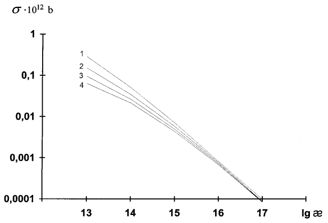
Figure 1: The cross section of the process $e+\gamma\to e+Z+H$ as a function of $\ae$ for various values of the Higgs mass: $M_{H}=100$ (1), 200 (2), 300 (3),    400 (4) GeV

$$\sigma(e^{+}+e^{-}\to Z+H)=\frac{G^{2}_{f}M^{4}_{Z}}{48\pi s}(1-4\sin^{2}\Theta_{W}+8\sin^{4}\Theta_{W}),$$ (18)

whereas with consideration for (6) the rate of the Higgs boson production channel $e+\gamma\to e+Z+H$ in the logarithmic approximation ($\ln\frac{\displaystyle\ae m^{2}}{\displaystyle M^{2}}\gg 1$) is described as

$$\sigma(e^{-}+\gamma\to e^{-}+Z+H)=\left\{\sigma_{1},\;k\gg 1,\atop\sigma_{2},\;k\ll 1,\right.$$

$$k=\frac{1}{\ae}\left(\frac{M_{Z}}{m}\right)^{4}\ln\frac{\ae m^{2}}{M^{2}},$$

$$\sigma_{1}=\frac{1}{3}(g_{V}-g_{A})^{2}\left(\frac{eG_{f}m}{\pi}\right)^{2}\frac{1}{\ae}\left(\frac{M_{Z}}{m}\right)^{4}\ln\left(\frac{\ae m}{M}\right)\ln\left(\frac{\ae m^{2}}{M^{2}}\right),$$ (19)

$$\sigma_{2}=\frac{2}{3}g^{2}_{A}\left(\frac{eG_{f}m}{\pi}\right)^{2}\ln\frac{\ae m^{2}}{M^{2}}.$$

The study of (18), (19) for the head-on electron–photon collisions when the energies of the particles are equal, leads to the following ratio of the cross sections:

$$\frac{\sigma(e+\gamma\to e+Z+H)}{\sigma(e^{+}+e^{-}\to Z+H)}\cong\left\{C_{1},\;k\gg 1,\,\,\ae\ll 10^{22},\atop C_{2},\;k\ll 1,\,\,\ae\gg 10^{23},\right.$$

$$C_{1}=5\alpha\ln\left(\frac{2E}{m}\right)\ln\left(\frac{4E^{2}}{Mm}\right),\;C_{2}=\alpha\ln\left(\frac{2E}{M}\right)\ae\left(\frac{m}{M_{Z}}\right)^{4},$$ (20)

where $\alpha$ is the fine structure constant.

The results obtained (19), (20) are valid in the wide range of external field intensities, and energy values. For example, if $E>1000$ GeV, the ratio of the cross sections of the processes compared is equal to $C_{1}>10.$

Thus, as it follows from (20), at least at high energies the cross section of the reaction examined can substantially exceed that of the process $e^{+}+e^{-}\to Z+H,$ which at present is considered to be the most probable channel for the Higgs boson production.

References

[1]
J.–F. Grivaz, Preprint LAL 97–60, 19 (1997).
[2]
L.B. Okun, Leptons and Quarks (Nauka, Moskow, 1989), in Russian.
[3]
V. Barger, K. Cheung, R. J. N. Phillips et al., Phys.Rev. D 46,
3725 (1992).
[4]
V. Barger, K. Cheung, A. Djouadi et al., Phys. Rev. D 49, 79 (1994).
[5]
E. Boos, M. Sachnitz, H. J. Schreiber et al., Int. J. Mod. Phys. A 10
2067 (1995).
[6]
W. Kilian, M. Kramer, P. M. Zervas, Phys. Lett. B 373, 135 (1996).
[7]
P. M. Zerwas, Preprint DESY 94-001, 46, Updated May 1996.
[8]
J. Kuti, Lee Lin Yue Shen, Phys. Rev. Lett. 61, 678 (1988).
[9]
G. Altrelli, G. Isidori, Phys. Lett. B 337, 141 (1994).
[10]
J. Casas, J. Espinosa, M. Quiros, Phys. Lett. B 342, 171 (1995).
[11]
K. Hagiroara, I. Watanabe, P. M. Zerwas, Phys. Lett. B 278, 187 (1992).
[12]
O. J. P. Eboli, M. C. Gonzales–Garsia, S. F. Novaes, Phys. Rev. D 49,
91 (1994).
[13]
I.M. Ternov, V.Ch. Zhukovskii and A.V. Borisov, Quantum
Processes in Strong External Field (Moscow State University, Moscow,
1989), in Russian.
[14]
V.I. Ritus, Fiz. Inst. Akad. Nauk SSSR 111, 5 (1979);
A.I. Nikishov, Fiz. Inst. Akad. Nauk SSSR 111, 152 (1979).