[

A Strong Electroweak Phase Transition up to $m_{H}\sim 105$ GeV

Abstract

Non-perturbative lattice simulations have shown that there is no electroweak phase transition in the Standard Model for the allowed Higgs masses, $m_{H}\mathop{\raise 1.29167pt\hbox{$>$\kern-7.5pt\raise-4.73611pt\hbox{$\sim$}}}75$ GeV. In the Minimal Supersymmetric Standard Model, in contrast, it has been proposed that the transition should exist and even be strong enough for baryogenesis up to $m_{H}\sim 105$ GeV, provided that the lightest stop mass is in the range 100…160 GeV. However, this prediction is based on perturbation theory, and suffers from a noticeable gauge parameter and renormalization scale dependence. We have performed large-scale lattice Monte Carlo simulations of the MSSM electroweak phase transition. Extrapolating the results to the infinite volume and continuum limits, we find that the transition is in fact stronger than indicated by 2-loop perturbation theory. This guarantees that the perturbative Higgs mass bound $m_{H}\sim 105$ GeV is a conservative one, allows slightly larger stop masses (up to $\sim$ 165 GeV), and provides a strong motivation for further studies of MSSM electroweak baryogenesis.

CERN-TH/98-121, NORDITA-98/28P, hep-ph/9804255

]

It is known from studies of primordial nucleosynthesis that there is a non-vanishing baryon to photon density ratio in the Universe, $\eta\approx 10^{-10}$ (for recent reviews, see [1]). It is one of the main challenges of cosmology to understand how such an asymmetry could come about. Indeed, different scenarios for producing $\eta>0$ abound.

Among all the scenarios for baryogenesis, one is unique: the last instance in the history of the Universe that a baryon asymmetry could have been generated, is the electroweak phase transition [2]. As such, this is also the scenario requiring the least assumptions beyond established physics. In principle, even the Standard Model contains the necessary ingredients for baryon number generation: anomalous baryon number violation, CP-violation, and an electroweak phase transition providing for a non-equilibrium environment (for a review, see [3]). Once an asymmetry has been generated, it must also be preserved, and this gives a strict constraint on how strongly of the first order the transition must be [2]. In fact, the constraint on the strength of the phase transition is the most rigorous of the constraints mentioned, since it concerns a thermodynamical equilibrium situation after the transition, and equilibrium physics is much better understood than non-equilibrium physics.

However, it turns out that on a more quantitative level the Standard Model is too restricted for baryogenesis. The main reason is that the strength of the electroweak phase transition depends on the Higgs mass, and for the allowed values $m_{H}\mathop{\raise 1.29167pt\hbox{$>$\kern-7.5pt\raise-4.73611pt\hbox{$\sim$}}}75$ GeV, there is no electroweak phase transition at all [4, 5]. The existence of the baryon asymmetry alone thus requires physics beyond what is currently known.

The simplest extended scenarios that allow for baryon asymmetry generation at the electroweak phase transition, have a Higgs sector which differs from that in the Standard Model. A particularly appealing scenario is the electroweak phase transition in the MSSM [6–8]. Indeed, it has recently become clear that the electroweak phase transition can then be much stronger than in the Standard Model, and strong enough for baryogenesis at least for Higgs masses up to 80 GeV [9–16]. For the lightest stop mass $m_{\tilde{t}_{R}}$ lighter than the top mass, one can go even up to $\sim$ 100 GeV [17]: in the most recent analysis [18], the allowed window was estimated at $m_{H}\sim 75\ldots 105$ GeV, $m_{\tilde{t}_{R}}\sim 100\ldots 160$ GeV. In this regime, the transition could even proceed in two stages [17], via an exotic intermediate colour breaking minimum. This Higgs and stop mass window is interesting from an experimental point of view, as well, as the whole range will be covered at LEP and the Tevatron [18].

Unfortunately, the statement concerning the strength of the electroweak phase transition in this regime is subject to large uncertainties. The first indication in this direction is that the 2-loop corrections to the Higgs field effective potential are large and strengthen the transition considerably [10]. A further sign is that the gauge parameter and, in particular, the renormalization scale dependence of the 2-loop potential, which are formally of the 3-loop order, are numerically quite significant [17]. Hence a non-perturbative analysis is needed.

The purpose of this paper is to study the MSSM electroweak phase transition with lattice Monte Carlo simulations, and to extrapolate the results to the infinite volume and continuum limits. Since the MSSM at finite temperature is a multiscale system with widely different scales from $\sim\pi T$ to $\sim g_{W}^{2}T$, and since there are chiral fermions, the only way to do the simulations in practice is to use an effective 3d theory [19]. This approach consists of a perturbative dimensional reduction into a 3d theory with considerably fewer degrees of freedom than in the original theory [21–23], and of lattice simulations in the effective theory. The analytical dimensional reduction step has been performed for the MSSM in [12–14,17]. Lattice simulations in dimensionally reduced 3d theories have been previously used to determine the properties of the electroweak phase transition in the Standard Model in great detail [24–30].

In the regime considered, the right-handed stop field $U$ plays an important role in addition to the Higgs field. The effective 3d Lagrangian describing the electroweak phase transition in the MSSM is therefore an SU(3)$\times$SU(2) gauge theory with two scalar fields [12, 17]:

$${\cal L}_{\rm cont}^{\rm 3d} = {\frac{1}{4}}F^{a}_{ij}F^{a}_{ij}+{\frac{1}{4}}G^{A}_{ij}G^{A}_{ij}+\gamma H^{\dagger}HU^{\dagger}U$$ (1)

$$+ (D_{i}^{w}H)^{\dagger}(D_{i}^{w}H)+(D_{i}^{s}U)^{\dagger}(D_{i}^{s}U)+m_{H3}^{2}H^{\dagger}H$$ (2)

$$+ m_{U3}^{2}U^{\dagger}U+\lambda_{H}(H^{\dagger}H)^{2}+\lambda_{U}(U^{\dagger}U)^{2}.$$ (3)

Here $D_{i}^{w}$ and $D_{i}^{s}$ are the SU(2) and SU(3) covariant derivatives, and $H$ is the combination of the Higgs doublets which is “light” at the phase transition point. The U(1) subgroup of the Standard Model induces only small perturbative contributions [30], and can be neglected.

The complexity of the original 4d Lagrangian is hidden in Eq. (3) in the expressions of the parameters of the 3d theory. A dimensional reduction computation leading to actual expressions for these parameters has been made in [17] for a particularly simple case. Let us stress here that the reduction is a purely perturbative computation and is free of infrared problems. The relative error has been estimated in [12, 17], and should be $\mathop{\raise 1.29167pt\hbox{$<$\kern-7.5pt\raise-4.73611pt\hbox{$\sim$}}}10\%$.

It is prohibitively time-consuming to study the full parameter space of Eq. (3) with Monte Carlo simulations. Thus, we only consider a special parameter choice: we take a large left-handed squark mass parameter $m_{Q}\sim$1 TeV, vanishing squark mixing parameters, and a heavy CP-odd Higgs particle ($m_{A}\mathop{\raise 1.29167pt\hbox{$>$\kern-7.5pt\raise-4.73611pt\hbox{$\sim$}}}300$ GeV). We fix $\tan\beta=3$, corresponding to $m_{H}\sim 95$ GeV. We then study the 3d theory in Eq. (3), parametrized by the temperature $T$ and the right-handed stop mass parameter $\tilde{m}_{U}$ ($\tilde{m}_{U}$ determines the zero temperature right-handed stop mass through $m_{\tilde{t}_{R}}\approx({m_{\rm top}^{2}-\tilde{m}_{U}^{2}})^{1/2}$). The actual expressions used for the dimensional reduction are given in [31].

The philosophy is now that we determine the non-perturbative results for the continuum theory in Eq. (3) through lattice simulations, and compare them with 3d perturbation theory, employing the same 3d parameters. To be more precise, we compare with 2-loop 3d perturbation theory in the Landau gauge $\xi=0$ and for the $\overline{\mbox{\rm MS}}$ scale parameter $\bar{\mu}=T$, values which have been used in [18], as well. This allows one to find out whether there are any non-perturbative effects in the system. Once this has been done, one can go back to a more complicated situation and study it perturbatively, adding to the perturbative results the non-perturbative effects found here. As the reduction step is purely perturbative, the non-perturbative effects found with the 3d approach apply also to the effective potential computed in 4d [10, 16, 18].

To perform lattice simulations, we discretize the theory in Eq. (3) with standard methods (see [31]). The lattice parameters are expressed in terms of the lattice spacing $a$ and the continuum parameters through 2-loop relations [32] which become exact in the continuum limit.

Well controlled infinite volume and continuum limits are essential in order to obtain reliable results. Thus, for each point in the parameter space, we always perform simulations with several lattice volumes and extrapolate to the infinite volume. We use the lattice spacings obtained through

$$\beta_{S}\equiv{\frac{6}{g_{S3}^{2}a}}=12,20,$$ (4)

where $g_{S3}^{2}=g_{S}^{2}T\sim T$ is the 3d SU(3) gauge coupling and $a$ is the lattice spacing. The fact that we use just two values of $\beta_{S}$, only allows a linear extrapolation to the continuum limit $\beta_{S}=\infty$. However, it is understood analytically that the dominant corrections are linear [33], and moreover, linear extrapolations work extremely well for the case of the Standard Model [25, 30].

All in all, we have performed 42 different Monte Carlo runs: combinations of lattice sizes and parameters. The total cpu-time was $\sim$7.5 node-years on a Cray T3E.

The physical quantities we discuss here are the critical temperature $T_{c}$, the scalar field expectation values, and the latent heat. Quantities such as the latent heat enter, for instance, the estimates for the nucleation and reheating temperatures (see, e.g., [34]), which are needed to decide whether the scalar field expectation values relevant for cosmology should be taken at $T_{c}$ or some lower temperature.

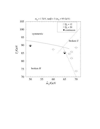
FIG. 1.: The phase diagram and the critical temperatures. The continuous lines are from the 2-loop perturbative effective potential in the Landau gauge. Open symbols correspond to infinite volume extrapolations, and filled symbols to continuum limit extrapolations.

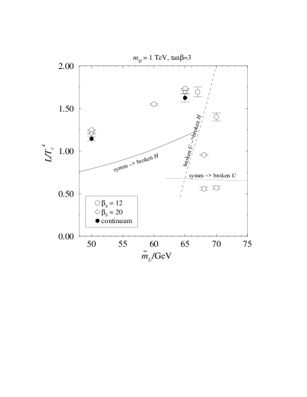
FIG. 2.: The latent heat.

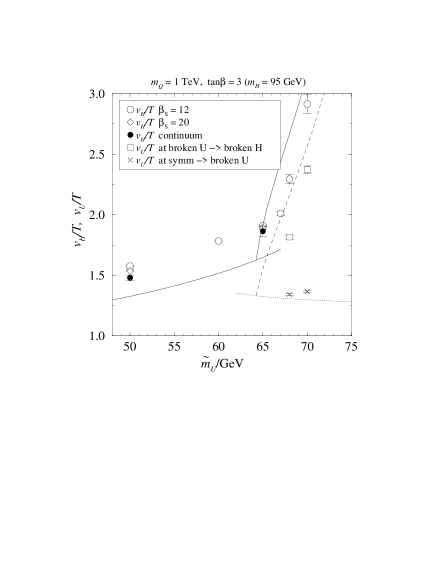
FIG. 3.: The scalar field expectation values in the broken phases at $T_{c}$.

1. The phase diagram and the critical temperatures.  
The general phase structure of the theory is expected to be the following [17]. The system has a first order transition at $T_{c}\sim 100$ GeV for $\tilde{m}_{U}\mathop{\raise 1.29167pt\hbox{$<$\kern-7.5pt\raise-4.73611pt\hbox{$\sim$}}}65$ GeV. This transition is strong even though $m_{H}$ is large, due to the stop loops. As $\tilde{m}_{U}$ becomes larger ($m_{\tilde{t}_{R}}$ smaller), the transition gets even stronger, and then at some point one may get a two-stage transition. The existence of a two-stage transition depends on the parameters of the theory, and for large squark mixing parameters the two-stage region is not reached [18].

Our numerical results are shown in Fig. 1. It is seen that the phase diagram is qualitatively the same as in perturbation theory, although the critical temperatures and the triple point have been displaced by a few GeV. We have data at $\beta_{S}=20$ only at $\tilde{m}_{U}=50$, 65 GeV, and the continuum extrapolation is possible only at these points. Nevertheless, we expect similar (small) effects at the other points. As of now, we have no clear theoretical explanation for the discrepancy between the lattice results and perturbation theory: the reason might be, e.g., a three-loop perturbative effect, or a genuine non-perturbative contribution.

2. Latent heat.  
The main result of this paper is shown in Fig. 2, which shows the latent heat. It is the most important gauge-invariant physical characterization of the strength of a first order transition. We observe that the non-perturbative transition to the standard electroweak minimum at $\tilde{m}_{U}\mathop{\raise 1.29167pt\hbox{$<$\kern-7.5pt\raise-4.73611pt\hbox{$\sim$}}}67$ GeV is significantly (up to 45%) stronger than the perturbative transition. In the regime $\tilde{m}_{U}\mathop{\raise 1.29167pt\hbox{$>$\kern-7.5pt\raise-4.73611pt\hbox{$\sim$}}}67$ GeV where there is a two-stage transition, a comparison with perturbation theory is more difficult as the whole pattern is shifted to the right, but the qualitative behaviour is the same.

3. Scalar field expectation values.  
The Higgs field vacuum expectation value $v_{H}$ is the object by which one usually characterises whether the phase transition is strong enough for baryogenesis [2, 3], the requirement being $v_{H}/T\mathop{\raise 1.29167pt\hbox{$>$\kern-7.5pt\raise-4.73611pt\hbox{$\sim$}}}1$. As such $v_{H}$ is, however, a gauge dependent quantity. If one computes it in the Landau gauge ($v_{H}^{L}$), as is usual, then in terms of gauge-invariant operators the same expression would be non-local. On the other hand, there is a simple local gauge-invariant quantity closely related to $v_{H}$, namely $H^{\dagger}H\sim v_{H}^{2}/2$. The problem with $H^{\dagger}H$ is that being a composite operator, it is a scale dependent quantity in, say, the $\overline{\mbox{\rm MS}}$ scheme. We hence define on the lattice

$$\frac{v_{H}}{T}\equiv\left(2\left\langle\frac{H^{\dagger}H_{\overline{\mbox{\rm MS}}}(g_{S3}^{2})}{T}\right\rangle\right)^{1/2},$$ (5)

which is a natural gauge-invariant generalization of $v_{H}^{L}/T$, and can be measured in simulations. Note that with respect to 4d units, there is a trivial rescaling by $T$ in the $H^{\dagger}H$ appearing in Eq. (5).

The numerical results for $v_{H}/T,v_{U}/T$ are shown in Fig. 3. Again, we observe a value larger than in perturbation theory in the regime $\tilde{m}_{U}\mathop{\raise 1.29167pt\hbox{$<$\kern-7.5pt\raise-4.73611pt\hbox{$\sim$}}}67$ GeV. Moreover, in qualitative accordance with perturbation theory, there is a rapid increase in $v_{H}/T_{c}$ in the regime of the two-stage transition, $\tilde{m}_{U}\mathop{\raise 1.29167pt\hbox{$>$\kern-7.5pt\raise-4.73611pt\hbox{$\sim$}}}67$ GeV. The relative non-perturbative strengthening effect is smaller than for the latent heat, which is easy to understand since $L\propto\Delta(H^{\dagger}H)\sim\Delta v_{H}^{2}$ [25], implying $\delta L/L\sim 2\delta v_{H}/v_{H}$.

In conclusion, at least for the parameter values studied ($m_{H}\sim 95$ GeV, $m_{\tilde{t}_{R}}\sim 150\ldots 160$ GeV), the electroweak phase transition is significantly stronger than indicated by 2-loop perturbation theory. This implies that the previous perturbative Higgs and stop mass bounds for electroweak baryogenesis are conservative estimates. In particular, the electroweak phase transition could be strong enough for baryogenesis for all allowed Higgs masses in this regime ($m_{H}\mathop{\raise 1.29167pt\hbox{$<$\kern-7.5pt\raise-4.73611pt\hbox{$\sim$}}}105$ GeV) [18]. Due to the non-perturbative strengthening effect seen, the stop mass could be slightly larger than the perturbative value, up to $m_{\tilde{t}_{R}}\sim 165$ GeV. For the smallest stop masses, on the other hand, there is the possibility of a two-stage transition, in which the Higgs field gets an extremely large vacuum expectation value.

These results provide a strong motivation for precise studies of the non-equilibrium CP-violating real time dynamics and baryon number generation at the MSSM electroweak phase transition.

Acknowledgements. The simulations were made with a Cray T3E at the Center for Scientific Computing, Finland. We acknowledge useful discussions with K. Kajantie, G.D. Moore, M. Shaposhnikov and C. Wagner. This work was partly supported by the TMR network Finite Temperature Phase Transitions in Particle Physics, EU contract no. FMRX-CT97-0122.

REFERENCES

- [1] K.A. Olive, talk given at 5th International Workshop on Topics in Astroparticle and Underground Physics (TAUP 97), Gran Sasso, Italy, 7-11 Sep 1997 [astro-ph/9712160]; G. Steigman, talk given at 2nd Oak Ridge Symposium on Atomic and Nuclear Astrophysics, Oak Ridge, 2-6 Dec 1997 [astro-ph/9803055].
- [2] V.A. Kuzmin, V.A. Rubakov and M.E. Shaposhnikov, Phys. Lett. B 155, 36 (1985); M.E. Shaposhnikov, Nucl. Phys. B 287, 757 (1987).
- [3] V.A. Rubakov and M.E. Shaposhnikov, Usp. Fiz. Nauk 166, 493 (1996) [hep-ph/9603208].
- [4] K. Kajantie, M. Laine, K. Rummukainen and M. Shaposhnikov, Phys. Rev. Lett. 77, 2887 (1996).
- [5] M. Gürtler, E.-M. Ilgenfritz and A. Schiller, Phys. Rev. D 56, 3888 (1997).
- [6] S. Myint, Phys. Lett. B 287, 325 (1992); G.F. Giudice, Phys. Rev. D 45, 3177 (1992).
- [7] J.R. Espinosa, M. Quirós and F. Zwirner, Phys. Lett. B 307, 106 (1993).
- [8] A. Brignole, J.R. Espinosa, M. Quirós and F. Zwirner, Phys. Lett. B 324, 181 (1994).
- [9] M. Carena, M. Quirós and C.E.M. Wagner, Phys. Lett. B 380, 81 (1996).
- [10] J.R. Espinosa, Nucl. Phys. B 475, 273 (1996).
- [11] D. Delepine, J.-M. Gérard, R. Gonzalez Felipe and J. Weyers, Phys. Lett. B 386, 183 (1996).
- [12] M. Laine, Nucl. Phys. B 481, 43 (1996).
- [13] J.M. Cline and K. Kainulainen, Nucl. Phys. B 482, 73 (1996); Nucl. Phys. B 510, 88 (1998).
- [14] M. Losada, Phys. Rev. D 56, 2893 (1997); G.R. Farrar and M. Losada, Phys. Lett. B 406, 60 (1997).
- [15] J.M. Moreno, D.H. Oaknin and M. Quirós, Nucl. Phys. B 483, 267 (1997); Phys. Lett. B 395, 234 (1997).
- [16] B. de Carlos and J.R. Espinosa, Nucl. Phys. B 503, 24 (1997).
- [17] D. Bödeker, P. John, M. Laine and M.G. Schmidt, Nucl. Phys. B 497, 387 (1997).
- [18] M. Carena, M. Quirós and C.E.M. Wagner, CERN-TH/97-190 [hep-ph/9710401].
- [19] 4d lattice simulations have been performed for the Standard Electroweak Model without fermions [20]. However, the simulations are extremely demanding: even with an unrealistically large gauge coupling and without an extrapolation to the continuum limit, the relative error on quantities such as the latent heat was more than 40%.
- [20] F. Csikor, Z. Fodor, J. Hein, A. Jaster and I. Montvay, Nucl. Phys. B 474, 421 (1996), and references therein; Y. Aoki, Phys. Rev. D 56, 3860 (1997).
- [21] P. Ginsparg, Nucl. Phys. B 170, 388 (1980); T. Appelquist and R. Pisarski, Phys. Rev. D 23, 2305 (1981).
- [22] K. Farakos, K. Kajantie, K. Rummukainen and M. Shaposhnikov, Nucl. Phys. B 425, 67 (1994); K. Kajantie, M. Laine, K. Rummukainen and M. Shaposhnikov, Nucl. Phys. B 458, 90 (1996).
- [23] A. Jakovác and A. Patkós, Phys. Lett. B 334, 391 (1994); Nucl. Phys. B 494, 54 (1997); E. Braaten and A. Nieto, Phys. Rev. D 51, 6990 (1995); Phys. Rev. D 53, 3421 (1996).
- [24] K. Kajantie, K. Rummukainen and M. Shaposhnikov, Nucl. Phys. B 407, 356 (1993).
- [25] K. Kajantie, M. Laine, K. Rummukainen and M. Shaposhnikov, Nucl. Phys. B 466, 189 (1996).
- [26] E.-M. Ilgenfritz, J. Kripfganz, H. Perlt and A. Schiller, Phys. Lett. B 356, 561 (1995); M. Gürtler, E.-M. Ilgenfritz, J. Kripfganz, H. Perlt and A. Schiller, Nucl. Phys. B 483, 383 (1997); M. Gürtler, E.-M. Ilgenfritz and A. Schiller, Eur. Phys. J. C 1, 363 (1998).
- [27] F. Karsch, T. Neuhaus, A. Patkós and J. Rank, Nucl. Phys. B 474, 217 (1996).
- [28] O. Philipsen, M. Teper and H. Wittig, Nucl. Phys. B 469, 445 (1996); OUTP-97-44-P [hep-lat/9709145].
- [29] G.D. Moore and N. Turok, Phys. Rev. D 55, 6538 (1997).
- [30] K. Kajantie, M. Laine, K. Rummukainen and M. Shaposhnikov, Nucl. Phys. B 493, 413 (1997).
- [31] M. Laine and K. Rummukainen, CERN-TH/98-122, to appear.
- [32] M. Laine and A. Rajantie, Nucl. Phys. B 513, 471 (1998).
- [33] G.D. Moore, McGill-97-23 [hep-lat/9709053].
- [34] H. Kurki-Suonio and M. Laine, Phys. Rev. Lett. 77, 3951 (1996).